The University of Adelaide
School of Economics
Research Paper No. 2009-01
January 2009
Bandwidth Selection in Nonparametric
Kernel Testing
Bandwidth Selection in Nonparametric Kernel Testing
1 By Jiti Gao and Ir`ene GijbelsThe University of Adelaide and Katholieke Universiteit Leuven
Abstract. We propose a sound approach to bandwidth selection in nonparametric ker-nel testing. The main idea is to find an Edgeworth expansion of the asymptotic distribution of the test concerned. Due to the involvement of a kernel bandwidth in the leading term of the Edgeworth expansion, we are able to establish closed–form expressions to explicitly represent the leading terms of both the size and power functions and then determine how the bandwidth should be chosen according to certain requirements for both the size and power functions. For example, when a significance level is given, we can choose the band-width such that the power function is maximized while the size function is controlled by the significance level. Both asymptotic theory and methodology are established. In addition, we develop an easy implementation procedure for the practical realization of the established methodology and illustrate this on two simulated examples and a real data example.
Keywords: Choice of bandwidth parameter, Edgeworth expansion, nonparametric ker-nel testing, power function, size function.
1Jiti Gao is Professor of Economics, School of Economics, The University of Adelaide, Adelaide
SA 5005, Australia (E–mail: [email protected]). Irene Gijbels is Professor of Statistics, De-partment of Mathematics, University of Leuven, Celestijnenlaan 200B, B-3001, Leuven, Belgium (E–mail: [email protected]). The first author would like to thank Jiying Yin for his excellent computing assistance and the Australian Research Council Discovery Grants under Grant Numbers: DP0558602 and DP0879088 for the financial support. The second author thanks the School of Mathematics and Statistics at the University of Western Australia for its kind hospital-ity and support. The second author also gratefully acknowledges the Research Fund K.U.Leuven (GOA/2007/4) and the Flemish Science Foundation, FWO Belgium (Project G.0328.08) for financial support.
1. Introduction
Consider a nonparametric regression model of the form
Yi =m(Xi) +ei, i= 1,2, . . . , n, (1.1)
where{Xi}is a sequence of strictly stationary time series variables,{ei}is a sequence
of independent and identically distributed (i.i.d.) errors with E[e1] = 0 and 0 <
E[e2
1] = σ2 < ∞, m(·) is an unknown function defined over IRd for d ≥ 1, and n is
the number of observations. We assume that {Xi} and {ej} are independent for all
1≤i≤j ≤n.
To avoid the so–called “curse of dimensionality” problem, we mainly consider
the case of 1 ≤ d ≤ 3 in this paper. For the case of d ≥ 4, various dimension
reduction estimation and specification methods have been discussed extensively in several monographs, such as Fan and Gijbels (1996), Hart (1997), Fan and Yao (2003), Gao (2007), and Li and Racine (2007).
There is a vast literature on testing a parametric regression model (null hypoth-esis) versus a nonparametric model, especially for the case of i.i.d. Xi’s (random or
fixed design case). Many goodness-of-fit testing procedures are based on evaluating a distance between a parametric estimate of the regression functionm (assuming the null hypothesis is true) and a nonparametric estimate of that function. Among the popular choices for a nonparametric kernel estimator formare the Nadaraya-Watson estimator, the Gasser-M¨uller estimator and a local linear (polynomial) estimator. Earlier papers following this approach of evaluating such a distance include H¨ardle and Mammen (1993), Weihrather (1993) and Gonz´alez-Manteiga and Cao (1993), among others. H¨ardle and Mammen (1993) consider a weightedL2-distance between
a parametric estimator and a nonparametric Nadaraya-Watson estimator of the re-gression function. The asymptotic distribution of their test statistic under the null hypothesis depends on the unknown error variance (the conditional error variance function). Weihrather (1993) instead uses a Gasser-M¨uller nonparametric estimator
in the fixed design regression case, divides by an estimator of the error variance and considers a discretized version of theL2-distance. Gonz´alez-Manteiga and Cao (1993)
also consider the fixed design regression case but rely on minimum distance estimation of the parametric model, seeking for minimizing a weightedL2-type distance between
the parametric model and a pilot nonparametric estimator.
Another approach to the same testing problem is introduced in Dette (1999) who focusses on the integrated conditional variance function, and uses as a test statis-tic the difference of a parametric estimator and a nonparametric (Nadaraya-Watson based) estimator of this integrated variance. It is shown that this estimator (asymp-totically) corresponds to test statistics based on a weighted L2-distance between a
parametric and nonparametric estimator of the regression function, as in the above mentioned papers, using an appropriate weight function in defining theL2-distance.
Dette (1999) studies the asymptotic distribution of the test statistic under fixed alter-natives. Such kind of alternatives are to be distinguished from the so-called sequences of local alternatives, where the difference between the regression function under the alternative and the one under the null hypothesis depends on the sample size n and decreases with n. The latter setup is the one considered in our study.
The above papers and several more recent goodness-of-fit tests (see for example Zhang and Dette (2004) and references therein) have in common that they rely on nonparametric kernel type regression estimators and that the resulting test statis-tics are of a similar form (at least in first-order asymptostatis-tics), and all depend on a bandwidth parameter. The choice of the bandwidth parameter in such goodness-of-fit testing procedures is the main concern in the present paper. Roughly speaking one can distinguish in the literature two approaches to deal with this bandwidth parame-ter choice in nonparametric and semiparametric kernel methods used for constructing model specification tests for the mean function of model (1.1). A first approach is to use an estimation-based optimal bandwidth value, such as a cross–validation band-width. A second approach is to consider a set of suitable values for the bandwidth
and proceed further from there.
Existing studies based on the first approach include H¨ardle and Mammen (1993) for testing nonparametric regression with i.i.d. designs and errors, Hjellvik and Tjøstheim (1995), and Hjellvik, Yao and Tjøstheim (1998) for testing linearity in dependent time series cases, Li (1999) for specification testing in econometric time series cases, Chen, H¨ardle and Li (2003) for using empirical likelihood–based tests, Juhl and Xiao (2005) for testing structural change in nonparametric time series re-gression, and others. As pointed out in the literature, such choices cannot be justified in both theory and practice since estimation–based optimal values may not be optimal for testing purposes.
Nonparametric tests involving the second approach of choising either a set of suitable bandwidth values for the kernel case or a sequence of positive integers for the smoothing spline case include Fan (1996), Fan, Zhang and Zhang (2001), and Horowitz and Spokoiny (2001). The practical implementation of choosing such sets or sequences is however problematic. This is probably why Horowitz and Spokoiny (2001) develop their theoretical results based on a set of suitable bandwidths on the one hand, but choose their practical bandwidth values based on the assessment of the power function of their test on the other hand. Apart from using such test statistics based on nonparametric kernel, nonparametric series, spline smoothing and wavelet methods, there are test statistics constructed and studied based on empirical distributions. Such studies have recently been summarized in Zhu (2005).
To the best of our knowledge, the idea of choosing the appropriate smoothing parameter such that the size of the test under consideration is preserved while max-imizing the power against a given alternative was only first explored analytically by Kulasekera and Wang (1997), in which the authors propose using a nonparametric kernel test to check whether the mean functions of two data sets can be identical in a nonparametric fixed design setting. In some other closely related studies, various discussions have been given on the comparison of power values of the same test at
different bandwidths or different tests at the same bandwidth. Such studies include Hart (1997), Hjellvik, Yao and Tjøstheim (1998), Hunsberger and Follmann (2001), and Zhang and Dette (2004). The last paper compares three main types of nonpara-metric kernel tests proposed in H¨ardle and Mammen (1993), Zheng (1996), and Fan, Zhang and Zhang (2001).
On the issue of size correction, there have recently been some studies. For example, Fan and Linton (2003) develop an Edgeworth expansion for the size function of their test and then propose using corrected asymptotic critical values to improve the small– medium sample size properties of the size of their test. Some other related studies include Nishiyama and Robinson (2000), Horowitz (2003), Nishiyama and Robinson (2005), who develop some useful Edgeworth expansions for bootstrap distributions of partial–sum type of tests for improving the size performance.
The current paper is motivated by such existing studies, especially by Kulasek-era and Wang (1997), Fan and Linton (2003), Dette and Spreckelsen (2004), and Zhang and Dette (2004), to develop a solid theory to support a power function–based bandwidth selection procedure such that the power of the proposed test is maximized while the size is under control when using nonparametric kernel testing in parametric specification of a nonparametric regression model of the form (1.1) associated with the hypothesis form of (1.2) below.
To state the main results of this paper, we introduce some notational details. The main interest of this paper is to test a parametric null hypothesis of the form
H0 : m(x) = mθ0(x) versus a sequence of alternatives of the form
H1 : m(x) = mθ1(x) + ∆n(x) for all x∈IR
d, (1.2)
where both θ0, θ1 ∈ Θ are unknown parameters and Θ is a parameter space of IRp,
and ∆n(x) is a sequence of nonparametrically unknown functions over IRd. With
∆n(x) not being equal to zero, the functionmθ1(x) in H1 is in fact the projection of
Note that m(x) under H1 in (1.2) is semiparametric when {∆n(x)} is unknown
nonparametrically. Note also that instead of requiring (1.2) for allx∈IRd, it may be
assumed that (1.2) holds with probability one forx=Xi. Some first–order asymptotic
properties for both the size and power functions of a nonparametric kernel test for the case where ∆n(·)≡∆(·), corresponding to a class of fixed alternatives (not depending
on n), have already been discussed in the literature, such as Dette and Spreckelsen (2004). This paper focuses on studying higher–order asymptotic properties of such kernel tests for the case where{∆n(·)}is a sequence of local alternatives in the sense
that limn→∞∆n(x) = 0 for all x∈IRd.
Let K(·) be the probability kernel density function and h be the bandwidth in-volved in the construction of a nonparametric kernel test statistic denoted byT!n(h).
To implement the kernel test in practice, we propose a new bootstrap simulation procedure to approximate the 1−α quantile of the distribution of the kernel test by a bootstrap simulated critical value lα. Let αn(h) = P
" ! Tn(h)> lα|H0 # and βn(h) = P " ! Tn(h)> lα|H1 #
be the respective size and power functions. In Theo-rem 2.2 we show that
αn(h) = 1−Φ(lα−sn)−κn (1−(lα−sn)2) φ(lα−sn) +o "√ hd#, (1.3) βn(h) = 1−Φ(lα−rn)−κn (1−(lα−rn)2) φ(lα−rn) +o "√ hd#, (1.4) where sn = p1 √ hd, r n = p2 n δn2 √ hd, κ n = p3 √
hd, and Φ(·) and φ(·) denote
respectively the cumulative distribution and density function of the standard Normal random variable, in which all pi’s are positive constants and δ2n =
$
∆2
n(x)π2(x)dx
with π(·) being the marginal density function of {Xi}.
Our aim is to choose a bandwidth hew such that βn(hew) = maxh∈Hn(α)βn(h)
with Hn(α) = {h : α−cmin < αn(h) < α+cmin} for some small 0 < cmin < α.
Our detailed study in Section 3 shows that hew is proportional to (n δn2)
−3
2d. Such
established relationship between δn and hew shows us that the choice of an optimal
Ifδnis chosen proportional ton−
d+12
6(d+4) for a sequence of local alternatives underH 1,
then the optimal rate ofhew is proportional ton− 1
d+4, which is the order of a
nonpara-metric cross–validation estimation–based bandwidth frequently used for testing pur-poses. When considering a sequence of local alternatives withδn =O
"
n−12√loglogn #
being chosen as the optimal rate for testing in this kind of kernel testing (Horowitz and Spokoiny 2001), the optimal rate of hew is proportional to (loglogn)−
3 2d.
The rest of the paper is organised as follows. Section 2 points out that existing nonparametric kernel tests can be decomposed with quadratic forms of{ei}as leading
terms in the decomposition. This motivates the discussion about establishing Edge-worth expansions for such quadratic forms. In Section 3, we apply the EdgeEdge-worth expansions to study both the size and power functions of a representative kernel test. Section 4 presents several examples of implementation. Some concluding remarks are made in Section 5. Mathematical assumptions and proofs are provided in the appendix.
2. Nonparametric kernel testing
As mentioned in the introductory section, various authors have discussed and studied nonparametric kernel test statistics based on a (weighted) L2–distance
func-tion between a nonparametric kernel estimator and a parametric counterpart of the mean function. It can be shown that the leading term of each of these nonparametric kernel test statistics is of a quadratic form (see, for example, Chen, H¨ardle and Li 2003) Pn(h) = n % i=1 n % j=1 ei w(Xi)Lh(Xi −Xj)w(Xj) ej, (2.1) where Lh(·) = n√1hdL " · h #
, L(x) = $ K(y)K(x+y)dy, and w(·) is a suitable weight function probably depending on either π(·), σ2(·) or both, in which K(·) is a
prob-ability kernel function, h is a bandwidth parameter and both are involved in a non-parametric kernel estimation ofm(·) .
In this paper, we concentrate on a second group of nonparametric kernel test statistics using a different distance function. Rewrite model (1.1) into a notational version of the form under H0
Y =mθ0(X) +e, (2.2)
whereX is assumed to be random and θ0 is the true value of θ underH0. Obviously,
E[e|X] = 0 underH0. Existing studies (Zheng 1996; Li and Wang 1998; Li 1999; Fan
and Linton 2003; Dette and Spreckelsen 2004; Juhl and Xiao 2005) propose using a distance function of the form
E[eE(e|X)π(X)] = E&"E2(e|X)#π(X)', (2.3) where π(·) is the marginal density function of X.
This suggests using a normalized kernel–based sample analogue of (2.3) of the form Tn(h) = 1 n√hd σ n n % i=1 n % j=1,&=i ei K (X i−Xj h ) ej, (2.4) whereσ2
n= 2µ22 ν2$ K2(u)duwith µk =E[ek1] for k ≥1 andνl =E[πl(X1)] for l≥1.
It can easily be seen thatTn(h) is the leading term of the following quadratic form
Qn(h) = 1 n√hd σ n n % i=1 n % j=1 ei K (X i −Xj h ) ej. (2.5)
In summary, both equations (2.1) and (2.5) can be generally written as
Rn(h) = n % i=1 n % j=1 ei φn(Xi, Xj)ej, (2.6)
where φn(·,·) may depend on n, the bandwidthh and the kernel function K.
Thus, it is of general interest to study asymptotic distributions and their Edge-worth expansions for quadratic forms of type (2.6). To present the main ideas of establishing Edgeworth expansions for such quadratic forms, we focus onTn(h) in the
expansion for the asymptotic distribution of each of such tests is the same as that for
Tn(h).
Since Tn(h) involves some unknown quantities, we estimate it by a stochastically
normalized version of the form
! Tn(h) = *n i=1 *n j=1,&=ie!i K "Xi−X j h # ! ej n√hd σ! n , (2.7)
where e!i = Yi − m!θ(Xi) and σ!n2 = 2µ!22 ν!2$ K2(u)du with µ!2 = n1 *ni=1e!2i and
!
ν2 = n1 *ni=1π!2(Xi), in which θ! is a √n–consistent estimator of θ0 under H0 and
! π(x) = 1 n!bd cv *n i=1K ( x−Xi !bcv )
is the conventional nonparametric kernel density estima-tor with!bcv being a bandwidth parameter chosen by cross–validation (see for example
Silverman 1986).
Similarly to existing results (Li 1999), it may be shown that for each given h
!
Tn(h) = Tn(h) +oP
"√
hd#. (2.8)
Thus, we may use the distribution of T!n(h) to approximate that of Tn(h). Let leα
(0 < α < 1) be the 1−α quantile of the exact finite–sample distribution of T!n(h).
Because le
α may not be evaluated in practice, we therefore suggest choosing either
a non–random approximate α–level critical value, lα, or a stochastic approximate
α–level critical value, l∗
α by using the following simulation procedure:
• We generateYi∗ =m!θ(Xi) +√µ!2 e∗i for 1≤i≤n, where {e∗i} is a sequence of
i.i.d. random samples drawn from a pre-specified distribution, such as N(0,1). Use the data set {(Xi, Yi∗) : i = 1,2, . . . , n} to estimate θ! by θ!∗ and compute
!
Tn(h). Let lα be the 1−α quantile of the distribution of
! Tn∗(h) = *n i=1 *n j=1,&=ie!∗i K "Xi−X j h # ! e∗ j n√hd σ!∗ n , (2.9) wheree!∗ i =Yi∗−m!θ∗(Xi) and σ!∗n2 = 2µ!∗22 ν!2$ K2(u)du with µ!∗2 = 1n *n i=1e!∗i2.
In the simulation process, the original sample Xn = (X1,· · ·, Xn) acts in the
• Repeat the above step M times and produce M versions of T!n∗(h) denoted by T!∗
n,m(h) for m = 1,2, . . . , M. Use the M values of T!n,m∗ (h) to construct
their empirical distribution function. The bootstrap distribution ofT!n∗(h) given
Wn ={(Xi, Yi) : 1≤i≤n}is defined byP∗ " ! Tn∗(h)≤x#=P"T!n∗(h)≤x|Wn # . Letl∗ α (0< α <1) satisfy P∗ " ! T∗ n(h)≥l∗α #
=α and then estimatelα byl∗α.
Note that both lα =lα(h) and l∗α =l∗α(h) depend on h. It should be pointed out
that the choice of a pre–specified distribution does not have much impact on both the theoretical and practical results. In addition, we may also use a wild bootstrap procedure to generate a sequence of resamples for{e∗
i}.
Note also that the above simulation is based on the so–called regression bootstrap simulation procedure discussed in the literature, such as Li and Wang (1998), Franke,
Kreiss and Mammen (2002), and Li and Racine (2007). When Xi = Yi−1, we may
also use a recursive simulation procedure, commonly-used in the literature. See for example, Hjellvik and Tjøstheim (1995), and Franke, Kreiss and Mammen (2002).
Since the choice of a simulation procedure does not affect the establishment of our theory, our main results are established based on the proposed simulation procedure. We now have the following results in Theorems 2.1 and 2.2; their proofs are provided in the appendix.
Theorem 2.1. Suppose that Assumptions A.1 and A.2 listed in the appendix hold. Then under H0 sup x∈R1 + + +P∗(T!n∗(h)≤x)−P(T!n(h)≤x) + + +=O"√hd# (2.10)
holds in probability with respect to the joint distribution of Wn, and
P"T!n(h)> l∗α
#
=α+O"√hd#. (2.11)
For an equivalent test, Li and Wang (1998) establish some results weaker than (2.10). Fan and Linton (2003) consider some higher–order approximations to the size function of the test discussed in Li and Wang (1998).
For each h we define the following size and power functions αn(h) = P " ! Tn(h)> lα|H0 # and βn(h) =P " ! Tn(h)> lα|H1 # . (2.12)
Correspondingly, we define (α∗n(h), βn∗(h)) withlα replaced by lα∗.
Before we discuss how to choose an optimal bandwidth in Section 3, we give Edgeworth expansions of both the size and power functions in Theorem 2.2 below. In order to express the Edgeworth expansions, we need to introduce the following notation. Let κn = √ hd"µ23K2(0) nhd + 4µ3 2ν3 3 K (3)(0)# σ3 n , (2.13)
where νl = E[πl(X1)] = $ πl+1(x)dx, and K(3)(·) is the three–time convolution of
K(·) with itself.
Theorem 2.2. (i) Suppose that Assumptions A.1 and A.2 listed in the appendix hold. Then αn(h) = 1−Φ(lα−sn)−κn (1−(lα−sn)2) φ(lα−sn) +o "√ hd#, (2.14) α∗n(h) = 1−Φ(lα∗ −sn)−κn (1−(l∗α−sn)2) φ(l∗α−sn) +o "√ hd# (2.15)
hold in probability with respect to the joint distribution of Wn, where Φ(·) and φ(·)
are the probability distribution and density functions of N(0,1), respectively, and
sn =C0(m) √ hd with C0(m) = $ "∂mθ0(x) ∂θ #τ( E,"mθ0(X1) ∂θ # "mθ 0(X1) ∂θ #τ-)−1"mθ 0(x) ∂θ # π2(x)dx . 2ν2 $ K2(v)dv .
(ii) Suppose that Assumptions A.1–A.3 listed in the appendix hold. Then the following equations hold in probability with respect to the joint distribution of Wn:
βn(h) = 1−Φ(lα−rn)−κn (1−(lα−rn)2) φ(lα−rn) +o "√ hd#, (2.16) βn∗(h) = 1−Φ(lα∗ −rn)−κn (1−(lα∗ −rn)2) φ(l∗α−rn) +o "√ hd#, (2.17)
where rn =n Cn2 √ hd, in which Cn2 = $ ∆2 n(x)π2(x)dx σ2.2ν 2 $ K2(v)dv . (2.18)
Assumption A.2 implies that the random quantity C0(m) is bounded in
probabil-ity. As expected, the rate of rn depends on the form of ∆n(·).
To simplify the following expressions, letzα be the 1−α quantile of the standard
normal distribution and dj = (zα2 −1)cj for j = 1,2, where
c1 = 4K(3)(0)µ32ν3 3σ3 n and c2 = µ23K2(0) σ3 n . (2.19)
Letd0 =d1−C0(m). A corollary of Theorem 2.2 is given in Theorem 2.3 below. Theorem 2.3. Suppose that the conditions of Theorem 2.2(i) hold. Then under
H0 lα ≈ zα+d0 √ hd+d 2 1 n√hd in probability, (2.20) lα∗ ≈ zα+d0 √ hd+d 2 1 n√hd in probability. (2.21)
Theorem 2.3 shows that the size distortion of the proposed test isd0
√
hd+d
2 n√1hd
when using the standard asymptotic normality in practice. A similar result has been obtained by Fan and Linton (2003). We show in addition that the bootstrap simulated critical value is approximated explicitly by zα+d0
√
hd+d
2 n√1hd.
As the main objective of this paper, Section 3 below proposes a suitable selection criterion for the choice of h such that while the size function is appropriately con-trolled, the power function is maximized at such h. A closed–form expression of the power function–based optimal bandwidth is given.
We now employ the Edgeworth expansions established in Section 2 to choose a suitable bandwidth such that the power function βn(h) is maximized while the size
function αn(h) is controlled by a significance level. We thus define
hew = arg max
h∈Hn(α)βn(h) with Hn(α) ={h: α−cmin < αn(h)< α+cmin} (3.1)
for some arbitrarily small cmin>0.
We now start to discuss how to solve the optimization problem (3.1). It follows from (2.13) and (2.19) that
κn= √ hd"µ23K2(0) nhd + 4µ3 2ν3 3 K(3)(0) # σ3 n =c1 √ hd+c 2 1 n√hd. (3.2) Let x=√hd. We rewriteκ n as κn=c1 x+c2 n−1 x−1. Let γn = (zα2 −1)κn, lα−rn ≈ zα+γn−rn=zα+ " d1−n Cn2 # x+d4 x−1≡zα+d3 x+d4 x−1, (3.3) lα−sn ≈ zα+γn−sn≈zα+ (d1−C0(m))x+d4 x−1 =zα+d0 x+d4 x−1,(3.4) where d0 = d1−C0(m), d1 = (zα2 −1)c1, d3 = d1−n Cn2 and d4 =c2 (z2α−1) n−1.
Note that limn→∞d4 = 0. Since Assumption A.3 implies that limn→∞n Cn2 = +∞,
we thus have
lim
n→∞d3 =−∞ when nlim→∞n C 2
n= +∞. (3.5)
Due to this, we treatd3 as a sufficiently large negative value whenn Cn2 is viewed
as a sufficiently large positive value in the finite–sample analysis of this section. Ignoring the higher–order terms (i.e. terms of order o(x+n−1x−1) or smaller),
we now re–write the power and size functions βn(h) andαn(h) simply as functions of
x=√hd as follows: βn(h) ≈ 1−Φ(lα−rn)−κn (1−(lα−rn)2) φ(lα−rn) ≈ 1−Φ(zα+d3x+d4x−1)− " c1x+c2n−1x−1 # × "1−(zα+d3x+d4x−1)2 # φ"zα+d3x+d4x−1 # ≡β(x), (3.6) αn(h) ≈ 1−Φ(lα−sn)−κn (1−(lα−sn)2) φ(lα−sn)
≈ 1−Φ(zα+d0x+d4x−1)− " c1x+c2n−1x−1 # × "1−(zα+d0x+d4x−1)2 # φ"zα+d0x+d4x−1 # ≡α(x). (3.7) Our objective is then to find xew=
.
hd
ew such that
xew = arg max
x∈Hn(α)β(x) with Hn(α) ={x: α−cmin < α(x)< α+cmin}, (3.8)
wherecmin is chosen ascmin = 10α for example. Finding roots ofβ((x) = 0 implies that
the leading order of the unique real root of the equation is given approximately by
hew =x 2 d ew =a− 1 2d 1 t −3 2d n , (3.9) wheretn=n Cn2,a1 = √ 2K(3)(0) 3".$K2(u)du# 3 ·c(π) with c(π) = $ π3(x)dx ".$ π2(x)dx# 3, in whichCn2 is
as defined in Theorem 2.2(ii).
It can also be shown that hew is the maximizer of the power function βn(h) at
h=hew such that
βn(((x)|x=√hd
ew <0, (3.10)
at least for sufficiently large n. Detailed derivations of (3.9) and (3.10) are given in Appendix B below.
Furthermore, the choice of hew satisfies both Assumptions A.1(v) and A.3 that
lim n→∞n h d ew = +∞ and nlim→∞n . hd ew Cn2 = +∞.
This implies that the choice of hew is valid to ensure limn→∞βn(hew) = 1.
When both σ2 = µ
2 = E[e21] and the marginal density function π(·) of {Xi} are
unknown in practice, we propose using an estimated version ofhew as follows:
! hew =!a− 1 2d 1 t! −3 2d n , (3.11) where ! tn = n C!n2 with C!n2 = 1 n *n i=1∆!2n(Xi)π!(Xi) ! µ2 . 2ν!2 $ K2(v)dv and ! a1 = √ 2K(3)(0) 3".$K2(u)du#3 ! c(π) with c!(π) = 1 n *n i=1π!2(Xi) ". 1 n *n i=1π!(Xi) #3,
in which µ!2, ν!2 and π!(·) are as defined in (2.7), and ∆!n(x) is given by ! ∆n(x) = *n i=1K ( x−Xi !bcv ) " Yi−m!θ(Xi) # *n i=1K ( x−Xi !bcv )
with θ!and !bcv being the same as in (2.7).
Note also that !hew provides an optimal bandwidth irrespectively of whether one
works under the null hypothesisH0 or under the alternative hypothesisH1. In other
words, it can be used for computing not only the power under an alternative H1,
but also the size under H0 in each case. Detailed discussion about this is given in
Appendix B below.
We conclude this section by summarizing the above discussion into the following proposition; its proof is given in Appendix B below.
Proposition 3.1. Suppose that Assumptions A.1–A.3 listed in the appendix hold. Additionally, suppose that ∆n(x) is continuously differentiable such that
lim
n→∞xsup∈Dπ
||∆(n(x)||
|∆n(x)| ≤
C <∞ and limn→∞infx∈IRd|∆n(x)|
.
n!bd
cv =∞ in probability
for some C > 0, where Dπ = {x ∈ IRd : π(x) > 0} and || · ||2 denotes the Euclidean
norm. Then lim n→∞ βn(h!ew) βn(hew) = 1 in probability. (3.12)
As pointed out in the introduction, implementation of each of existing nonpara-metric kernel tests involves either a single bandwidth chosen optimally for estimation purposes or a set of bandwidth values. The proposed !hew is chosen optimally for
testing purposes. Section 4 below shows how to implement the proposed test based on our bandwidth in practice and compares the finite–sample performance of the proposed choice with that of some closely relevant alternatives in the literature.
This section presents two simulated examples and one real data example to il-lustrate the proposed theory and methods in Sections 2 and 3 as well as to make comparisons with some closely relevant alternatives in the literature. Simulated ex-ample 4.1 below discusses the finite–sex-ample performance of the proposed testT!n(h!ew)
with that of the alternative version where the test is coupled with a cross–validation (CV) bandwidth choice. Simulated example 4.2 below compares our test with some of the commonly used tests in the literature. Example 4.3 provides a real data example to show that the proposed test makes a clear difference. In the following finite–sample study in Examples 4.1–4.3 below, we consider the case where ∆n(x) = cn ∆(x), in
which {cn}is a sequence of positive real numbers satisfying limn→∞cn = 0 and ∆(x)
is an unknown function not depending on n.
Example 4.1. Consider a nonparametric time series regression model of the form
Yi =θ1Xi1+θ2Xi2+cn(Xi21+Xi22) +ei, 1≤i≤n, (4.1)
where {ei} is a sequence of Normal errors and both Xi1 and Xi2 are time series
variables generated by
Xi1 =αXi−1,1+ui and Xi2 =βXi−1,2+vi, 1≤i≤n (4.2)
with {ui} and {vi} being i.i.d. random errors generated independently from Normal
distributions as below.
Under H0, we generate a sequence of observations {Yi} with θ1 = θ2 = 1 as the
true parameters, i.e.
H0 : Yi =Xi1+Xi2+ei, (4.3)
where {ei} is a sequence of independent and identically distributed random errors
generated fromN(0,1), and{Xi1} and {Xi2} are independently generated from
with X01=X02 = 0 and {ui} and {vi} are sequences of independent and identically
distributed random errors and generated independently from a N(0,1). Under H1, we are interested in two alternative models of the form
H1 : Yi =Xi1+Xi2+cn(Xi21+Xi22) +ei, ei ∼N(0,1) (4.5)
with cn being chosen as eitherc1n =n−
1 2 . loglog(n) or c2n=n− 7 18.
In the testing procedure, the parameters θ1 and θ2 in the parametric model are
estimated as discussed in Sections 1 and 2.
The reasoning for the above choice of cjn is as follows. The rate of c1n =
n−12 .
loglog(n) should be an optimal rate of testing in this kind of nonparametric kernel testing problem as discussed in Horowitz and Spokoiny (2001). The rate of
c2n = n−
7
18 implies that the optimal bandwidth h!ew in (B.43) with d = 2 is
propor-tional to n−16.
Throughout this example, we chooseK(·) as the standard normal density function. Leth!cv be chosen by a cross–validation criterion of the form
! hcv = arg min h∈Hcv 1 n n % i=1 (Yi−m/−i(Xi1, Xi2;h))2 with Hcv = & n−1, n16 ' (4.6) in which / m−i(Xi1, Xi2;h) = *n l=1,&=iK "X l1−Xi1 h # K"Xl2−Xi2 h # Yl *n l=1,&=iK "X l1−Xi1 h # K"Xl2−Xi2 h # .
Leth!0testbe the corresponding version of!hewin (B.43) and!h0cvbe the
correspond-ing version of!hcv in (4.6) both computed under H0. Since {Yi}under H1 depends on
the choice of cn, thus the computing of bothh!ew of (B.43) and !hcv of (4.6) under H1
depend on the choice ofcn. Let h!jtest be the corresponding versions of !hew in (B.43)
and !hjcv be the corresponding versions ofh!cv in (4.6) withcn=cjn for j = 1,2.
In order to compare the size and power properties ofT!n(h) with the most relevant
alternatives, we introduce the following simplified notation: for j = 1,2,
α01 = P " ! Tn " ! h0cv # > l∗α"!h0cv # |H0 # , βj1 =P " ! Tn " ! hjcv # > l∗α"!h0cv # |H1 # , α02 = P " ! Tn " ! h0test # > l∗α"!h0test # |H0 # , βj2 =P " ! Tn " ! hjtest # > l∗α"!h0test # |H1 # .
We consider cases where the number of replications of each of the sample versions of α0k and βjk for j, k = 1,2 was M = 1000, each with B = 250 number of
boot-strapping resamples, and the simulations were done for the cases ofn = 250, 500 and 750. The detailed results at the 1%, 5% and 10% significance level are given in Tables 4.1–4.3, respectively.
Table 4.1. Simulated size and power values at the 1% significance level Sample Size Null Hypothesis Is True Null Hypothesis Is False
n α01 α02 β11 β21 β12 β22
250 0.012 0.016 0.212 0.239 0.294 0.272 500 0.018 0.014 0.270 0.303 0.318 0.334 750 0.014 0.008 0.310 0.367 0.408 0.422 Table 4.2. Simulated size and power values at the 5% significance level
Sample Size Null Hypothesis Is True Null Hypothesis Is False
n α01 α02 β11 β21 β12 β22
250 0.054 0.046 0.514 0.522 0.656 0.658 500 0.052 0.058 0.572 0.564 0.690 0.730 750 0.046 0.052 0.648 0.658 0.820 0.812 Table 4.3. Simulated size and power values at the 10% significance level
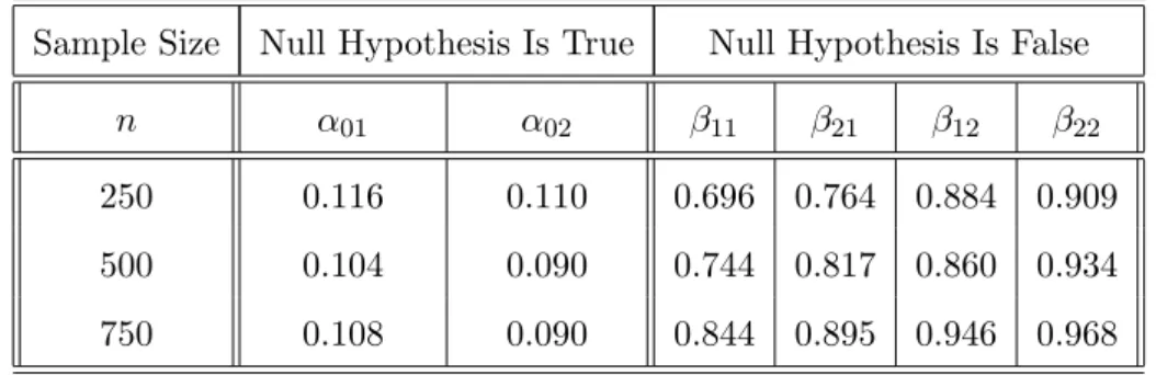
Sample Size Null Hypothesis Is True Null Hypothesis Is False
n α01 α02 β11 β21 β12 β22
250 0.116 0.110 0.696 0.764 0.884 0.909 500 0.104 0.090 0.744 0.817 0.860 0.934 750 0.108 0.090 0.844 0.895 0.946 0.968
Tables 4.1–4.3 report comprehensive simulation results for both the sizes and power values of the proposed tests for models (4.3) and (4.4). Column 2 in each of Tables 4.1–4.3 shows that while the sizes for the test based on !h0cv are comparable
with these given in column 3 based on !h0test, the power values of the test based on
!
hjtest in columns 6 and 7 are always greater than these given in columns 4 and 5
based on !hjcv. This is not surprising, because the theory shows that each of !hjtest is
chosen such that the resulting power function is maximized while the corresponding size function is under control by the significance level.
In addition, the test based on h!2test is almost uniformly more powerful than the
best based onh!1test, which is the second most powerful test. This is basically because
!
h2test is based on considering H1 with c2n = n−
7
18, which goes to zero slower than
c1n = n−
1 2
.
log log(n), and hence the distance between the alternative and the null is biggest in the former case (and therefore easier to detect). Meanwhile, the last columns of Tables 4.1–4.3 show that the test based on the bandwidth !h2test is still a
powerful test even though the bandwidth is proportional ton−1
6, which is the same as
the optimal bandwidth based on a cross–validation estimation method. This shows that whether an estimation–based optimal bandwidth may be used for testing depends on whether the bandwidth is chosen optimally for testing purposes.
We finally want to stress that the proposed test based on eitherh!1testorh!2test has
not only stable sizes even at a small sample size ofn = 250, but also reasonable power values even when the ‘distance’ between the null and the alternative has been made deliberately close at the rate of .n−1 loglog(n) = 0.060 forn= 500 for example. We
can expect that the test would have bigger power values when the ‘distance’ is made wider. Overall, Tables 4.1–4.3 show that the established theory and methodology is workable in the small and medium–sample case.
Example 4.1 discusses the small and medium–sample comparison results for the proposed test with either testing–based optimal bandwidth or estimation–based (CV) bandwidth. Example 4.2 below considers comparing the small and medium–sample
performance of the proposed test associated with the optimal bandwidth with some closely related nonparametric tests available in both the econometrics and statistics literature.
Example 4.2. Consider a linear model of the form
Yi =α0+β0 Xi+ei, 1≤i≤n = 250, (4.7)
where {Xi} is a sequence of independent random variables sampled from N(0,25)
distribution truncated at its 5th and 95th percentiles, and {ei} is sampled from one
of the three distributions: (i) ei ∼N(0,4); (ii) a mixture of Normals in which {ei} is
sampled from N(0,1.56) with probability 0.9 and from N(0,25) with probability 0.1; and (iii) the Type I extreme value distribution scaled to have a variance of 4. The mixture distribution is leptokurtic with a variance of 0.39, and the Type I extreme value distribution is asymmetrical.
This is the same example as used in Horowitz and Spokoiny (2001) for the compar-ison with some of the commonly used tests in the literature, such as the Andrews’ test proposed in Andrews (1997), the HM test proposed in H¨ardle and Mammen (1993), the HS test proposed in Horowitz and Spokoiny (2001) and the empirical likelihood (EL) test proposed in Chen, H¨ardle and Li (2003).
To compute the sizes of the test, choose α0 = β0 = 1 as the true parameters
and then generate {Yi} from Yi = 1 + Xi +ei under H0, and generate {Yi} from
Yi = 1 +Xi + 5τ φ
"X
i
τ
#
+ei under H1, where τ = 1 or 0.25, and φ(·) is the density
function of the standard normal distribution.
The kernel function used here isK(x) = 1516 (1−x2)2 I(|x| ≤1). Choosec
n = 5τ−1
and ∆(x) = φ(x τ−1) for the corresponding forms in (1.2). Forj = 1,2, letc
jn= 5τj−1
and ∆j(x) = φ(x τj−1) with τ1 = 1 and τ2 = 0.25. Let !hinew be the corresponding
version ofh!ew of (B.43) based on (cjn,∆j(x)) for j = 1,2.
In order to make a fair comparison, we use the same number of the bootstrap
M = 250 under H1 as in Table 1 of Horowitz and Spokoiny (2001). In Table 4.4
below, we add the size and power values to the last two columns for both the EL test and the proposed test–T!n
" !
hinew
#
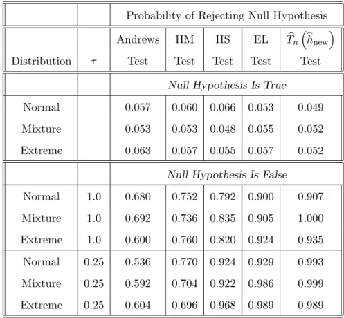
of this paper. The other parts of the table are obtained and tabulated similarly to Table 1 of Horowitz and Spokoiny (2001).
Table 4.4. Simulated size and power values at the 5% significance level Probability of Rejecting Null Hypothesis
Andrews HM HS EL T!n
" !
hnew
# Distribution τ Test Test Test Test Test
Null Hypothesis Is True
Normal 0.057 0.060 0.066 0.053 0.049 Mixture 0.053 0.053 0.048 0.055 0.052 Extreme 0.063 0.057 0.055 0.057 0.052
Null Hypothesis Is False
Normal 1.0 0.680 0.752 0.792 0.900 0.907 Mixture 1.0 0.692 0.736 0.835 0.905 1.000 Extreme 1.0 0.600 0.760 0.820 0.924 0.935 Normal 0.25 0.536 0.770 0.924 0.929 0.993 Mixture 0.25 0.592 0.704 0.922 0.986 0.999 Extreme 0.25 0.604 0.696 0.968 0.989 0.989
Table 4.4 shows that the proposed test has better power properties than any of the commonly used tests, while the size values are comparable with those of the com-petitors. The results further support the power–based bandwidth selection procedure proposed in Sections 2 and 3.
As discussed in the supplemental material, the proposed theory and methodology for model (1.1) can be applied to an extended model of the form
where σ(·) satisfying infx∈IRdσ(x) > 0 is unknown nonparametrically and {,i} is a
sequence of i.i.d. random errors with zero mean and finite variance. In addition, {,i}
and {Xj} are assumed to be independent for all 1 ≤ j ≤ i ≤ n. A special case of
model (4.8) is discussed in Example 4.3 below.
Example 4.3. This example examines the high frequency seven–day Eurodollar deposit rate sampled daily from 1 June 1973 to 25 February 1995. This provides us withn = 5505 observations. Let{Xi :i= 1,2,· · ·, n = 5505}be the set of Eurodollar
deposit rate data. Figures 4.1 and 4.2 below plot the data values and the conventional nonparametric kernel density estimator
! π(x) = 1 nh0cv n % i=1 K 1 x−Xi 0 hcv 2 respectively, where K(x) = √1 2πe− x2
2 and h0cv is the conventional normal–reference
based bandwidth given by
0 hcv = 1.06·n− 1 5 3 4 4 5 1 n−1 n % i=1 (Xi−X¯)2 with ¯X = 1 n n % i=1 Xi. (4.9)
Note that!bcv of (2.7),h!cv of (4.6) andh0cv of (4.9) are normally different from each
other. In the case where {Xi} follows an autoregressive model, they can be chosen
the same. Thus, they are chosen the same in this example.
It has been assumed in the literature (see, for example, A¨ıt–Sahalia 1996; Fan and Zheng 2003; Arapis and Gao 2006) that the Eurodollar data set {Xi} may be
modeled by a nonlinear time series model of the form
Yi =µ(Xi) +σ(Xi) ,i, 1≤i≤n, (4.10)
where Yi = Xi+1Λ−Xi, σ(·) >0 is unknown nonparametrically, and ,i ∼ N(0,Λ−1), in
which Λ is the time between successive observations. Since we consider a daily data set, this gives Λ = 1
1973 1977 1981 1985 1990 1994 0.05 0.10 0.15 0.20 0.25 Year
Eurodollar Interest Rate
Figure 4.1: Seven–day Eurodollar deposit rate, June 1, 1973 to February 25, 1995.
0.00 0.05 0.10 0.15 0.20 0.25
0
2
4
6
8
10
12
spot rate, rdensity function
Figure 4.2: Nonparametric kernel density estimator of the Eurodollar rate. On the question of whether there is any nonlinearity in the drift function µ(·), existing studies have provided no definitive answer. For example, A¨ıt–Sahalia (1996), and Arapis and Gao (2006) show that there is some evidence of supporting nonlin-earity in the drift on the one hand. On the other hand, existing studies, such as
Chapman and Pearson (2000), and Fan and Zheng (2003), suggest that nonlinearity may just be caused by estimation biases when using nonparametric kernel estimation. To further discuss whether the assumption on linearity in the drift is appropriate for the given set of data, we apply our test to propose testing
H01: µ(x) =µ(x;θ0) =β0(α0−x) versus H11: µ(x) =β1(α1−x)+cn∆(x) (4.11)
for some θj = (αj, βj) ∈ Θ for j = 0,1 and cn =
.
n−1log log(n), where Θ is a
parameter space in IR2 and ∆(x) is a continuous function.
It can be shown that the proposed test in Section 2 has an asymptotically equiv-alent version of the form:
0 Tn(h) = *n j=1 *n i=1,i&=je!j K "Xi−X j h # ! ei 6 2*n j=1 *n i=1e!2j K2 "Xi−X j h # ! e2 i , (4.12)
wheree!i =Yi−β!(α!−Xi), in which (α,! β!) is the pair of the conventional least squares
estimators minimizing *ni=1"Yi−β!(α! −Xi)
#2
.
As pointed out in the literature (Arapis and Gao 2006), T0n(h) is independent
of the structure of the conditional variance σ2(·). The kernel function used is the standard normal density function given by K(x) = √1
2πe
−x2
2 .
Let 0htest be the corresponding version of (B.43). It has been shown in Appendix
B below that 0 htest =a!− 1 2 1 t! −3 2 n , (4.13)
where !tn and a!1 are the same as in (B.43), in which c!(π) becomes
! c(π) = 1 n n % i=1 ! π2(Xi)σ!6(Xi)· 1 1 n n % i=1 ! π(Xi)σ!4(Xi) 2−3 2 (4.14) with ! σ2(Xi) = *n u=1K ( Xi−Xu 0hcv ) ! e2 u *n v=1K ( Xi−Xv 0hcv ) .
Let L1 = T0n(h0test) and L2 = T0n(h0cv). To apply the test Lj for each j = 1,2 to
test H01, we propose the following procedure for computing the p–value of Lj:
• Computee!i =Yi−β!(α!−Xi) and then generate a sequence of bootstrap
resam-ples {e!∗i} given by e!∗i = σ!(Xi) ,∗i, where {,∗i} is a sequence of i.i.d. bootstrap
resamples generated fromN(0,Λ−1) and σ!2(·) is defined as above.
• Generate Y!i∗ = β!(α!−Xi) +e!∗i. Compute the corresponding version L∗j of Lj
for each j = 1,2 based on{Y!∗
i }.
• Repeat the above steps M = 1000 times to find the bootstrap distribution of
L∗
j and then compute the proportion that Lj < L∗j for each j = 1,2. This
proportion is a simulated p–value of Lj.
Our simulation results return the simulated p–values of p!1 = 0.102 for L1 and
!
p2 = 0.072 for L2. While both of the simulated p–values suggest that there is no
enough evidence of rejecting the linearity in the drift at the 5% significance level, the evidence of accepting the linearity based onL1 is stronger than that based on L2.
As our test T0n(0htest) involves no estimation biases, the process of computing the
simulated p–values is quite robust. We therefore believe that this improved test further reinforces the findings of Chapman and Pearson (2000) and Fan and Zhang (2003) that there is no definitive answer to the question whether the short rate drift is actually nonlinear.
5. Conclusion
This paper has addressed the issue of how to appropriately choose the bandwidth parameter when using a nonparametric kernel–based test. Both the size and power properties of the proposed test have been studied systematically. The established theory and methodology has shown that a suitable bandwidth can be optimally chosen after appropriately balancing the size and power functions. Furthermore, the new
methodology has resulted in a closed–form representation for the leading term of such an optimal bandwidth in the finite–sample case.
Existing results (see, for example, Li and Wang 1998; Li 1999; Fan and Linton 2003; Gao 2007) show that this kind of nonparametric kernel test associated with a large sample critical value may not have good size and power properties. Our small and medium–sample studies in both the simulated and real–data examples have shown that the performance of such a test can be significantly improved when it is coupled with a power–based optimal bandwidth as well as a bootstrap simulated critical value. It is pointed out that the established theory and methodology has various ap-plications in providing solutions to some other related testing problems, in which nonparametric methods are involved. Future extensions also include dealing with cases where both Xi and ei may be strictly stationary time series.
Appendix A
This appendix lists the necessary assumptions for the establishment and the proofs of the main results given in Section 2.
A.1. Assumptions
Assumption A.1. (i)Assume that{ei}is a sequence of i.i.d. continuous random errors
withE[e1] = 0, 0< σ2 =E[e12] =σ2 <∞ andE[e61]<∞.
(ii) We assume that {Xi} is strictly stationary and α–mixing with mixing coefficient
α(t) being defined by
α(t) = sup{|P(A∩B)−P(A)P(B)|:A∈Ωs1, B∈Ω∞s+t} ≤Cα αt (A.1)
for alls, t≥1, where0< Cα<∞and 0< α <1are constants, andΩji denotes theσ–field
generated by {Xk :i≤k≤j}.
(iii) We also assume that {Xs} and {et} are independent for all 1 ≤ s ≤ t ≤ n. Let
π(·) be the marginal density such that 0 < $ π3(x)dx < ∞, and πτ1,τ2,···,τl(·) be the joint
probability density of (X1+τ1, . . . , X1+τl) (1 ≤ l ≤ 4). Assume that πτ1,τ2,···,τl(·) for all 1≤l≤4 do exist and are continuous and bounded.
(iv)Assume that the univariate kernel functionK(·)is a symmetric and bounded proba-bility density function. In addition, we assume the existence of bothK(3)(·), the three–time
convolution of K(·) with itself, and K2(2)(·), the two–time convolution ofK2(·) with itself.
(v) The bandwidth parameter h satisfies both limn→∞h= 0 and limn→∞nhd=∞.
Assumption A.2. (i) Let H0 be true. Then for any sufficiently small ε1 >0 and some
B1L>0 lim n→∞P "√ n||θ!−θ0||> B1L # < ε1,
where θ0 is the same as defined in (1.2).
(ii)Let H1 be true. Then for any sufficiently small ε2>0 and someB2L>0
lim n→∞P "√ n||θ!−θ1||> B2L # < ε2,
where θ1 is the same as defined in (1.2).
(iii)There exist some absolute constantsε3 >0and0< B3L<∞such that the following
lim n→∞P "√ n||θ!∗−θ!||> B3L|Wn # < ε3
holds in probability, whereθ!∗ is as defined in the Simulation Procedure above Theorem 2.1. (iv)Let mθ(x)be differentiable with respect to θand ∂m∂θθ(x) be continuous in bothx and
θ. In addition, E,"mθ0(X1) ∂θ # "mθ 0(X1) ∂θ #τ
-is a positive definite matrix, and
0<7 ++++ + + + + ∂mθ(x) ∂θ |θ=θ0 + + + + + + + + 2 π2(x)dx <∞.
Assumption A.3. (i) Let {∆n(x)} be a sequence of continuous functions such that
0<$∆2
n(x)π2(x)dx <∞.
(ii)Let Cn2 satisfy limn→∞n
√
hd C2
n=∞ and limn→∞n Cn6 = 0, where
Cn2 = $∆2 n(x)π2(x)dx σ2.2ν 2 $ K2(v)dv , in which ν2 =E8π2(X1)9<∞.
Assumptions A.1–A.3 are standard and justifiable conditions. Some detailed justifica-tions are given in Appendix C below.
A.2. Technical lemmas
Recall that using limn→∞nhd=∞
κn = √ hd"µ23K2(0) nhd + 4µ3 2ν3 3 K(3)(0) # σ3 n ≡ c1 √ hd+c 2 1 n√hd = c1 √ hd ( 1 +c2c−11 1 nhd ) ≈c1 √ hd. (A.2)
In order to establish some useful lemmas without including non–essential technicality, we introduce the following simplified notation:
aij = 1 n√hdσ n K (X i−Xj h ) , Ln(h) = n % i=1 n % j=1,&=i aijeiej, ρ(h) = √ 2K(3)(0) $ π3(u)du 3 1:7 π2(u)du 7 K2(v)dv 2−3 √ hd. (A.3)
We need the following lemmas; their proofs are given in Appendix C below.
Lemma A.1. Suppose that the conditions of Theorem 2.2(i) hold. Then for any h
sup x∈IR1 + + +P(Ln(h)≤x)−Φ(x) +ρ(h) (x2−1)φ(x) + + +=O"hd#. (A.4)
RecallLn(h) =*ni=1*jn=1,&=iei aijej as defined in (A.3) and let
Tn(h) = hd2 nσn n % i=1 n % j=1,&=i ! ei Kh(Xi−Xj) !ej = hd2 nσn n % i=1 n % j=1,&=i ei Kh(Xi−Xj) ej + h d 2 nσn n % i=1 n % j=1,&=i Kh(Xi−Xj) & m(Xi)−m!θ(Xi) ' & m(Xj)−m!θ(Xj) ' +2h d 2 nσn n % i=1 n % j=1,&=i ei Kh(Xi−Xj) & m(Xj)−mθ!(Xj) ' ≡ Ln(h) +Sn(h) +Dn(h), (A.5) whereSn(h) = h d 2 nσn *n i=1*nj=1,&=i Kh(Xi−Xj) & m(Xi)−m!θ(Xi) ' & m(Xj)−m!θ(Xj) ' and Dn(h) = 2 hd2 nσn n % i=1 n % j=1,&=i ei Kh(Xi−Xj) & m(Xj)−m!θ(Xj) ' . (A.6)
DefineL∗n(h),Sn∗(h) andDn∗(h) as the corresponding versions ofLn(h),Sn(h) andDn(h)
Lemma A.2. Suppose that the conditions of Theorem 2.2(i) hold. Then sup x∈IR1 + + +P∗(L∗n(h)≤x)−Φ(x) +ρ(h) (x2−1)φ(x)+++=OP " hd#. (A.7)
Lemma A.3. Suppose that the conditions of Theorem 2.2(i) hold. Then underH0
E[Sn(h)] = O "√ hd# and E[D n(h)] =o "√ hd#, (A.8) E∗[Sn∗(h)] = OP "√ hd# and E∗[D∗ n(h)] =oP "√ hd#, (A.9) E[Sn(h)]−E∗[Sn∗(h)] =OP "√ hd# and E[D n(h)]−E∗[D∗n(h)] =oP "√ hd# (A.10)
in probability with respect to the joint distribution of Wn, where E∗[·] =E[·|Wn].
Lemma A.4. Suppose that the conditions of Theorem 2.2(ii) hold. Then underH1
lim
n→∞E[Sn(h)] =∞ and nlim→∞
E[Dn(h)]
E[Sn(h)] = 0
. (A.11)
A.3. Proof of Theorem 2.1:
A.3.1. Proof of (2.10): Recall from (2.8) and (A.5)–(A.6) that
! Tn(h) = (Ln(h) +Sn(h) +Dn(h))· σn ! σn + oP "√ hd#, (A.12) ! Tn∗(h) = (L∗n(h) +Sn∗(h) +D∗n(h))·σn ! σ∗ n +oP "√ hd#, (A.13)
whereσn2,σ!n2 and σ!n∗2 are as defined in (2.4), (2.7) and (2.9) respectively.
In view of Assumption A.2 and Lemmas A.1–A.3, we may ignore any terms with orders higher than√hd and then consider the following approximations:
! Tn(h) = Ln(h) +E[Sn(h)] +oP( √ hd) and ! Tn∗(h) = L∗n(h) +E∗[Sn∗(h)] +oP "√ hd#. (A.14)
Let s(h) =E[Sn(h)] and s∗(h) =E∗[Sn∗(h)]. We then apply Lemmas A.1 and A.2 to
obtain that uniformly overx∈IR1,
P"T!n(h)≤x # = P"Ln(h)≤x−s(h) +oP "√ hd## (A.15) = Φ(x−s(h))−ρ(h)((x−s(h))2−1)φ(x−s(h)) +o"√hd# and P∗"T!n∗(h)≤x# = P∗"L∗n(h)≤x−s∗(h) +oP "√ hd## = Φ(x−s∗(h))−ρ(h)((x−s∗(h))2−1)φ(x−s∗(h)) +oP "√ hd#.