Feature selection and modelling methods for microarray data from acute coronary syndrome

Feature Selection and Modelling

Methods for Microarray Data from

Acute Coronary Syndrome

A thesis submitted to the University of Sheffield for the degree of Doctor of Philosophy

Adrian Alecu

Department of Automatic Control and Systems Engineering

i

Acknowledgements

I would like to thank my supervisors Professor Daniel Coca and Doctor Timothy Chico for the guidance offered throughout my years of research in Sheffield. I also would like thank Doctor Marta Milo for providing the data for this project. Many thanks go to my colleagues in Room 316 who made the PhD experience more enjoyable and rewarding. In particular, I would like to thank Krishnanathan Kirubhakaran, Dorian Florescu and Andrew Hills for all the work-related discus-sions as well as for being great friends in time of need.

A massive thanks to all my friends from Sheffield and abroad who helped me write some adventure chapters in my book of days. In particular I would like to thank Ines for always keeping in touch in spite of my countless attempts at taking refuge in work to escape her enthusiastic randomness. A big thank you goes to Alina and Hibo for all the philosophical debates, to Irina for the occasional social dances and to Krish and Mihai for all the sport activities.

Finally and most importantly, I would like to thank my mother, my sister, Cate-rina, and my brother, Marius, for the constant support offered in the years I have been away from home.

ii

Abstract

Acute coronary syndrome (ACS) represents a leading cause of mortality and mor-bidity worldwide. Providing better diagnostic solutions and developing therapeu-tic strategies customized to the individual patient represent societal and econom-ical urgencies. Progressive improvement in diagnosis and treatment procedures require a thorough understanding of the underlying genetic mechanisms of the disease. Recent advances in microarray technologies together with the decreasing costs of the specialized equipment enabled affordable harvesting of time-course gene expression data. The high-dimensional data generated demands for compu-tational tools able to extract the underlying biological knowledge.

This thesis is concerned with developing new methods for analysing time-course microarray gene expression data, focused on identifying differentially expressed genes, deconvolving heterogeneous gene expression measurements and inferring dynamic gene regulatory interactions. The main contributions include: a novel multi-stage feature selection method, a new deconvolution approach for estimat-ing cell-type specific signatures and quantifyestimat-ing the contribution of each cell type to the variance of the gene expression patters, a novel approach to identify the cellular sources of differential gene expression, a new approach to model gene expression dynamics using sums of exponentials and a novel method to estimate stable linear dynamical systems from noisy and unequally spaced time series data. The performance of the proposed methods was demonstrated on a time-course dataset consisting of microarray gene expression levels collected from the blood samples of patients with ACS and associated blood count measurements. The re-sults of the feature selection study are of significant biological relevance. For the first time is was reported high diagnostic performance of the ACS subtypes up to three months after hospital admission. The deconvolution study exposed features of within and between groups variation in expression measurements and identi-fied potential cell type markers and cellular sources of differential gene expression. It was shown that the dynamics of post-admission gene expression data can be ac-curately modelled using sums of exponentials, suggesting that gene expression levels undergo a transient response to the ACS events before returning to equi-librium. The linear dynamical models capturing the gene regulatory interactions exhibit high predictive performance and can serve as platforms for system-level analysis, numerical simulations and intervention studies.

Contents

Nomenclature xiii Acronyms xv 1 Introduction 1 1.1 Background . . . 1 1.2 Motivation . . . 2

1.3 Overview of the thesis . . . 4

2 Feature selection methods for microarray gene expression data 6 2.1 Introduction to microarray technology . . . 7

2.1.1 Glass slide cDNA microarrays . . . 7

2.1.2 High-density oligonucleotide microarrays . . . 8

2.2 Gene expression profiling using microarrays . . . 9

2.2.1 Experimental design . . . 9

2.2.2 Sample preparation . . . 9

2.2.3 Hybridization and washing . . . 10

2.2.4 Image acquisition . . . 10

2.2.5 Data pre-processing . . . 10

2.2.6 Data analysis . . . 13

2.3 Statistical hypothesis testing in microarray experiments . . . 13

2.3.1 Single hypothesis testing . . . 14

2.3.2 Multiple hypothesis testing . . . 15

2.3.3 Statistical significance and biological relevance . . . 18

2.4 Feature selection in machine learning . . . 19

2.4.1 Unsupervised filtering approaches for microarray data . . . . 21

2.4.2 Filters based on information theory . . . 24

2.4.3 Wrapper methods . . . 27

2.4.4 Embedded methods based on SVM . . . 30

2.5 Conclusions . . . 31 iii

iv Contents

3 Modelling methods for microarray gene expression data 33 3.1 Deconvolution of microarray gene expression data from

heteroge-neous tissues . . . 33

3.1.1 The linear deconvolution model . . . 34

3.1.2 Estimation of cell type-specific proportions . . . 35

3.1.3 Estimation of cell type-specific expression levels . . . 36

3.1.4 Joint estimation of cell type-specific proportions and expres-sion levels . . . 37

3.2 Modelling dynamic GRNs . . . 39

3.2.1 General properties of GRNs . . . 40

3.2.2 Boolean and probabilistic Boolean networks . . . 42

3.2.3 Dynamic Bayesian networks . . . 44

3.2.4 Linear state-space models . . . 45

3.3 Conclusions . . . 49

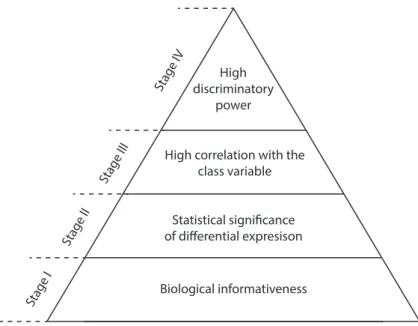
4 A novel multi-stage feature selection method for microarray gene expres-sion data 50 4.1 Stage I: Filtering uninformative genes . . . 52

4.2 Stage II: Gene subset selection using statistical tests . . . 53

4.2.1 The Welch’st-test . . . 53

4.2.2 The Wilcoxon’s rank-sum test . . . 54

4.2.3 pFDR control andq-value estimation . . . 55

4.3 Stage III: Gene subset selection using mRMR . . . 56

4.3.1 The CACC discretization algorithm . . . 56

4.4 Stage IV: Gene subset selection using SVMs . . . 58

4.5 Model selection and reliable performance evaluation . . . 60

4.5.1 The nested cross-validation design . . . 60

4.5.2 The multi-stage feature selection method . . . 62

4.6 Gene selection for ACS classification . . . 66

4.6.1 The ACS dataset . . . 66

4.6.2 Selection of differentially expressed genes between MI and UA 67 4.6.3 Selection of differentially expressed genes between NSTEMI and STEMI . . . 74

4.7 Conclusions . . . 79

5 A novel deconvolution method for microarray gene expression data 82 5.1 An orthogonal forward regression approach for microarray data de-convolution . . . 83

Contents v

5.3 Expression deconvolution of the genes differentiating between the ACS subtypes . . . 89 5.3.1 The CBC dataset . . . 89 5.3.2 Expression deconvolution of the genes differentiating MI from

UA . . . 90 5.3.3 Expression deconvolution of the genes differentiating NSTEMI

from STEMI . . . 96 5.4 Conclusions . . . 101 6 A novel approach for modelling stable GRNs 103

6.1 Nonlinear approximation of gene expression dynamics by sums of exponentials . . . 104 6.1.1 The gene expression model . . . 104 6.1.2 Parameter estimation using non-linear least squares . . . 106 6.1.3 Selecting the regularization parameter using the Morozov’s

discrepancy principle . . . 108 6.2 Modelling GRNs using linear dynamical systems . . . 109 6.2.1 Parameter estimation using non-linear least squares . . . 109 6.2.2 Selecting the regularization parameter by cross-validation . . 111 6.3 Estimating sparse GRNs . . . 112 6.4 Modelling GRNs for the diagnostic groups of ACS . . . 113

6.4.1 Modelling the regulatory interactions between the genes dif-ferentiating MI from UA . . . 113 6.4.2 Modelling the regulatory interactions between the genes

dif-ferentiating NSTEMI from STEMI . . . 117 6.5 Conclusions . . . 121

7 Conclusions 123

7.1 Summary and Conclusions . . . 123 7.2 Future work . . . 125

A Fundamentals of genetics 127

B Feature selection for ACS classification 132 C Deconvolution of microarray gene expression data 144 D Reconstruction of GRNs for the ACS subtypes 152

List of Figures

4.1 Hierarchical organization of the stage-specific forms of relevance . . 51 4.2 Nested cross-validation design of the multi-stage feature selection

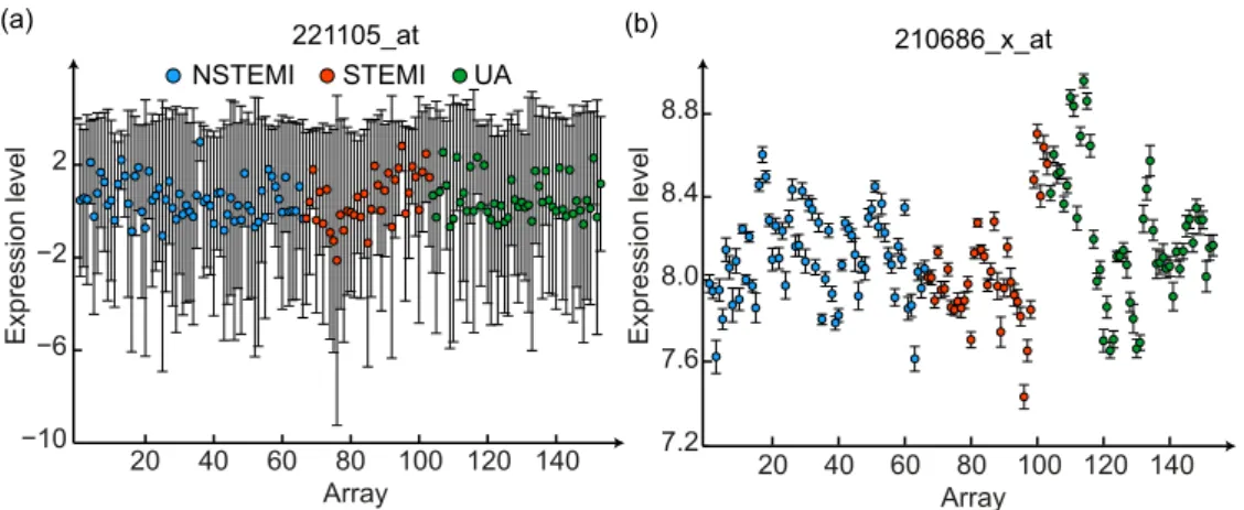
algorithm. . . 65 4.3 Expression levels across arrays for (a) a non-informative probe set

and (b) an informative probe set. The bars denote the technical variance of each measurement. . . 68 4.4 Mean densities (dotted lines) of the Hedges’gscores for the subsets

of gene selected using pFDR (Stage II) and mRMR (Stage III) in the external cross-validation loop. The continuous lines denote one standard deviation around the mean densities. . . 68 4.5 Hierarchical clustering of the group-specific expression averages of

the genes selected at Stage III in one fold of the external cross-validation loop. . . 69 4.6 Principal component analysis of the combined expression data of

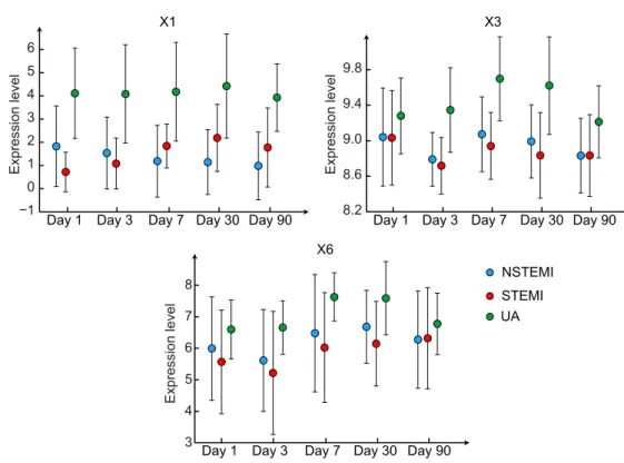
S_f. Dotted lines represent one standard deviation around the group-specific gene expression averages projected onto the principal com-ponents space. . . 71 4.7 Group-specific expression averages across visits for (a)X1(WASH1),

(b) X3 (C17orf103) and (c) X6 (OSBP2). The bars denote one

stan-dard deviation around the mean expression levels. . . 71 4.8 Principal component analysis of the combined expression data of

S∗

f. Dotted lines represent one standard deviation around the group-specific gene expression averages projected onto the principal com-ponents space. . . 74 4.9 Expression level across arrays for (a) a non-informative probe set

and (b) an informative probe set. The bars denote the technical variance of each measurement . . . 75

List of Figures vii

4.10 Mean density (dotted line) of the Hedges’gscores for the subsets of gene selected using pFDR (Stage II) in the external cross-validation loop. The continuous lines denote one standard deviation around the mean density. . . 75 4.11 Hierarchical clustering of the group-specific expression averages of

the genes selected at Stage II in one fold of the external cross-validation loop. . . 76 4.12 Principal component analysis of the combined expression data of

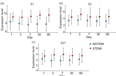
S_f. Dotted lines represent one standard deviation around the group-specific gene expression averages projected onto the principal com-ponents space. . . 77 4.13 Group-specific expression averages across visits for (a) X1

(HLA-DQB1), (b)X2(MAPK8Ip1) and (c)X21(LRRC37A). The bars denote

one standard deviation around the mean expression levels. . . 77 4.14 Principal component analysis of the combined expression data of

S∗_f. Dotted lines represent one standard deviation around the group-specific gene expression averages projected onto the principal com-ponents space. . . 79 5.1 Distributions of the CODs across visits for the models fitted on data

from the MI and UA groups using (a) the constrained OFR and (b) the unconstrained OFR. The lower and upper edge of the box repre-sent the 25th and 75th percentiles, respectively, while the whiskers extend to the most extreme points not considered outliers. . . 93 5.2 Cell type-specific contributions to the expression level of genes X1,

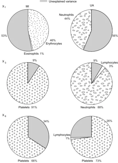
X3andX6in the MI and UA groups. . . 94

5.3 Distributions of the blood cell counts in the MI and UA groups . . . 95 5.4 Distributions of the CODs across visits for the models fitted on data

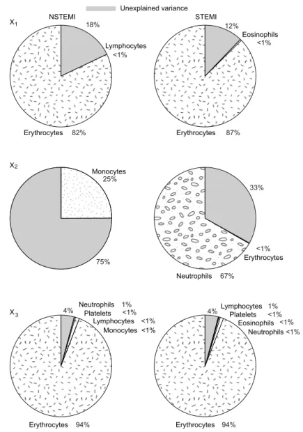
from NSTEMI and STEMI groups using (a) the constrained OFR method and (b) the unconstrained OFR method. . . 98 5.5 Cell type-specific contributions to the expression level of genes X1,

X2andX3in the NSTEMI and STEMI groups. . . 99

5.6 Distributions of the blood cell counts in the NSTEMI and STEMI groups . . . 100 6.1 Estimated dynamic profiles for (a) X1 (WASH1), (b) X3(C17orf103)

and (c)X6(OSBP2). The bars denote one standard deviation around

the group-specific gene expression averages. . . 114 6.2 Distributions of the prediction errors for the families of GRNs. . . . 116

viii List of Figures

6.3 Sparsity filters for the parameters of the GRNs associated with NSTEMI,

STEMI and UA . . . 117

6.4 Regulatory map for genes X1-X5 in the: (a) NSTEMI network, (b) STEMI network and (c) UA network. Each gene is represented by an unique colour. Regulatory connections sharing the colour of a gene point towards the genes that regulate it. The(∗)marks the regula-tory interactions with the largest magnitude that were removed by the sparsity filter. These connections were included to show at least one regulator per gene. . . 118

6.5 Estimated dynamic profiles for (a)X1(HLA-DQB1), (b)X2(MAPK8IP1) and (c) X21 (LRRC37A). The bars denote one standard deviation around the group-specific gene expression averages. . . 119

6.6 Distributions of the prediction errors for the families of GRNs . . . . 120

6.7 Sparsity filters for the parameters of the GRNs associated with NSTEMI and STEMI . . . 121

6.8 Regulatory map for genes X1-X5 in the: (a) NSTEMI network and (b) STEMI network. Each gene is represented by an unique colour. Regulatory connections sharing the colour of a gene point towards the genes that regulate it . . . 122

A.1 DNA double helix . . . 127

A.2 RNA hairpin loop . . . 128

A.3 The fundamental stages of protein biosynthesis . . . 128

A.4 Schematic representation of a GRN. Gene1 and Gene4 jointly reg-ulate the expression level (abundance of ribonucleic acid (RNA) and protein) of Gene5 through the protein complex assembled for their individual translation products (Protein1 and Protein4). The amount of Protein1 is regulated by Gene2 through RNA2 that binds to molecules of RNA1, preventing further protein translation. . . 129

A.5 Affymetrix GeneChip design . . . 130

A.6 Example of a gene (X1) with three inward connections (in-degree) and eleven outward connections (out-degree). X1 is regulated by X2,X3andX4 and regulates the expression level of genesX5−X15. 131 B.1 Group-specific expression averages across visits for genesX1−X18 in the MI vs. UA study. . . 135

B.2 Group-specific expression averages across visits for genesX19−X36 in the MI vs. UA study. . . 136

List of Figures ix

B.3 Group-specific expression averages across visits for genesX1−X15

in the NSTEMI vs. STEMI study. . . 141 B.4 Group-specific expression averages across visits for genesX16−X21

in the NSTEMI vs. STEMI study. . . 142 D.1 Estimated dynamic profiles for genes X1−X12 in the MI vs. UA

study. The bars denote one standard deviation around the group-specific gene expression averages . . . 153 D.2 Estimated dynamic profiles for genes X13−X20 in the MI vs. UA

study. The bars denote one standard deviation around the group-specific gene expression averages . . . 154 D.3 Dynamic profiles of the combined expression levels for genesX₁∗−

X∗₁₂ selected by l1-StaR in the MI vs. UA study. The bars denote

one standard deviation around the group-specific gene expression averages . . . 156 D.4 Dynamic profiles of the combined expression levels for genesX₁₃∗ −

X∗₂₀ selected by l1-StaR in the MI vs. UA study. The bars denote

one standard deviation around the group-specific gene expression averages . . . 157 D.5 Gene regulatory network for genes X1-X20 in the NSTEMI group.

Each gene is represented by an unique colour. Regulatory connec-tions sharing the colour of a gene point towards the genes that reg-ulate it. The (∗)marks the regulatory interactions with the largest magnitude that were removed by the sparsity filter. These connec-tions were included to show at least one regulator per gene. . . 158 D.6 Gene regulatory network for genes X1-X20 in the STEMI group.

Each gene is represented by an unique colour. Regulatory connec-tions sharing the colour of a gene point towards the genes that reg-ulate it. The (∗)marks the regulatory interactions with the largest magnitude that were removed by the sparsity filter. These connec-tions were included to show at least one regulator per gene. . . 159 D.7 Gene regulatory network for genesX1-X20 in the UA group. Each

gene is represented by an unique colour. Regulatory connections sharing the colour of a gene point towards the genes that regulate it. The (∗)marks the regulatory interactions with the largest mag-nitude that were removed by the sparsity filter. These connections were included to show at least one regulator per gene. . . 160

x List of Figures

D.8 Estimated dynamic profiles for genes X1-X12 in the NSTEMI vs.

STEMI study. The bars denote one standard deviation around the group-specific gene expression averages . . . 161 D.9 Estimated dynamic profiles for genes X13-X21 in the NSTEMI vs.

STEMI study. The bars denote one standard deviation around the group-specific gene expression averages . . . 162 D.10 Dynamic profiles of the combined expression levels for genes X₁∗−

X₁₁∗ selected by l1-StaR in the NSTEMI vs. STEMI study. The bars

denote one standard deviation around the group-specific gene ex-pression averages. . . 164

List of Tables

2.1 Possible outcomes from mhypothesis tests . . . 15

4.1 Quanta matrix for featureXj . . . 57

4.2 Amount of patients by visits and diagnostic groups . . . 67

4.3 Classification performance of the subsets of genesSIV _{. . . . 70}

4.4 l1-STaR parameters . . . 72

4.5 l1-STaR performance and number of selected genes for eachη . . . . 72

4.6 Classification performance of the subsets of genes selected by l1 -StaR . . . 73

4.7 Classification performance for the subsets of genesSIV _{. . . . 76}

4.8 l1-STaR performance and number of selected genes for eachη . . . . 78

4.9 Classification performance of the subsets of genes selected byl1-StaR 78 5.1 Amount of arrays associated with CBC data . . . 90

5.2 Average count for each blood cell in the diagnostic groups of ACS . 90 5.3 Gene differentially expressed between NSTEMI and STEMI . . . 91

5.4 Correlation between blood cell counts in the MI and UA groups . . 92

5.5 Gene differentially expressed between NSTEMI and STEMI . . . 96

5.6 Pairwise correlations between blood cell in the NSTEMI and STEMI groups . . . 97

5.7 Gene differentially expressed between NSTEMI and STEMI . . . 101

6.1 Eigenvalues of the GRNs associated with the ACS subtypes . . . 115

6.2 Eigenvalues of the GRNs associated with NSTEMI and STEMI . . . 120

B.1 Sample of estimated gene expression levels . . . 133

B.2 Standard errors of the estimated gene expression levels listed in Table B.1 . . . 134

B.3 Differentially expressed genes between the MI and UA groups se-lected by the multi-stage feature selection method . . . 137

xii List of Tables

B.4 Optimal classifier parameters for the MI vs. UA study . . . 138 B.5 Differentially expressed genes between the MI and UA groups

se-lected byl1-StaR . . . 139

B.6 Differentially expressed probe sets between the NSTEMI and STEMI groups selected by the multi-stage method . . . 140 B.7 Optimal classifier parameters for the NSTEMI vs. STEMI study . . . 140 B.8 Differentially expressed genes between the NSTEMI and STEMI

groups selected byl1-StaR . . . 143

C.1 Cell type-specific contributions to the variance of the genesX1−X18

in the MI group . . . 145 C.2 Cell type-specific contributions to the variance of the genes X19−

X36 in the MI group . . . 146

C.3 Cell type-specific contributions to the variance of the genesX1−X18

in the UA group . . . 147 C.4 Cell type-specific contributions to the variance of the genes X19−

X36 in the UA group . . . 148

C.5 Cell type-specific contributions to the variance of the genesX1−X21

in the NSTEMI group . . . 149 C.6 Cell type-specific contributions to the variance of the genesX1−X21

in the STEMI group . . . 150 C.7 Amount of genes expressed in each cell type in the MI and UA groups151 C.8 Amount of genes expressed in each cell type in the NSTEMI and

STEMI groups . . . 151 D.1 Goodness of fit for the genes differentiating MI from UA . . . 155 D.2 Goodness of fit for the genes differentiating NSTEMI from STEMI . 163

Nomenclature

A list of the variables and notation used in this thesis is defined below. The def-initions and conventions set here will be observed throughout unless otherwise stated. For a list of acronyms, please consult page xv.

#(S) cardinality of setS

α significance level for hypothesis testing

∩ set intersection

∪ set union

∆t sampling time

det determinant of a matrix

dimV dimension of the vector spaceV

∅ empty set

η regularization parameter

γ rejection region in statistical hypothesis testing κ(·,·) kernel function for the SVM classifier

kerV kernel of the vector spaceV

λ eigenvalue

[x]₊ maximum ofx and 0

C complex numbers

R+ positive real numbers

Z integer numbers

xiv List of Tables

N(µ,Σ) normal distribution with meanµand covarianceΣ

U[a,b] uniform distribution with support[a,b]

\ set difference

var(x) variance of the random variablex

> matrix transpose

$ tolerance parameter for the OFR algorithm

I identity matrix

C box constraint for the SVM classifier

E[·] expected value operator

p p-value

P(x) probability density function of the random variablex

Acronyms

A/M/P Absent/Marginal/Present. 22, 23

ACS acute coronary syndrome. ii, 1–3, 5, 52, 66, 80, 81, 89, 90, 101, 113, 114, 121, 123–126

AIC Akaike information criterion. 37 ANOVA analysis of variance. 125 BDe Bayesian Dirichlet equivalent. 45 BIC Bayesian information criterion. 45

BNRC Bayesian network and nonparametric regression criterion. 45 CACC class-attribute contingency coefficient. 56–58

CBC complete blood count. 89–91, 97 cDNA complementary DNA. 7–10, 31, 129

CMIM conditional mutual information maximization. 26 COD coefficient of determination. 43, 85, 92, 97, 101, 102 cRNA complementary RNA. 10, 129

csSAM cell type-specific significance analysis of microarrays. 37 DISR double input symmetrical relevance. 27

DNA deoxyribonucleic acid. 127–129 DrSVM doubly regularized SVM. 31 ECG electrocardiogram. 2

xvi Acronyms

EM expectation maximization. 45–47

FARMS factor analysis for robust microarray summarization. 12, 13, 23, 53 FDR false discovery rate. 16–18, 87

FWER family-wise error rate. 15–18 GCV generalized cross-validation. 112 GEO Gene Expression Omnibus. 35

GRN gene regulatory network. 3–5, 33, 39–41, 44, 47–49, 103, 104, 109–113, 115– 119, 121, 124, 126, 129

I/NI informative/non-informative. 23, 24, 53 IM ideal mismatch. 12

JMI joint mutual information. 27, 32

LASSO least absolute shrinkage and selection operator. 40 LCM laser capture micro-dissection. 34, 35

LDA linear discriminant analysis. 21, 28 LOOCV leave-one-out-CV. 61

MAS 5.0 Affymetrix microarray suite 5.0. 11, 12, 22 MCMC Markov chain Monte Carlo. 38

MI myocardial infarction. 2, 3, 66–70, 78, 82, 89–92, 94, 96, 113, 114, 118, 125 MID mutual information difference. 26, 56, 80

MIFS mutual information based feature selection. 26 MIQ mutual information quotient. 26, 56, 80

MM mismatch. 8, 11–13, 22

mRMR minimum redundancy - maximum relevance. 26, 27, 32, 50, 56, 80, 125 mRNA messenger ribonucleic acid. 6, 9, 10, 23, 34, 128, 129

Acronyms xvii

multi-mgMOS multi-chip modified gamma Model for Oligonucleotide Signal. 12, 13, 52, 66, 79, 108

NB naive Bayes. 21, 27

NSTEMI non-ST elevation MI. 2, 3, 66, 69, 74–78, 82, 89, 91, 96, 97, 100, 113, 115, 116, 119

OFR orthogonal forward regression. 4, 82, 83, 85–87, 89, 92, 97, 98, 101, 124 OLS orthogonal least squares. 83, 84, 87, 88

PCR polymerase chain reaction. 7, 8

pFDR positive false discovery rate. 17, 18, 32, 53, 55, 80, 89 PM perfect match. 8, 11–13, 22, 23

PPLR probability of positive log ratio. 66 RFE recursive feature elimination. 30, 50 RMA robust multi-array average. 11–13

RMSPE root mean square percentage error. 116, 119 RNA ribonucleic acid. viii, 9, 66, 92, 101, 127–129 RT reverse transcriptase. 9, 10

STEMI ST elevation MI. 2, 3, 66, 69, 74–78, 82, 89, 91, 96, 97, 100, 113, 115, 116, 119

SVM support vector machine. 21, 28–32, 50, 58, 59, 72, 80, 125 SVM-RFE SVM with recursive feature elimination. 30, 50, 51

Chapter 1

Introduction

1.1

Background

The cellular pathways are regulated by complex functional interactions between genes. Abnormal levels of gene expression can indicate irregularities in cell func-tioning (e.g. diseases) induced by changes in gene regulatory interactions (Emils-son et al., 2008, Schadt et al., 2005). Gene expression profiling and analysis can pro-vide a deeper understanding of current diseases and assist personalized medicine to develop more efficient treatments tailored to the individual patients that ac-count for their unique genetic variations.

Gene expression profiling is performed using high-throughput screening tech-nologies such as microarrays, which allow for a genome-wide interrogation of the cell’s transcriptional activity. Depending on the objectives of the experiment, the high dimensionality of the microarray data can raise significant computational and theoretical challenges in terms of extracting the underlying biological knowledge. Responses to these challenges emerged from various disciplines such as applied mathematics, computers science, statistics and engineering which recently defined the multidisciplinary field of computational biology. This field became the work-ing ground for uncoverwork-ing the dynamics of diseases that eluded the traditional medical understanding.

One such disease and a leading cause of mortality worldwide is acute coronary syndrome (ACS), which accounts for more than 2.5 million hospitalisations each year (Grech and Ramsdale, 2003). ACS is caused by the rupture of an atheroscle-rotic plaque (accumulation of fatty and calcium substances on an artery wall), resulting in a complete, partial or intermittent obstruction of blood supply to the heart (Libby, 2001). This occurs when inflammatory reactions caused by the in-teraction between macrophages and low density lipoproteins (molecules in charge

2 1.2. Motivation

with the transport of cholesterol) trigger plague erosion or disruption (Davies, 2000). The resulting thrombosis (blood clot inside a blood vessel) decreases the oxygen supply to the heart and leads to chest pain or to myocardial infarction (MI). Major factors influencing the risk of ACS consists of age, sex, family history, smoking, alcohol consumption and type II diabetes (Overbaugh, 2009).

ACS is usually diagnosed by performing an electrocardiogram (ECG) test. This test allows the doctor to evaluate the heart’s electrical activity. Abnormal changes in the electrical activity patterns can be used to identify the three subtypes of ACS: non-ST elevation MI (NSTEMI), ST elevation MI (STEMI) and unstable angina (UA), which differ with respect to severity, duration and treatment (Overbaugh, 2009). The ECG test is often insufficient to accurately diagnose MI due to other medical conditions presenting ST deviations (Ahmad and Sharma, 2012). To assist and improve the diagnostic accuracy of MI, cardiac markers such as troponin, cre-atine kinase-MB and myoglobin are often measured. The markers rise in response to the ischemic event and return to baseline in 24 hours (myoglobin), 72 hours (creatine kinase-MB) or are cleared from circulation up to 14 days (troponin) after infarction (Ahmad and Sharma, 2012).

The symptoms of the disease, ranging from chest pain (with or without radia-tion to the left arm, back or neck), nausea, shortness of breath and fatigue, emerge when the atherosclerotic process is already well-developed and often result in critical coronary events. Recent figures show that in UK only, every four minutes someone suffering from ACS is admitted to hospital and over 90 people die every day from a heart attack (Associates, 2011), a large proportion of deaths occurring before the patients reach a hospital. Treatment procedures consisting of drug ther-apy, percutaneous cardiac intervention or coronary artery bypass grafting, induce substantial healthcare expenditure and economic losses, amounting to £3.6 billion in 2009-10 (Associates, 2011). The high mortality rate and the current economic burden of the disease highlight the urgency to acquire a better understanding of the genetics of ACS in order to improve diagnosis and treatment solutions.

1.2

Motivation

The increasing affordability of gene expression profiling services empowered time-course studies of ACS (Kiliszek et al., 2012, Silbiger et al., 2013). These studies focused on identifying genes serving as new biomarkers for the early stages of the disease and for monitoring cardiac ischemic recovery. Extending the tempo-ral range of the gene expression studies together with the spectrum of biological questions addressed using the resulted time-course data could greatly advance

Chapter 1. Introduction 3

our understanding of the disease.

This thesis addresses three fundamental challenges related to the genetics of ACS from a computational biology perspective. The first challenge consists of identifying genes differentiating between MI (NSTEMI and STEMI) and UA pa-tients, and between NSTEMI and STEMI papa-tients, up to three months after hos-pital admission given time-course microarray data measured from blood samples. These findings could reveal novel cardiac markers for long term diagnosis or in-dicate genes explaining the genetic predisposition to ACS.

The second challenge consists of identifying the blood cells expressing the genes discriminating between the ACS subtypes and quantifying their contribu-tion to the variability and abundance of the total gene expression measured. These findings could indicate sources of interindividual variability in the gene expres-sion patterns, reveal the cellular sources of differential gene expresexpres-sion or pinpoint cell type-specific markers (gene uniquely expressed only in particular cell types).

The third challenge consists of inferring the regulatory pathways between the genes distinguishing between the ACS subtypes. Models describing the dynamics of the gene regulatory networks (GRNs) could be used to make qualitative and quantitative predictions about the network’s behaviour under different conditions. Numerical simulations and intervention studies based on these networks could expose the underlying mechanisms of the disease and assist the development of more efficient treatments.

To address the first challenge, a novel feature selection method consisting of four stages is proposed. In the first stage, a new unsupervised filter is used to remove noisy and uninformative genes based on their biological and technical variance. The second stage uses standard test statistics to select differentially ex-pressed genes while accounting for the problems arising when simultaneously testing multiple hypotheses. The third stage adopts an information theoretic based criterion operating on discretized data to select genes highly correlated with the ACS subtypes and minimally correlated with each other. Data discretization is performed using a state-of-the-art discretization algorithm that accounts for the unequal number of patients in each diagnostic group of ACS. The final stage com-bines a search strategy with a state-of-the-art classifier to select a minimal subset of genes with the highest diagnostic performance. To provide an unbiased es-timate of the diagnostic performance and avoid the sources of bias incurred in feature selection and parameter estimation, the stages are embedded in a nested cross-validation framework.

To address the second challenge, a novel deconvolution method for microar-ray gene expression data is proposed. This method combines non-negative least

4 1.3. Overview of the thesis

square optimization with the orthogonal forward regression (OFR) approach pro-posed by Billings et al. (1988) to estimate positive cell type-specific expression levels and quantify their contribution to the variance of the gene expression pat-terns. To identify the cellular sources of differential gene expression, an approach for comparing the coefficients of two regression models is adopted from the econo-metrics literature. This approach consists of introducing interaction terms between the regressing variables and the covariates (diagnostic groups) into the deconvo-lution model and testing the significance of their coefficients using a Wald test (Wald, 1943).

To address the third challenge, a novel method to estimate stable linear dynam-ical systems from time course gene expression data is proposed. The approach exploits the particular form of the state transition matrix when the dynamical system has single eigenvalues. The parameters of the state transition matrix are estimated using a regularized nonlinear optimization approach incorporating sta-bility constraints. To generate enough gene expression data for reconstructing GRNs of arbitrarily large sizes, a new approach based on modelling gene expres-sion dynamics using sums of exponentials is proposed. This approach can handle unequally sampled time series data and accounts for the measurement noise.

1.3

Overview of the thesis

This thesis is organized as follows:

• Chapter 2 provides an in-depth review of feature selection methods for mi-croarray data widely used in computational biology. The chapter begins with an introduction to microarray technology followed by an overview of the central steps of a microarray experiment. Emphasis is put on the Affymetrix GeneChip format and associated data pre-processing methods. The chapter continues with an introduction to statistical hypothesis testing in microarray experiments and a review of the multiple comparison procedures. The re-lation between statistical significance and biological relevance is further dis-cussed. An introduction to feature selection in machine learning is presented setting the scene for an extensive review of the state-of-the-art methods used to remove noisy and uninformative genes and select subsets of highly rele-vant features.

• Chapter 3 provides a review of modelling methods for microarray data fo-cused on gene expression deconvolution and reconstruction of GRNs. The review of deconvolution methods highlights the biases induced by sample

Chapter 1. Introduction 5

heterogeneity in differential expression studies and discusses computational tools addressing different deconvolution problems. The review of GRN re-construction methods lists the biological properties of GRNs together with strategies to incorporate biological constraints into the modelling process. Three major modelling formalism are reviewed and their strengths and lim-itations are highlighted.

• Chapter 4 presents the novel multi-stage feature selection method for mi-croarray data. A comparative study of the performance of the novel method and another multi-stage approach is conducted on a time-course microarray dataset collected from patients suffering from ACS. The results report the comparable performance of the two approaches expressed in terms of dis-criminatory power of the selected genes and highlight the appropriateness of the novel method for biomarker discovery in time-course microarray studies.

• Chapter 5 introduces the novel deconvolution method together with the ap-proach to conduct cell type-specific differential expression analysis. These methods are applied on the genes discriminating between the subtypes of ACS to identify the cellular sources of differential expression and measure the increments to the proportion of explained gene expression variance asso-ciated with each cell type. Results from this study show high deconvolution performance for most of the genes and argue that features of interindividual variability specific to microarray data collected from blood samples are re-sponsible for the low variability captured by the deconvolution model in the case of some genes. The need to supplement cell type-specific differential expression analysis with information regarding the deconvolution perfor-mance is also formulated.

• Chapter 6 presents the novel approaches to model gene expression dynam-ics and reconstruct stable GRNs. Additionally, a method to obtain sparse topologies for the estimated GRNs is discussed. Results show that mod-elling time course gene expression data using sums of exponentials ade-quately capture the dynamics of the genes differentiating between the ACS subtypes and that the novel method for GRN reconstruction estimates stable dynamical systems whose trajectories match extremely well the trajectories approximated using sums of exponentials. Sparse topological representa-tions for the estimated GRNs are derived and briefly discussed.

• Chapter 7 concludes the work done in this thesis and provides suggestions for future directions of research

Chapter 2

Feature selection methods for

microarray gene expression data

A major challenge in molecular biology is to uncover disease-specific genes that can be used as targets for treatment or as biomarkers for diagnosis. This challenge is traditionally approached through differential gene expression studies compar-ing the transcriptome abundance between case and control groups. The microar-rays technology is instrumental for this task, allowing the expression levels (abun-dance of messenger ribonucleic acid (mRNA) molecules) of tens of thousands of genes to be measured simultaneously. The high-dimensional data thus generated demands for computational tools able to remove genes that generate uninforma-tive signals and to select the genes that best discriminate between groups.

This chapter presents an introduction to microarray technology in Section 2.1 and an overview of the fundamental steps of a gene expression profiling experi-ment in Section 2.2. This is followed by a review of the statistical methods used to select differentially expressed genes in Section 2.3 and a survey of the supervised and unsupervised feature selection methods widely used in machine learning and bioinformatics in Section 2.4. Concluding remarks are given in Section 2.5. Fun-damental concepts of genetics introduced in this chapter and used throughout the thesis are discussed in more detail in Appendix A.

The supervised feature selection methods presented in this chapter address the problem of class comparison while the unsupervised approaches serve the task of removing noisy features. Unsupervised feature selection methods searching for the subspaces where data points cluster (class discovery) are outside the scope of this thesis. Comprehensive reviews of feature selection methods for clustering are provided by a number of authors including Parsons et al. (2004), Kriegel et al. (2009), Dash and Koot (2009) and Alelyani et al. (2013).

Chapter 2. Feature selection methods for microarray gene expression data 7

2.1

Introduction to microarray technology

The first step towards understanding the dynamics governing gene regulation was made by single-gene studies (Guan et al., 2010). The purpose of these studies was to characterize the selective activation and the functional role of individual genes. Recently, genome-wide-scale studies of genetic regulation became possible thanks to technological advances that enabled a global assessment of the cell’s transcriptional activity (Fryer et al., 2002). In particular, the microarray technology allowed for the expression of thousands of genes to be measured simultaneously using high-density and massively-parallel chips (Heller, 2002).

The microarray consists of oligonucleotides or polymerase chain reaction (PCR) products generated from purified complementary DNA (cDNA) templates, immo-bilized on a solid surface in an ordered arrangement (Falciani, 2007). Gene expres-sion profiling using microarrays relies on nucleic acid hybridization – the ability of single stranded nucleic acids to bind to complementary sequences (Strachan and Read, 2011). Complementarity between the nucleic acids immobilized on the array (probes) and the fluorescently labelled nucleic acids in the experimental sample (targets) allows for parallel quantification of the transcript abundance. Probes are incorporated on the array based on their sensitivity (strong complementarity with the target sequence) and specificity (absence of near-complementarity with non-target sequences) (Draghici et al., 2006, Kane et al., 2000). Variation in sensitivity and specificity among microarrays can be tracked down to fabrication technology. Microarrays are manufactured using two different technologies: spotting PCR products of cDNA templates on a glass surface (glass slide cDNA microarrays) (Duggan et al., 1999) or in situ synthesis of oligonucleotides (high-density oligonu-cleotide microarrays) (Lipshutz et al., 1999). The first manufacturing method is usually adopted within single facilities or laboratories; the second method is adopted by commercial companies. In what follows, the fabrication protocols of the glass slide cDNA microarrays and high-density oligonucleotide microarrays are presented with emphasis on the Affymetrix GeneChip format. Advantages and disadvantages of each technology are further discussed.

2.1.1 Glass slide cDNA microarrays

The first step in cDNA microarrays fabrication consists of selecting the templates for the probes (cDNA fragments of hundreds to thousands bases long) from ge-nomic libraries. The templates are cloned and amplified using PCR. In the next step, the glass slide is coated with chemicals that restrict the spread of spotted probes and facilitate their immobilization to the surface. Purified PCR products

8 2.1. Introduction to microarray technology

representing specific genes are later deposited in a matrix format. This is ac-complished through highly accurate contact printing methods (physical contact between the metal pin of a robotic arm and the slide surface) or non-contact print-ing methods (ink-jet array printers). Finally, the glass slide is dried and kept at room temperature.

Glass slide cDNA microarrays are particularly appealing for their reduced fab-rication costs. They are also highly versatile platforms for gene expression pro-filing studies, allowing customization in terms of the probes that are arrayed on the slide. cDNA microarrays have high sensitivity but low specificity. Their re-producibility is affected by problems inherent to PCR product concentration and quality of PCR clones (Järvinen et al., 2004).

2.1.2 High-density oligonucleotide microarrays

The first step in high-density oligonucleotide microarrays fabrication consists of attaching covalent linker molecules with photolabile protecting groups on a quartz wafer. Light directed through a photolithographic mask produces deprotection at specific locations on the quartz. Next, a solution of single protected nucleotides is incubated with the quartz and chemical coupling occurs at the deprotected sites. Uncoupled nucleotides are washed away and the process is repeated by changing the photolithographic mask and the solution of nucleotides until oligonucleotides with desired lengths are synthesized (Pease et al., 1994).

The Affymatrix GeneChip format uses 25-mer oligonucleotides (25 bases in length) representing unique sequences of genes. Target abundance is measured using a collection of 11-20 probe pairs, called a probe-set. Each probe pair consists of a perfect match (PM) probe and a mismatch (MM) probe which is obtained from the PM probe by changing the middle nucleotide. The MM probes quantify back-ground and non-specific hybridization thus allowing PM values to be corrected for hybridization artefacts. Multiple probe sets can interrogate the same gene. This level of redundancy enables false-positives detection and improves signal-to-noise ratios (Lipshutz et al., 1999). A schematic representation of the Affymetrix GeneChip is shown in Figure A.5 of Appendix A.

High-density oligonucleotide microarrays have high reproducibility. Consis-tency in fabrication protocols guarantees that the same gene profiling platform is used across experiments. Oligonucleotides have high specificity but low sensi-tivity. However, Affymetrix GeneChips achieve an optimal balance between high sensitivity and specificity through MM control probes. This additional level of in-formation improves the quality of the gene expression measurements thus increas-ing the robustness of genome-wide expression studies results (Affymetrix, 2001).

Chapter 2. Feature selection methods for microarray gene expression data 9

One disadvantage of this technology is affordability – oligonucleotide microarrays are expensive platforms. The costs of the specialized equipment necessary for con-ducting a gene expression profiling experiment make this technology unavailable for many average size laboratories.

2.2

Gene expression profiling using microarrays

Gene expression profiling experiments typically involve the following steps: 1. Experimental design

2. Sample preparation

3. Hybridization and washing 4. Image acquisition (scanning) 5. Data pre-processing

6. Data analysis

These steps are discussed in more detail below.

2.2.1 Experimental design

Careful formulation of the questions to be addressed or hypothesis to be tested lies at the heart of properly conducted gene expression studies (Yang and Speed, 2002). The aims of the experiment influence the choice of the microarray platform (cDNA arrays, oligonucleotides arrays), the number of technical replicates (arrays hybridized with the same sample) or biological replicates (arrays hybridized with different individual samples from the population being studied) needed, and the tools necessary for data pre-processing and analysis. Crafting the experimental setup around clear objectives maximizes the information leveraged from the data whilst minimizing the efforts and the costs (Stekel et al., 2003).

2.2.2 Sample preparation

Sample preparation consists of extracting mRNA from frozen tissue (freezing pre-vents further degradation or production of RNA). Isolation of mRNA can be per-formed directly from the cells or through purification of total RNA extracted. After isolation, mRNA is converted to cDNA using reverse transcriptase (RT) and labelled with a fluorescent dye. Sample preparation for Affymetrix GeneChips

10 2.2. Gene expression profiling using microarrays

involves additional steps: isolated mRNA is linearly amplified before the RT re-action and the resulted cDNA is used to produce anti-sense complementary RNA (cRNA) which is fluorescently labelled. Detailed technical specifications of sam-ple preparation are provided by a number of authors including Mahadevappa and Warrington (1999) and Hegde et al. (2000).

2.2.3 Hybridization and washing

The labelled sample is poured onto the microarray and incubation follows (at high salt concentrations, presence of formamide and temperature of 42◦ C, or presence of an aqueous solution and temperature of 65◦C) to promote probe-target hy-bridization. After the microarray is removed from the incubation chamber, strin-gent washes are performed (at lower salt concentrations and room temperature) to remove non-specific and weak bindings. For high-quality gene expression pro-filing, the hybridization and washing solution must be evenly mixed and spread on the microarray (Freeman et al., 2000).

2.2.4 Image acquisition

The microarray is scanned to produce an image containing the fluorescence inten-sity of each probe. This stage consists of exciting the dye using a laser beam thus generating signals dependent on the quantity of target sample hybridized with each probe on the chip. Ideally, fluorescent signals should come only from targets that hybridized to their complementary probes. In practice, unwashed targets adhering to the slide, non-specific bindings, and other chemicals used for array preparation, hybridization and washing also generate fluorescent signals (Scharpf et al., 2007). These residual signals (background noise) need to be accounted for as they affect probe value calculations.

2.2.5 Data pre-processing

Processing of the raw intensities generated during scanning consists of the follow-ing steps:

1. Background correction 2. Normalisation

3. Summarization (Affymetrix GeneChips only) These steps are discussed in more detail below.

Chapter 2. Feature selection methods for microarray gene expression data 11

Background correction

The purpose of background correction is to adjust the probe intensities by remov-ing the background noise. Methods for estimatremov-ing and subtractremov-ing the background noise are microarray technology dependent.

For cDNA microarrays, an unbiased estimate of the probe-specific background can be calculated from the local neighbourhood surrounding the probe by taking the mean of the pixel intensity values. The standard correction approach consists of subtracting the local background from the raw intensity values (Yin et al., 2005). To correct for negative adjusted intensities resulting from this approach, Edwards (2003) proposed a method that uses subtraction only when the difference exceeds a certain threshold; otherwise a smooth monotonic function that is linear on the log-scale with respect to the raw probe intensities is used. Yang et al. (2002) pro-posed sampling the probe-specific background at the probe nominal location from a background image estimated using morphological operations. This approach re-sults in less variable background adjusted intensities. Ritchie et al. (2007) provides a comparison of background correction methods for cDNA microarrays and their effect on identifying differentially expressed genes.

For oligonucleotide microarrays, the high-density of the chip prohibits the use of local neighbourhood methods. Instead, the MM control probes, which are adja-cent to their PM probes, can be used for background correction. Two widely used background correction methods are integral parts of Affymetrix microarray suite 5.0 (MAS 5.0) (Affymetrix, 2002) and robust multi-array average (RMA) (Irizarry et al., 2003).

The MAS 5.0 background correction method splits the chip into 16 rectangular zones of equal size. Zone-specific background and noise are taken as the mean and standard deviation of the lowest 2% probe intensities. For each probe, background and noise are calculated as weighted averages of the zone-specific background and noise signals, respectively. Probe intensities are adjusted by subtracting their back-ground unless the difference leads to a value less than the probe-specific noise, in which case the raw intensity is replaced by the noise.

The RMA background correction assumes the observed PM values within a probe set follow a linear additive model consisting of an exponentially distributed true signal and a normally distributed background. The adjustment procedure consists of replacing the PM intensity with the expected value of the true signal (which depends on the particular PM being adjusted, PM values above their mode and MM below their mode).

12 2.2. Gene expression profiling using microarrays

Normalization

The purpose of normalization is to adjust for systematic biases in sample collec-tion (Fentz et al., 2004), hybridizacollec-tion (Han et al., 2006), labelling (Gregory Cox et al., 2004) and scanning (Bengtsson et al., 2004) so that unbiased comparisons can be made across technical and biological replicates. Robust and widely used normalization methods vary from global normalization (Stafford, 2012) to quantile normalization (Bolstad et al., 2003) and lowess normalization (Smyth and Speed, 2003).

Global normalization consists of multiplying the probe intensities of each ar-ray with an arar-ray-specific scaling factor to adjust the mean or the median intensity values of the arrays; quantile normalization consists of transforming the distribu-tions of the array-specific intensities to have identical statistical properties; lowess normalization consists of removing the dependency of the log₂ ratio values on the intensity using locally weighted linear regression analysis. Normalization is a growing field which generated a consistent amount of literature. Comprehensive reviews are provided by a number of authors including Quackenbush (2002) and Bilban et al. (2002).

Summarization

The purpose of summarization is to estimate probe set expression levels from asso-ciated probe-pair intensities. Summarization methods are divided into two major categories: single-chip methods (summarization is performed for each array inde-pendently) and multi-chip methods (summarization is performed by borrowing information across arrays).

One of the most widely used single-chip methods is MAS 5.0 which provides for each probe set a robust average of the differences between the PM values and the associated ideal mismatch (IM) values. The IM value is equal to the MM value if MM<PM and is slightly less than the PM value (according to some adjustment formula) if MM>PM. Subtraction of MM values from PM values can induce bias in probe set level summarization (Irizarry et al., 2003) as MM probes also measure specific hybridization (Wu et al., 2004b) and can often exceed the values of the PM probes (effect observed in about one third of the probe-sets) (Naef et al., 2002). In addition, the PM and MM intensities vary in probe-specific ways (Li and Wong, 2001). These factors confounding accurate probe-set level summarization are not accounted for by MAS 5.0.

Multi-chip methods such as RMA, factor analysis for robust microarray sum-marization (FARMS) (Hochreiter et al., 2006) and multi-chip modified gamma

Chapter 2. Feature selection methods for microarray gene expression data 13

Model for Oligonucleotide Signal (multi-mgMOS) (Liu et al., 2005) adjust for the systematic differences in probe hybridization affinities. RMA assumes the log₂ transformed PM intensities follow a linear additive model consisting of the true probe set level, probe pair affinity effect and independent and identically dis-tributed error term. FARMS assumes the log₂ transformed PM intensities follow a factor analysis model consisting of the normally distributed true signal and nor-mally distributed noise. Finally, multi-mgMOS uses a probabilistic model with gamma distributed PM and MM values that additionally accounts for the MM probes measuring specific hybridization. This method returns the estimated probe set levels and the uncertainties (standard errors) around these estimates, which are particularly useful for downstream analyses adopting a Bayesian framework.

2.2.6 Data analysis

The pre-processed data is analysed to extract biologically-relevant information. Analysis methods are purpose-specific and the choice of the algorithms influences the quality of the results which are usually based on a list of selected genes. These genes need to be enriched with functional information (molecular functions and biological processes associated with the genes) in order to strengthen the under-standing of the biological process being studied.

Functional annotation can be performed using Gene Ontology (Consortium et al., 2004) which unifies functional information in highly interconnected struc-tures and under a common nomenclature. If valuable knowledge was gained by addressing the questions or testing the hypothesis of the experiment, the data is published following carefully defined standards (Brazma et al., 2001) into a public repository (Gardiner-Garden and Littlejohn, 2001).

2.3

Statistical hypothesis testing in microarray experiments

Statistical hypothesis testing is concerned with making inference about a statistical population given information from a random statistical sample (measured data). In the arena of differential gene expression studies, statistical hypothesis testing consists of assessing the quality of the evidence provided by the data against the claims of no differential expression.

Section 2.3.1 introduces the terminology of statistical testing and presents the single hypothesis testing scenario. This will lay the foundations for a discussion of multiple hypothesis testing and a review of multiple comparison correction methods in Section 2.3.2. Finally, a discussion on the relation between statistical

14 2.3. Statistical hypothesis testing in microarray experiments

significance and biological relevance is presented in Section 2.3.3, highlighting the need to supplement statistical findings with information from effect size measures.

2.3.1 Single hypothesis testing

In a single hypothesis testing scenario, given a statistic that quantifies an effect (or difference) in the sample data through a numerical summary T, one tests a null hypothesis (absence of an effect) against an alternative hypothesis (presence of the effect) at a chosen significance level α (commonly 0.05 or 0.01). If the p

-value i.e. the probability (under the null hypothesis) of observing a statistic at least as extreme as T is less than α, the null hypothesis is rejected in favour of

the alternative hypothesis; otherwise, one fails to reject the null hypothesis or equivalently concludes the data provides no reliable evidence against the null hypothesis.

Statistics commonly applied in differentially gene expression studies are di-vided into two major categories: parametric methods (distributional assumptions are made about the data) and non-parametric methods (no distributional assump-tions are made). The Welch t-test (Welch, 1947) and the Wilcoxon rank-sum test (Hollander et al., 2013) are two widely used parametric and non-parametric meth-ods, respectively. These methods are discussed in more detail in Chapter 4.

The known sampling distribution of these statistics under the null hypothe-sis allows for directp-values calculation. When the sampling distribution is not known a priori, it can be estimated using random permutation methods (Dudoit et al., 2002b, Pan, 2003). These methods are robust against outliers and repre-sent powerful alternatives to using known sampling distributions in studies with small sample size (Saeys et al., 2007). Chen et al. (2005) and Pan (2002) provide comprehensive reviews of the test statistics used in microarray studies.

There are two types of errors that can be committed when performing statisti-cal hypothesis testing: type I error and type II error. A type I error (false positive) is committed when rejecting a true null hypothesis; a type II error (false nega-tive) is committed when failing to reject a false null hypothesis. In the context of differential gene expression, type I error corresponds to erroneously calling a gene differentially expressed; a type II error corresponds to calling a gene non-differentially expressed when in fact it is non-differentially expressed. The false posi-tive rate is the rate at which true null hypotheses are called significant and equals the significance levelα. The false negative rate is the rate at which true alternative

hypotheses are called null. The single hypothesis testing scenario described above aims to control the false positive rate conditional on maximizing the power (1-false negative rate) of detecting an effect.

Chapter 2. Feature selection methods for microarray gene expression data 15

2.3.2 Multiple hypothesis testing

In a typical microarray experiment tens of thousands of genes are tested for dif-ferential expression. Controlling the false positive rate at a common significance levelα when simultaneously testing multiple hypotheses increases the chance of

committing type I errors (Dudoit et al., 2003). The significance level αmultiplied

by the number of hypothesis tested represents a conservative upper bound for the expected number of false positives. This bound is too large for microarray data.

By increasing the stringency of individual tests (lowering α) in an attempt to

decrease the expected number of Type I errors one instead decreases the power of the tests thus lowering the chances of detecting true differentially expressed genes. Since control of the false positive rate in the single hypothesis testing sense is unsatisfactory for multiple hypotheses testing, several generalizations of the Type I error rate were proposed together with procedures that control these error rates at a desired level α. These compound error measures and associated controlling

procedures are summarized within the setup of a multiple comparison experiment presented below.

Consider testing simultaneously mnull hypotheses Hi,i= 1, . . . ,m, at a com-mon significance threshold α. Assume the hypotheses are ordered in ascending

order of theirp-values p_i, which are associated with the independent test statistics

Ti. The possible outcomes of the multiple comparison tests are listed in Table 1. Specifically,Vrepresents the number of false positives,Urepresents the number of true positives,Trepresents the number of false negatives,Srepresents the number of true negatives and R represents the number of rejected null hypotheses. The quantities V, U, T and S are unobservable random variable; R is an observable random variable; the number of true null hypothesesm0 and the number of true

alternative hypothesesm1=m−m0 are unknown parameters.

Table 2.1: Possible outcomes frommhypothesis tests

Hypothesis Called significant Called non-significant Total

Null true V S m0

Alternative true U T m1

Total R m−R m

Historically, the first type I error rate proposed for multiple hypothesis testing was the family-wise error rate (FWER) (Shaffer, 1995):

FWER= P(V≥1) (2.1)

16 2.3. Statistical hypothesis testing in microarray experiments

of all hypotheses tested. Control of the FWER at a significance level α can be

achieved using various sequential p-value procedures reviewed by Dudoit et al. (2003) and Nichols and Hayasaka (2003). Presented below, in increasing order of their power, are three widely known representatives.

• The Bonferroni procedure (Simes, 1986) controls the FWER as follows: reject H_j forj=1, . . . , max

n

i|p_i ≤ α

m o

) (2.2)

• The Holm procedure (Holm, 1979) controls the FWER as follows: reject Hj forj=1, . . . , min

i|pi ≥ α m−i+1 −1 (2.3)

If there is no i for which the p-value inequality is satisfied, all hypotheses are rejected.

• The Hochberg procedure (Hochberg, 1988) controls the FWER as follows: reject Hj forj=1, . . . , max

i|pi ≤ α m−i+1 (2.4) If there is no i for which the p-value inequality is satisfied, mo hypotheses are rejected.

Controlling the FWER is concerned with guarding against the occurrence of any false positives. While this strict criterion is appropriate for studies where few true alternatives are expected, it is far too stringent for differential gene expression studies where the presence of an effect is manifested through more than one or two genes. In general, when controlling the FWER the power decreases with increasing number of hypothesis being tested (Storey, 2002).

Instead of controlling the probability of making at least one Type I error, one may be interested in making as many significant findings as possible while con-trolling the proportion of false positives. This problem was address by Benjamini and Hochberg (1995) who proposed controlling the false discovery rate (FDR):

FDR=E V R R >0 P(R>0) (2.5) as follows:

reject Hj forj=1, . . . , max

i|pi ≤ i mα (2.6) The FDR represents the expected proportion of Type I errors among the rejected null hypotheses times the probability of making at least one rejection.

Control-Chapter 2. Feature selection methods for microarray gene expression data 17

ling the FDR leads to a substantial gain in power over Bonferroni and Hochberg procedures for FWER control. This gain increases when the number of tested hy-pothesis or the number for true alternative hypotheses also increase (Benjamini and Hochberg, 1995). Storey (2002) signals that caution must be taken when con-trolling the FDR at a significance level αas in the case when null hypothesis are

rejected, one really controls the FDR at levelα/P(R>0).

The previous methods relied on setting the significance levelαprior to estimating

the rejection region for the p-values. The appropriateness of this approach is conditional upon the number of rejected hypothesis. Additionally, none of these methods uses information about the number of true null hypotheses m0 in the

data. To address these issues, Storey (2002) proposed fixing the rejection regionγ

and then estimating the significance level α through control of the positive false

discovery rate (pFDR): pFDR(γ) =E V(γ) R(γ) R(γ)>0 (2.7) The pFDR cannot be controlled using sequential p-value approaches but needs to be estimated for the particular rejection regionγas follows:

\ pFDR_δ(γ) = mπˆ0(δ)γ #{p_i ≤γ} (2.8) where ˆ π0(δ) = #{pi >δ} (1−δ)m (2.9)

with δ ∈ [0, 1]representing a tuning parameter used to determine the estimated

fraction of true null hypotheses ˆπ0(δ). The bias of ˆπ0(δ) is the smallest when δ → 1 (Storey, 2002). Equation (2.9) shows that pFDR control takes into account

the information stored in the observed p-values to estimatem0/m.

Within the pFDR framework, Storey (2003) proposed theq-value as an individ-ual measure of significance analogous to the p-value. Theq-value of the statistic

Ti, given a set of nested rejection regionsΓcontainingTi is:

q(Ti) = inf {Γ:Ti∈Γ}

pFDR(Γ) (2.10)

The q-value of a statistic gives the pFDR obtained when rejecting any statistic at least as extreme as the one observed among all the hypotheses; the p-value gives the false positive rate when rejecting any statistic at least as extreme as the observed statistic. A fundamental difference between theq-value and the p-value

18 2.3. Statistical hypothesis testing in microarray experiments

is that the former quantity accounts for the multiple comparisons carried out in parallel while the latter quantity does not. Thus thep-value carries no information about the set of more extreme statistics; theq-value directly provides a measure of strength for this set.

If the hypotheses are assumed to be independent, theq-value of a statistic T_i

can be expressed in terms of the associated pi as follows:

q(pi) = inf

γ≥pi

pFDR(γ) (2.11)

This allows for theq-values to be estimated as: ˆ

q(pi) = inf

γ≥pi \

pFDR(γ) (2.12)

Storey et al. (2004) proved the simultaneous conservative consistency of these es-timates. This means that the estimated q-values are simultaneously greater than or equal to the trueq-values for any rejection region. Thus, by calling significant statistics with q-value less than α one obtains a conservative point estimate for

the pFDR at significance levelα. When compared with the FDR control method

of Benjamini and Hochberg (1995), pFDR control provided greater power (Storey, 2002).

The multiple adjustment procedures listed above rely on the independence between the statistics Ti. Although microarray data violate this simplifying as-sumption through correlated gene expression levels, positive results were reported in differential gene expression studies adopting the multiple adjustment frame-work (Dudoit et al., 2002b, 2003, Efron and Tibshirani, 2002, Storey and Tibshirani, 2003). Methods that account for the dependence structure among statistics were proposed by Tusher et al. (2001) for FWER control and by Benjamini and Yeku-tieli (2001) and Storey et al. (2004) for FDR control. However, the area of multiple hypotheses testing exploiting the distribution of the statistics is still in its infancy and much research is needed to lay solid theoretical foundations.

2.3.3 Statistical significance and biological relevance

A common criticism addressed to statistical hypothesis testing is that statistical significance doesn’t necessarily translate into biological relevance (Lovell, 2013, Martínez-Abraín, 2008). The p-values don’t offer a quantitative measure of the magnitude of an effect but a qualitative measure of evidence against the null hy-pothesis. Thus, genes statistically significant can have a biologically irrelevant effect size.