Doctoral Dissertations Student Theses and Dissertations
2014
Longitudinal analysis of crash frequency data
Longitudinal analysis of crash frequency data
Mojtaba Ale Mohammadi
Follow this and additional works at: https://scholarsmine.mst.edu/doctoral_dissertations Part of the Civil Engineering Commons
Department: Civil, Architectural and Environmental Engineering Department: Civil, Architectural and Environmental Engineering Recommended Citation
Recommended Citation
Ale Mohammadi, Mojtaba, "Longitudinal analysis of crash frequency data" (2014). Doctoral Dissertations. 2498.
https://scholarsmine.mst.edu/doctoral_dissertations/2498
This thesis is brought to you by Scholars' Mine, a service of the Missouri S&T Library and Learning Resources. This work is protected by U. S. Copyright Law. Unauthorized use including reproduction for redistribution requires the permission of the copyright holder. For more information, please contact scholarsmine@mst.edu.
LONGITUDINAL ANALYSIS OF CRASH FREQUENCY DATA
by
MOJTABA ALE MOHAMMADI
A DISSERTATION
Presented to the Faculty of the Graduate School of the MISSOURI UNIVERSITY OF SCIENCE AND TECHNOLOGY
In Partial Fulfillment of the Requirements for the Degree
DOCTOR OF PHILOSOPHY in
CIVIL ENGINEERING
2014
Approved by
Dr. V.A. Samaranayake, Advisor Dr. Ghulam Bham, Co-Advisor
Dr. Ronaldo Luna Dr. Robert Paige Dr. Abhijit Gosavi
Copyright 2014 Mojtaba Ale Mohammadi
DEDICATION
I would like to dedicate this doctoral dissertation to my parents Nasser Ale Mohammadi and Maryam Rahimian, my two sisters Zakieh and Zahra, and my fiancée Mina Hadi whose continued love and support helped me much in completion of this process.
PUBLICATION DISSERTATION OPTION
This dissertation has been prepared in the styles utilized by the Transportation Research Record: Journal of Transportation Research Board and Journal of Analytic Methods in Accident Research. Pages 5-21 are published in Transportation Research Record: Journal of the Transportation Research Board; Pages 22-59 will be published at the Analytic Methods in Accident Research; Pages 60-85 is submitted to the
Transportation Research Record: Journal of Transportation Research Board. Appendices A and B and the Bibliography have been added for purposes normal to dissertation writing. Appendix C was also added last to incorporate the addressed comments of the committee members on the published papers.
ABSTRACT
This study comprises mainly of three papers. First, a systematic evaluation of the effects of Missouri’s Strategic Highway Safety Plan between 2004 and 2007 is presented. Negative binomial regression models were developed for the before-through-change conditions for the various collision types and crash severities. The models were used to predict the expected number of crashes assuming with and without the implementation of MSHSP. This procedure estimated significant reductions of 10% in crashes frequency and a 30% reduction for fatal crashes. Reductions in the number of different collision types were estimated to be 18-37%. The results suggest that the MSHSP was successful in decreasing fatalities.
Second, ten years (2002 - 2011) of Missouri Interstate highway crash data was utilized to develop a longitudinal negative binomial model using generalized estimating equation (GEE) procedure. This model incorporated the temporal correlations in crash frequency data was compared to the more traditional NB model and was found to be superior. The GEE model does not underestimate the variance in the coefficient estimates, and provides more accurate and less biased estimates. Furthermore, the autoregressive correlation structure used for the temporal correlation of the data was found to be an appropriate structure for longitudinal type of data used in this study.
Third, this study developed another longitudinal negative binomial model that takes into account the seasonal effects of crash causality factors using Missouri crash data. A GEE with autoregressive correlation structure was used again for model estimation. The results improve the understanding of seasonality and whether the magnitude and/or type of various effects are different according to climatic changes. It was found that the traffic volume has a higher effect in increasing the crash occurrence in spring and lower effect in winter, compared to fall season. The crash reducing effect of better pavements was found to be highest in spring season followed by summer and winter, compared to the fall season. The results suggest that winter season has the highest effect in increasing crash occurrences followed by summer and spring.
ACKNOWLEDGMENTS
Although this dissertation is individual work, I could have never reached the heights and explored the depth without the help and support of many people.
Firstly, I would like to thank my Advisor Dr. Samaranayake for instilling in me the qualities of being a good engineer who can plan for an objective and organize tasks and times in advance to achieve the goals. Dr. Sam has opened my eyes to the aspects of research which were not so vivid to me previously. He made me better understand that discussion of the results of an experiment is what makes it meaningful; always good to look at and argue the results and not simply see them as the possible outcomes.
I would like to thank my Co-advisor as well Dr. Bham who made me develop the required skills for being always hopeful in times of denial and disapproval by the higher ranked authorities, for changing my point of view toward people who demand without the appreciation of encouragement and motivation. He taught me to be self-inspired and love what I do.
I thank my committee members Dr. Ronaldo Luna, Dr. Robert Paige, and Dr. Abhijit Gosavi for their support. I also thank Karen White the graduate secretary of the civil engineering department for her many helpful tips.
I would like to thank Dr. Ezra Hauer for his father like and professional advice during a three-day workshop on safety performance functions. I also would like to thank Dr. Dominique Lord, Dr. Fred Mannering, Dr. Mohamed Abdel-Aty, and Dr.
Venkataraman Shankar for their in-depth research on safety analysis which were very helpful to me.
I would like to thank Amirhossein Rafati and Alireza Toghraei for their
understanding and not only being my roommates but also good friends as well. I would also like to present my thankfulness to the good friends whose support drove me forward everyday: Amin Assareh, Nima Lotfi, Hesam Zomorodi, Maryam Kazemzadeh, Kousha Marashi, Hossein Sepahvand, Hassan Golpour, Mansoureh Fazel, and Farzin Ferdowsi and other loving friends.
TABLE OF CONTENTS
Page
DEDICATION ... iii
PUBLICATION DISSERTATION OPTION ... iv
ABSTRACT ... v ACKNOWLEDGMENTS ... vi LIST OF ILLUSTRATIONS ... ix LIST OF TABLES ... x SECTION 1.INTRODUCTION ... 1 PAPER I. SAFETY EFFECT OF MISSOURI’S STRATEGIC HIGHWAY SAFETY PLAN - MISSOURI’S BLUEPRINT FOR SAFER ROADWAYS... 5
ABSTRACT ... 5 1. INTRODUCTION ... 6 2. BACKGROUND ... 7 3. METHODOLOGY ... 8 4. DATA ANALYZED ... 11 5. RESULTS ... 13
6. CONCLUSIONS AND RECOMMENDATIONS ... 18
7. REFERENCES ... 19
II. CRASH FREQUENCY MODELING USING NEGATIVE BINOMIAL MODELS: AN APPLICATION OF GENERALIZED ESTIMATING EQUATION TO LONGITUDINAL DATA ... 22 ABSTRACT ... 22 1. INTRODUCTION ... 23 2. METHODOLOGY ... 26 3. CRASH DATA... 31 3.1. Data Description ... 31 3.2. Multicollinearity ... 34 3.3. Sample Size ... 35
3.4. Confounding Effects and Variable Specification ... 36
4. RESULTS AND DISCUSSION ... 40
4.1. Model estimates and comparisons ... 40
4.2. Validation of correlation structure ... 49
5. CONCLUSIONS ... 51
6. ACKNOWLEDGEMENTS ... 52
7. REFERENCES ... 53
III. SEASONAL EFFECTS OF CRASH CONTRIBUTING FACTORS ON HIGHWAY SAFETY ... 60
ABSTRACT ... 60
1. INTRODUCTION ... 60
2. METHODOLOGY ... 62
3. CRASH DATA AND MODEL VARIABLES ... 64
4. RESULTS AND DISCUSSION ... 69
5. CONCLUSIONS AND RECOMMENDATIONS ... 79
7. REFERENCES ... 81
SECTION 2.CONCLUSIONS ... 86
APPENDICES A. MATLAB ALGORITHM FOR READING THE CRASH DATA BASE, ROAD INVENTORY DATA BASE, ASSIGNING SEGMENT IDENTIFICATIONS, AGGREGATING YEARLY, MONTHLY, AND SEASONAL CRASH FREQUENCY... 91
B. SAS CODES FOR MODELING CRASH FREQUENCY. ... 100
C. DETAILS OF THE EXAMINATION FOR CONFOUNDING AND SUFFICIENCY OF OBSERVATIONS. ... 115
D. PAPER CORRECTIONS ADDENDUM. ... 132
BIBLIOGRAPHY ... 135
LIST OF ILLUSTRATIONS
Figure Page
Paper I
1 Graphical comparison of the effect of safety improvements on the crash models developed. ... 16 2 Percent reduction in the expected number of crashes predicted in 2008 as a result
of safety improvement strategies. ... 18 Paper II
1 Total number of crashes on a selected few of the interstate highways of Missouri with most variation ... 33 2 Estimates of the interaction terms between number of lanes, and speed limit in
urban areas ... 43 3 Comparison of the models’ standard errors using generalized estimating equations
and maximum likelihood estimation methods ... 47 4 Comparison of the models’ χ2-values using generalized estimating equations and
maximum likelihood estimation methods ... 48 5 Cumulative residuals plot for LnAADT for the negative binomial models
estimated using the methods of generalized estimating equation and maximum likelihood estimation ... 49 Paper III
1 Estimates of the interaction terms between number of lanes, and speed limit in urban areas ... 74 2 Estimates of the significant interaction terms between number of lanes, and speed
LIST OF TABLES
Table Page
Paper I
1 Descriptive statistics of segment properties of interstate highways in Missouri ... 12
2 Parameter estimates and their standard errors for the different negative binomial models ... 14
3 Comparison of the predicted crash count properties for 2008 with/without safety improvements ... 17
Paper II 1 Correlation values for the autoregressive Type 1 and exchangeable structure ... 29
2 Descriptive statistics of segment properties of Missouri interstates ... 32
3 Pearson correlation coefficients and collinearity diagnostics ... 34
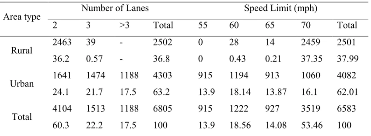
4 Number and percentage of observations within area types, by number of lanes and speed limit ... 36
5 List of the dummy variables considered for the analysis ... 38
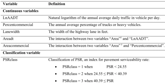
6 List of the continuous and classification variables considered for the analysis ... 39
7 NB model estimates ... 42
8 Analysis of statistical significance of the effect of change in the number of lanes and speed limit on crash frequency ... 45
9 Statistical significance of the effect of change in the number of lanes and speed limit in the model estimated by the method of maximum likelihood estimation ... 46
10 Comparison of relatively smaller χ2-values ... 48
11 Negative binomial model estimates using generalized estimating equations for three different analysis periods ... 50
Paper III 1 Definition of the continuous and dummy variables considered for analysis ... 67
2 Definition of the interaction variables considered for analysis ... 68
3 Negative binomial model parameter estimates ... 70
4 Overall amount and statistical significance of the effect of change in the number of lanes and speed limit on crash frequency in urban areas of Missouri ... 75
5 Amount and statistical significance of the effect of change in the number of lanes and speed limit on crash frequency in urban areas during the winter season ... 78
SECTION
1. INTRODUCTION
Traffic safety in transportation networks is one of the main priorities for many government agencies, private organizations and the society as a whole. This is mainly due to the significant monetary and non-monetary costs associated with crashes (Elvik, 2000). According to the National Highway Traffic Safety Administration, 5,505,000 traffic crashes occurred in 2009 on the US highways in which 33,808 people died and 2,217,000 people were injured (NHTSA, 2009). Peden et al. (2004) found that the trend in road related injuries are expected to increase from ranked ninth in 1990 to the third largest contributor to the global burden of disease and injury in 2020. This immense loss to society resulting from motor vehicle crashes warrants careful crash evaluation and safety analysis to accurately identify crash contributing factors and countermeasures. HSM (2010) regards crash frequency as a fundamental indicator of “safety” in terms of evaluation and estimation.
Crash analysis research in general has focused on the estimation of traditional crash prediction models such as negative binomial (NB) and Poisson regression models and their generalized forms due to their relatively good fit to the data (Shankar et al., 1995; Poch and Mannering, 1996; Abdel-Aty and Radwan, 2000; Savolainen and Tarko, 2005; Mojtaba Ale Mohammadi et al., 2014a). These crash prediction models have also been used for crash evaluation purposes. HSM (2010) refers to the term “crash
evaluation” as the process of determining the effectiveness of a particular treatment after its implementation. Many studies have been conducted to investigate the effect of
improvement programs on facilities such as rail-highway grade crossings (Hauer and Persaud, 1987), highway segments (Zegeer and Deacon, 1987; Squires and Parsonson, 1989; Knuiman et al., 1993), and intersections (Poch and Mannering, 1996; Datta et al., 2000). One of the issues that has been raised regarding the use of these traditional models on “crash evaluation” is the statistical phenomenon of regression to the mean that occurs when the same unit of observations is repeatedly measured over time (Barnett et al.,
2005). This phenomenon may result in biased estimates in any such investigations and mask the real effectiveness of any countermeasure which in turn clouds the judgment of the evaluators and results in unwise decisions. Empirical Bayes (EB) method has also been used for before-after studies to evaluate the effect of countermeasures on safety, which properly accounts for the regression to the mean while normalizing for differences in traffic volume and other factors between the before and after periods (Hauer, 1997; Persaud et al., 2004; Guo et al., 2010b; Shively et al., 2010; Yu et al., 2013b). But EB method is a relatively sophisticated method that requires extensive data and considerable training and experience (Persaud and Lyon, 2007).
This study presents a simple new approach to addresses the problems mentioned above. A traditional negative binomial regression model was developed using the introduced method to examine the effect of implementation of the Missouri Strategic Highway Safety Plan (MSHSP). The MSHSP data was chosen as it provides an excellent situation of safety improvement intervention on the highways of Missouri. In addition it and evaluate the effects of MSHSP on the crash frequency of various collision types and severity levels. The negative binomial regression models were developed to account for the before-through-change conditions using a continuous variable that is set to zero for pre-implementation years and gradually increases over the implementation years to reach a plateau at the conclusion of the plans.
In the second section of this study, a (longitudinal) negative binomial model was developed using ten years of data (2002-2011). Lord and Persaud (2000) suggest that more years of data adds up to the reliability of the model estimates by reducing the standard errors in the prediction models mentioned above; However, when many years of data is considered the serial correlation in the repeated observations violates the
independence assumptions on unobserved error terms in traditional Poisson and/or NB crash frequency models. This violation creates biased and inefficient models by
underestimating the standard errors. Researchers have tried to use different techniques to account for these temporal correlations between the repeated crash frequencies observed for a highway segment over the years. Examples of the utilized methodologies can be found in Maher and Summersgill (1996) using an iterative solution based on the method of “constructed variables” presented by McCullagh and Nelder (1989), in Ulfarsson and
Shankar (2003) using negative multinomial (NM) models, in Dong, Richards, et al. (2014) using multivariate random parameter models, and in Venkataraman et al. (2014) using random parameter negative binomial models. These methodologies, however, have shown to be not practically applicable for different situations. For example, the analyst need to know the extent and type of correlation prior to the analysis that is not always known (Lord and Persaud, 2000), or the estimation methodology for multivariate random parameter models – the full Bayesian method – is complex and requires training and practice. The implementation and transferability of the method is also a challenge. Wang and Abdel-Aty (2006) used generalized estimating equations (GEE) technique to account for these correlations in a frequency model for rear-end crashes at signalized
intersections. This technique has the potential of addressing the issue of serial
correlations in the repeated observations, producing reasonably accurate standard errors and efficient parameter estimates (Méndez et al., 2010; Peng et al., 2012; Giuffrè et al., 2013; Stavrinos et al., 2013). Liang and Zeger (1986) were the first to use this technique to model repeated observations and showed that the GEE method is robust to
misspecification of the correlation structure but Giuffrè et al. (2007) and Ballinger (2004) demonstrated that utilizing the true data correlation structure in safety modeling results in higher estimation precision. In spite of all this research on the effects of temporal
correlations in crash data, consequences arising from the omission of the serial correlation are still not completely understood.
The longitudinal negative binomial model developed in the second part of this study presents an application of the GEE method to model several years of crash frequency data in Missouri. This analysis first determines the temporal correlation structure in the data, proceeds with the analysis, and finally validates the correlation structure used in the analysis as an appropriate structure in this type of data. During the analysis, several data-related obstacles had to be addressed including the
multicollinearity, sufficiency of the within-cluster observations, and the confounding effects. Interaction of the major crash contributing factors with the area type was also examined to evaluate whether crash causes behave differently from rural to urban areas. The results of this model were then compared with a traditional NB model using the
chi-square values of the estimated model parameters and the cumulative residual (CURE) plots. Details of this part of the study are presented in the section “Paper II”.
The results of the second section provide a better understanding of the true factors that affect the occurrence of crashes. The third part of this study is also involved in improvements of the crash evaluation model. Crashes are usually caused by several factors related to drivers’ behavior, vehicles, highway design, and environmental conditions. Geographic location and the climatic environment, particularly seasonal weather can be a major factor that contributes to the occurrence of crashes (Garber and Hoel, 2008b). There are few studies in the crash evaluation realm dealing with the seasonal effects of crashes, but to the best knowledge of the author, no in-depth analysis of the seasonality of crash causes has been conducted. Some examples of the previous studies on the seasonality effects include the works of Carson and Mannering (2001), Hilton et al. (2011), Ahmed et al. (2011), Yu et al. (2013a), and Yang et al. (2013) that have shown that with a better understanding of the crash causes over different times of the year, policy-makers can improve the safety of specific roadway segments according to the seasonal weather patterns and that different traffic management strategies should be designed based on seasons.
The objective of the analysis in the third paper is to further investigate the
seasonal effects on crash causality factors by developing a longitudinal negative binomial model using ten years of crash data on six main interstate highways of Missouri. This analysis uses generalized estimating equation (GEE) technique to develop the model. The interaction of the main variables with the seasonal indicators were examined in the model to gain a better understanding of the change in the effect of crash causes over different seasons in a year. The effects of interventions made by the Missouri Strategic Highway Safety Plan (MSHSP) over the years 2005-2011 is also investigated. The detailed results of this analysis (presented in the section “Paper III”) can help in developing policies regarding highway safety countermeasures with insight on the effects of seasonal changes on roadway fatality factors.
PAPER
I. SAFETY EFFECT OF MISSOURI’S STRATEGIC HIGHWAY SAFETY PLAN - MISSOURI’S BLUEPRINT FOR SAFER ROADWAYS
ABSTRACT
This study systematically evaluates the changes in motor vehicle crashes that occurred on the Missouri interstate highway system following the implementation of Missouri’s Strategic Highway Safety Plan (MSHSP) between 2004 and 2007. The MSHSP implemented crash injury reduction strategies in enforcement, education, engineering, and public policy. Empirical Bayesian methods are commonly used to evaluate the effects of any change in safety as a result of countermeasures. This study presents a simple new approach to evaluating the effects of Missouri’s safety plans on roadway crashes. For crash data associated with traffic and roadway characteristics, negative binomial regression models were developed for the before-through-change conditions using a variable that is set to zero for pre-implementation years and gradually increases over the implementation years to reach a plateau at the conclusion of the safety plans. The models developed for the various collision types and crash severities were used to estimate the expected number of crashes at roadway segments in 2008, assuming with and without the implementation of MSHSP. This procedure estimated significant reductions of 10% in the overall number of crashes and a 30% reduction for fatal crashes. Reductions in the number of different collision types were estimated to be 18-37%. The theoretical results indicate that the MSHSP was a successful policy in reducing the number of crashes and decreasing fatalities by reducing the most severe collision types like head-on crashes. The results are also consistent with many international studies and suggest that the safety strategic plans should be promoted as an effective treatment for highways.
Keywords: negative binomial, before-after study, Missouri blueprint, strategic highway safety plan, MSHSP
1. INTRODUCTION
In 2004, a partnership of Missouri safety advocates, including law enforcement agencies, health care providers, government agencies, and others formed the Missouri Coalition for Roadway Safety (MCRS). This group worked with regional safety coalitions to implement the first strategic highway safety plan, titled Missouri’s Blueprint for Safer Roadways. The potentially life-saving and injury reduction strategies in Missouri’s Blueprint were crucial in the areas of education, enforcement, engineering, and public policy. Some of these strategies included the increase in public education and information on traffic safety, expanding roadway shoulders, installation of centerline and shoulder rumble strips, and roadway visibility features such as pavement markings, signs, lighting, etc., removing fixed objects along roadside right of way, and improving curve recognition through the use of signs, markings, and pavement treatments.
The primary emphasis area of the program aimed to reduce the number and severity of serious crash types with a specific focus on run-off-road crashes, crashes involving horizontal curves, head-on crashes, collisions with trees or poles, and intersection crashes (1). The long-range goal of the program was to reach 1000 or fewer fatalities by 2008 which was achieved a year early, when the total number of fatalities was reduced to 992 in 2007. Between 2005 and 2007, the death rate per 100 million vehicle miles of travel dropped from 1.8 to 1.4 and 21% fewer lives were lost on Missouri highways (2). These safety improvements resulted from the implementation of the MSHSP (1, 2). The present study theoretically examines the effect of implementation of the Missouri’s Blueprint for Safer Roadways on the nature and magnitude of crash frequency of various collision types and their severity. The next section presents a review of the previous studies in the literature of highway safety. The paper then describes the approach used in this study along with an introduction to the data set used. The results of the study and the conclusions follow in the next sections.
2. BACKGROUND
Highway safety analysts use regression models for purposes such as establishing relationships between motor vehicle crashes and incorporating factors such as traffic and geometric characteristics of the roadway, predicting values or screening variables (3). Lord and Mannering (4) have documented a considerable amount of research work devoted to the development and application of new and innovative models for analyzing count data. According to Zou et al. (5), due to the over-dispersion in crash data, the negative binomial (NB) model is probably the most frequently used statistical model in various types of highway safety studies for developing crash prediction models. Shankar et al. (6) conducted a negative binomial multivariate analysis of roadway geometrics and weather-related effects. Their work presents a basis for a comprehensive before-and-after analysis of the effectiveness of safety improvements.
Developing quantitative relations to relate various safety improvement plans to crash rates and severities provides the information required to choose between the cost and the benefit of better transportation networks, and also helps in prioritizing the safety improvement projects. Many studies have been conducted in the past decades investigating the effect of improvement programs on facilities such as rail-highway grade crossings (7), highway segments (8-10), and intersections (11, 12).
Researchers have also used the Empirical Bayes (EB) method (13) for conducting observational before-after studies to evaluate the effect of engineering countermeasures on safety. This procedure is often used to properly account for the regression to the mean while normalizing for differences in traffic volume and other factors between the before and after periods. Persaud et al. (14) used the EB procedure to examine the reduction of opposing direction crashes after installation of rumble strips along the centerlines of undivided rural two-lane roads. Bayesian inference methods have also been used in many recent studies to predict crash occurrences (15, 16). Miaou et al. (17) and Ahmed et al. (18) employed the Hierarchical Bayes model to estimate traffic crashes. Shively et al. (19) employed a Bayesian nonparametric estimation procedure in their study. Huang and Abdel-Aty (20) also proposed a hierarchical structure to deal with multilevel traffic safety data. Persaud and Lyon (21) conducted extensive research on the EB methodology and its
statistical application in before-after studies. According to them, there is a need to evaluate the safety effect of roadway improvements that may impact crash frequency, and the EB methodology produces valid results that are substantially different than those produced by more traditional methods. What requires exploration is whether or not it is worth the effort of using a sophisticated methodology such as the EB method in which (a) the relative complexity of the methodology requires analysts with considerable training and experience, and (b) the data needs can be extensive (21).
The more conventional alternatives to the EB method, involving a simple before– after comparison of crash counts or rates, with or without a comparison or control group, are appealing in that they are relatively easy to apply. These alternative methods, however, are loaded with challenges (21): the comparison group needs to be similar to the treatment group in all of the possible factors that could influence safety, and the assumption that the comparison group is unaffected by the treatment is difficult to test and can be unreasonable in some situations.
This study presents a simple new approach to evaluate the effects of MSHSP on Missouri Interstate highway crashes. Using six years of data, including the safety program implementation years (2005 through 2007), negative binomial crash frequency models were developed for predicting the crash frequency for 2008. The prediction models are developed in a way that will address the regression to the mean concern that prevails in such models. The predicted crash frequency with and without the improvements was compared statistically to determine the effect of MSHSP. The models represent a mix of urban and rural environments and were developed for various collision types and crash severities to investigate the safety improvements by estimating the expected number of crashes under different scenarios.
3. METHODOLOGY
The safety of an improved segment of the roadway in general should be estimated by mixing information of causal factors such as traffic flow, type of traffic control devices, geometric properties, etc. (7). The objective of this study is to develop statistical models of the crash frequency for all the interstate highways of Missouri. This study
estimates six different crash frequency models that will predict (1) total crash frequency (all crash types), (2) head-on crash frequency, (3) rear-end crash frequency, (4) sideswipe-same direction crash frequency, (5) sideswipe-opposite direction crash frequency, and (6) angle crash frequency. Additionally, two separate models are developed for the only fatal and only non-fatal crashes. The dependent variable in all models is the crash count with a discrete non-negative integer nature, and Poisson regression is the first natural choice for modeling such data (22-25); however, a major limitation of the Poisson model is that it constrains the variance of dependent variables to be equal to its mean. When the variance of the data is not equal to the mean (which is usually the case in most of the crash frequency data), the variance of the model coefficients tend to be underestimated, which results in biased estimates. Negative binomial models have been extensively used in literature to overcome this limitation by relaxing the condition of ‘variance = mean’ in standard Poisson models (5).
If the length of segment ‘i’ (Li) and the crash observation time interval for segment ‘i’ (ti) for various segments are different, the observed number of crashes on the segment ‘i’ is proportional to the Li and ti. Length and duration of the observation are commonly called to be offset variables as their coefficients are restricted to be one and not estimated (26). In this study, since all the segments are measured over one year, the only offset variable used was the segment length. To describe the formulation of the negative binomial model, the Poisson model for crash counts is first reviewed; according to the Poisson distribution the probability of ‘n’ crashes occurring on segment ‘i’ during time period ‘j’ is:
=
! (1)
Where is the expected number of crashes on segment ‘i’ during time interval ‘j’. Given the vector of incorporating factors, can be estimated by the equation:
ln = (2)
An additional stochastic component ‘ɛ’ is introduced to the link function by assuming ‘eɛ’ Gamma distributed (with mean ‘ ’ and variance ‘ ’) resulting in the Poisson-Gamma model (also called the negative binomial model, NB) (6, 24, 27, 28):
ln = + (3)
An additional parameter ‘ ’ allows the variance to differ from the mean and will result in the following mean-variance relationship:
= 1 + = (1 + ) (4)
If ‘ ’ is equal to zero, the negative binomial reduces to Poisson, and if it is significantly different from zero, the data is either over-dispersed or under-dispersed. Using the Poisson distribution for crash count modeling, the probability of n crashes occurring on segment ‘i’ during time period ‘j’ is:
=Γ +
Γ(θ)n ! + + (5)
Where = 1/ , and Γ(. ) is a value of gamma function. can be estimated using the maximum likelihood estimation (MLE) procedure. The likelihood function for the negative binomial model is:
= Γ +
Γ(θ)n ! + + (6)
Where ‘T’ is the last time interval of the crash count data and ‘N’ is the number of roadway segments. Maximizing this function results in the estimation of ‘ ’ and ‘ ’ (in equations 2 and 3). Using a variable that is set to zero for pre-implementation years and gradually increases over the implementation years (2005 through 2007) to reach a plateau of one at the conclusion of the safety plans and the crash data associated with traffic and roadway characteristics, negative binomial regression models were developed for the before-through-change conditions.
The reduction in the crash frequency after the implementation of the safety plans relative to the frequency values prior to this implementation could be attributed to the simple phenomenon of regression to the mean. If the reduction in the crash frequencies was detected using a model that uses before and after values, then associating this reduction with the implementation of the safety measures may be misleading. Our approach, however, did not merely look at before and after figures or model the change using a dummy variable, but instead utilized a continuous variable named “transition” in the NB model of the analysis to account for the plan implementation through the years. This variable was assigned the value of zero prior to the commencement of the improvements and gradually increased from zero to one, exactly over the implementation period in such a way that its value coincided, approximately, with the proportion of safety features that were completed at a given time. For the years after the completion of the improvements, this variable was kept constant at 1.0, suggesting 100% implementation. The plan included actions such as widening roadway shoulders, installation of centerline and shoulder rumble strips, etc. This study is an attempt to statistically examine the effects of the MSHSP implementation. The transition variable turned out to be highly significant with a negative sign for its coefficient estimate, indicating a close correlation between the reduction in crash frequency and the rate of completion of the safety features. Hence, the likelihood that this reduction reflects a regression to the mean is very low.
4. DATA ANALYZED
The Missouri Department of Transportation (MoDOT) portal of safety investigation provided access to the crash data base for all the recorded years of data. The crash data consists of all severity types of motor-vehicle crashes (fatal, disabling injury, minor injury, and property damage only crashes) at 17 interstate highways in the state of Missouri from 2002 to 2007. Some of the major characteristics of the highways are presented in Table 1. These highways, with an overall length of about 1200 miles, were classified as divided highways located either in urban or rural areas (65% in rural areas and 35% in urban areas). The total number of crashes in the data set analyzed was
167,783 crashes, out of which 37% occurred in rural areas and 63% in urban areas. The rate of crash (number of crashes per mile and number of crashes per vehicle) for a segment in each year is shown in column 2 of the table along with the total number of crashes on all interstate highways presented in column 3.
Table 1. Descriptive statistics of segment properties of interstate highways in Missouri
Year Crash/mile, Crash/1000 car* (min-max) Total number of crashes AADT (min-max) Number of lanes (min-max) PSR (min-max) Percent commercial (min-max) 2002 0-241 , 0-4 18955 1985-101594 1-7 19.3-66.4 0.041-0.582** 2003 0-293 , 0-4 19581 1867-98485 1-7 17.4-37.4 0.041-0.406 2004 0-293 , 0-4 19343 1919-109420 1-6 18.9-37.3 0.046-0.582 2005 0-328 , 0-4 19101 1865-109573 2-6 24-39.6 0.045-0.582 2006 0-500 , 0-3 18922 1874-114753 1-6 23.4-37.5 0.049-0.582 2007 0-333 , 0-4 19308 1893-115901 1-6 22.9-37.6 0.049-0.622
* Minimum rate for all the segments during each year was zero
** This high value of truck percentage probably represents the night time at specific sections of the highways with low traffic
The explanatory variables used in this analysis are number of lanes, lane width (min. 10 ft to max. 18 ft), shoulder width (min. 3 ft to max. 12 ft), average annual daily traffic (AADT), speed limit, congestion index, pavement serviceability rate (PSR), and truck percentage. Other factors such as weather information, roadway conditions, and drivers’ characteristics could not be aggregated for the entire state and yearly level for analysis. PSR is equal to two times the ride number plus the pavement condition index. Ride number is an index derived from controlled measurements of longitudinal profile in the wheel tracks and correlated with rideability of a pavement using a scale of 0 to 5, with 5 being perfect and 0 being impassable. Pavement condition index is a numerical rating of the pavement condition that ranges from 0 to 100 with 0 being the worst possible condition and 100 being the best possible condition. More information on the indices of ride number and pavement condition index can be found on the standards ASTM D6433-07 (29) and ASTM E1489-08 (30) respectively. The higher the value of PSR, the higher the pavement serviceability. Congestion index presents the level of congestion. It is
calculated by incorporating the level of service of the roadway, AADT, and number of lanes. A higher value of congestion index indicates a higher level of congestion.
Variables selected for model development depended on the quality of the data provided, the purpose of the variables, and the significance of those variables in calculating the crash count. More than 6000 segments with an average length of 2.2 miles were identified over the six years of roadway data. MoDOT chose the beginning and ending points of the segments based on the geometric and traffic properties of the segments and were included in roadway segments database.
When a regressor is nearly a linear combination of other regressors in the model, the affected estimates are unstable and have high standard errors. This problem is called collinearity or multicollinearity (31). It is a good idea to find out which variables are nearly collinear with which other variables and remove them from the analysis. Two variables, “congestion index rate” and “pavement index,” in the initial dataset were highly multicollinear with “congestion index” and “PSR” respectively. They were removed from the analysis. A multicollinearity diagnostic was conducted in SAS using PROC REG with the options COLLIN (32). Belsley et al. (31) suggest that in the results of collinearity diagnostics, when the value of ‘condition index’ is larger than 100, the estimates might have a fair amount of numerical error. The values of ‘condition index’ were found as 161.08 and 5210.034 for “pavement index” and ““congestion index rate” respectively.
5. RESULTS
Generalized linear model was used to model the crash counts on the Missouri interstate highway segments using a negative binomial link function. A summary of the parameter estimates and their standard errors for the NB models developed in this study are presented in Table 2. The results indicate that for almost all of the models the variables lane, width, shoulder width, and PSR were not statistically significant factors in crash occurrences.
The signs of the parameter estimates make sense: number of lanes has a negative sign for all models, indicating that higher number of travel lanes reduces the number of
crashes. This is in contrast with some of the previous studies that found higher number of lanes associated with higher risk of crashes (33-36). They used both AADT/n, where n = number of lanes, and n in their studies. We used AADT and n. So, in our study, the coefficient of n stands for the effect of increasing the number of lanes while holding AADT constant for that segment. In other studies ( e.g. Abdel-Aty and Radwan (33) and Milton and Mannering (36)), increasing n means increasing the total AADT for the segment. Therefore, the negative sign of the coefficient of n in our study implies that increasing the number of lanes while keeping AADT constant enhances safely. In other studies, increasing n implies that not only are we increasing the number of lanes, but we are also increasing the amount of traffic. Hence, the positive sign of the coefficient makes sense for these other studies. The natural logarithm of AADT has a positive sign for all models, which indicates a higher number of crashes with higher traffic volume.
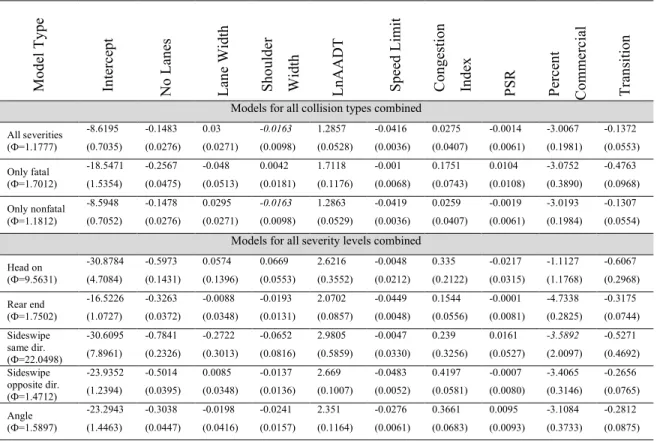
Table 2. Parameter estimates and their standard errors for the different negative binomial models Mo d el T y p e In terc ep t No L an es Lan e Width Sho u lde r Width Ln AADT Spe ed L imit Con g estion In d ex PSR Perc en t Com me rc ial Tr an siti on
Models for all collision types combined All severities (Ф=1.1777) -8.6195 (0.7035) -0.1483 (0.0276) 0.03 (0.0271) -0.0163 (0.0098) 1.2857 (0.0528) -0.0416 (0.0036) 0.0275 (0.0407) -0.0014 (0.0061) -3.0067 (0.1981) -0.1372 (0.0553) Only fatal (Ф=1.7012) -18.5471 (1.5354) -0.2567 (0.0475) -0.048 (0.0513) 0.0042 (0.0181) 1.7118 (0.1176) -0.001 (0.0068) 0.1751 (0.0743) 0.0104 (0.0108) -3.0752 (0.3890) -0.4763 (0.0968) Only nonfatal (Ф=1.1812) -8.5948 (0.7052) -0.1478 (0.0276) 0.0295 (0.0271) -0.0163 (0.0098) 1.2863 (0.0529) -0.0419 (0.0036) 0.0259 (0.0407) -0.0019 (0.0061) -3.0193 (0.1984) -0.1307 (0.0554) Models for all severity levels combined
Head on (Ф=9.5631) -30.8784 (4.7084) -0.5973 (0.1431) 0.0574 (0.1396) 0.0669 (0.0553) 2.6216 (0.3552) -0.0048 (0.0212) 0.335 (0.2122) -0.0217 (0.0315) -1.1127 (1.1768) -0.6067 (0.2968) Rear end (Ф=1.7502) -16.5226 (1.0727) -0.3263 (0.0372) -0.0088 (0.0348) -0.0193 (0.0131) 2.0702 (0.0857) -0.0449 (0.0048) 0.1544 (0.0556) -0.0001 (0.0081) -4.7338 (0.2825) -0.3175 (0.0744) Sideswipe same dir. (Ф=22.0498) -30.6095 (7.8961) -0.7841 (0.2326) -0.2722 (0.3013) -0.0652 (0.0816) 2.9805 (0.5859) -0.0047 (0.0330) 0.239 (0.3256) 0.0161 (0.0527) -3.5892 (2.0097) -0.5271 (0.4692) Sideswipe opposite dir. (Ф=1.4712) -23.9352 (1.2394) -0.5014 (0.0395) 0.0085 (0.0348) -0.0137 (0.0136) 2.669 (0.1007) -0.0483 (0.0052) 0.4197 (0.0581) -0.0007 (0.0080) -3.4065 (0.3146) -0.2656 (0.0765) Angle (Ф=1.5897) -23.2943 (1.4463) -0.3038 (0.0447) -0.0198 (0.0416) -0.0241 (0.0157) 2.351 (0.1164) -0.0276 (0.0061) 0.3661 (0.0683) 0.0095 (0.0093) -3.1084 (0.3733) -0.2812 (0.0875) - Bold numbers indicate significance at 95% confidence level, and italic numbers at 90% confidence level.
Speed limit has a negative sign for all the models developed; indicating higher speed limits decrease the number of crashes. The sign can be explained as: these models do not indicate if the crash happened in an urban or rural area; it is therefore reasonable to state that fewer crashes occur in the rural areas as a result of lesser traffic, and rural areas have higher speed limit. The speed limit is another way to capture the changes in the number of crashes as a result of a change in type of area. The congestion index was also found to have a positive sign on models where it is a significant factor. This indicates that a higher number of crashes occur with more congestion, which is very similar to AADT. Percent commercial has a negative sign and was found to be significant, which indicates that higher percentage of heavy vehicles in the traffic mix results in fewer crashes. This indicates that drivers in general take caution around heavy vehicles. It was also found that the percentage of heavy vehicles had the highest effect on the reduction of rear-end crashes.
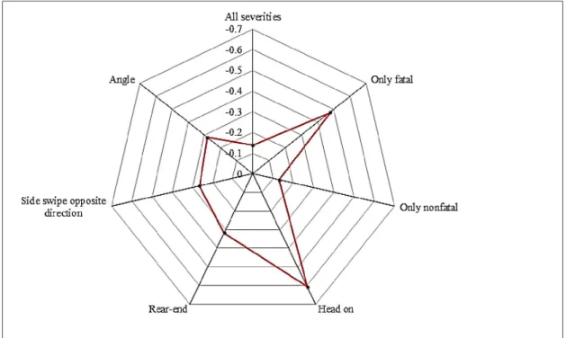
The transition variable was designated in the model to capture the effects of the safety strategies during the years 2005 through 2007. This factor was found to be statistically significant at 95% level of confidence and have a negative sign on all the models developed. The negative sign of the estimate indicates a reduction in the number of crashes during the implementation years, 2005 - 2007. The estimated values for this parameter indicates that the safety improvement strategies were mostly effective in reducing the fatal crashes compared to nonfatal crashes and in reducing the head-on crashes (leading cause of fatal crashes), compared to the other types of collisions (see the spider chart in Figure 1). The effect on crash type sideswipe-same direction is not shown in the figure as it was not found to be significant. A clear connection between the two findings can be observed from Figure 1; head-on collisions are the most severe types of crashes that result in fatalities.
The transition variable was used with four continuous quantitative levels from 0 before 2005, and then 0.25 to 0.75 from 2005 to 2007 for each year. It was used to investigate the predicted values of crashes in 2008, assuming with/without safety improvements, and the predicted numbers for different models were compared. shows the mean, standard deviation, min, max, and sum of the predicted crash counts in an interstate roadway segment for the year 2008, assuming there were/were not safety
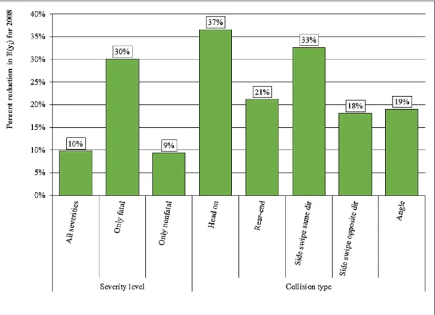
improvements implemented on the interstate highways. Comparing the “without” condition with the “with” condition, a drop can be observed in all the measures shown in Figure 2 presents a clear illustration of the percent reduction in the expected value of the number of crashes for 2008 as a result of the safety improvement program. It can be observed that the highest reduction (highest safety improvement effect) was 30% for only-fatal crashes. In terms of the collision type, the safety enhancement strategies had the highest effect on head-on crashes. This type of crash specifically results in high fatalities and the goal of the MSHSP was to reduce the number of fatal crashes. It was also found that the highway safety improvements result in a reduction of 18-33% in the number of other collision types including rear-end, sideswipe same- and opposite-direction, and angle crashes.
Figure 1. Graphical comparison of the effect of safety improvements on the crash models developed (values represent the estimate for the transition variable for each model).
Table 3, indicating the safety enhancing effects of the Missouri Blueprint
strategies. It can also be observed that the maximum number of crashes included rear-end and sideswipe-same direction crashes. Figure 2 presents a clear illustration of the percent reduction in the expected value of the number of crashes for 2008 as a result of the safety improvement program. It can be observed that the highest reduction (highest safety
improvement effect) was 30% for only-fatal crashes. In terms of the collision type, the safety enhancement strategies had the highest effect on head-on crashes. This type of crash specifically results in high fatalities and the goal of the MSHSP was to reduce the number of fatal crashes. It was also found that the highway safety improvements result in a reduction of 18-33% in the number of other collision types including rear-end,
sideswipe same- and opposite-direction, and angle crashes.
Table 3. Comparison of the predicted crash count properties for 2008 with/without safety improvements Model Type Mean with o u t * Mean with * Std ev w ith o u t Std ev w ith Min w ithout Min w ith Max wi th out Max wi th Sum wi th out Sum wi th
Models for all collision types combined
All severities 9.590 8.652 23.186 20.919 0.04815 0.04344 188.175 169.774 10453.12 9430.98
Only fatal 0.148 0.103 0.163 0.114 0.00083 0.00058 0.986 0.689 161.35 112.88
Only nonfatal 9.576 8.682 23.317 21.139 0.04706 0.04266 189.527 171.830 10438.02 9463.39
Models for all severity levels combined
Head on 0.011 0.007 0.017 0.011 9.46E-06 6.00E-06 0.168 0.106 12.90 8.18 Rear end 5.668 4.467 16.520 13.020 0.001695 0.001335 183.230 144.405 6178.20 4869.07 Sideswipe
same dir. 0.005 0.003 0.009 0.006 7.56E-07 5.09E-07 0.100 0.067 5.96 4.01 Sideswipe
opp. dir. 2.325 1.905 7.629 6.251 0.000216 0.000177 114.669 93.958 2535.22 2077.33 Angle 0.445 0.361 0.949 0.768 0.00021 0.00017 10.942 8.861 486.10 393.67 * “without” and “with” indicates that model estimates for 2008 are determined assuming without and with safety improvements respectively
Figure 2. Percent reduction in the expected number of crashes predicted in 2008 as a result of safety improvement strategies.
6. CONCLUSIONS AND RECOMMENDATIONS
The objective of this study was to use a simple new approach to evaluate the effects of Missouri’s Strategic Highway Safety Plan (MSHSP) on the number of crashes that occurred on the Missouri Interstate highways. Through the years 2004 to 2007, the MSHSP was implemented in enforcement, education, engineering, and public policy. Using a continuous variable through the implementation years, negative binomial regression models were developed and used to estimate the expected number of crashes in 2008 with and without the implementation of MSHSP. The results show that this safety enhancement program was able to reach its primary goal, i.e. to reduce the number and severity of serious injury crash types.
The study found a significant reduction of 10% for all crash severities combined and 30% for only fatal crashes. These strategies had the highest effect on the fatal crashes and particularly on the head-on crashes that result the most fatalities (1, 2). It was also
found that the highway safety improvements result in a reduction of 18-37% in the number of different collision types. The results from the model indicate that the MSHSP was a successful policy in reducing the overall number of crashes and decreasing the fatalities by decreasing the most severe injury crash types. The results are also consistent with many international studies and suggest that the safety strategic plans should be promoted as an effective treatment for highway crash fatalities (37, 38). However, further analysis of particular SHSP implementation effectiveness that focus on the specific emphasis areas identified in the SHSP is warranted in future studies to obtain a more detailed understanding of how the implementation of specific safety measures affect safety. Provided the specific implementation data on the highways are available, future studies will consider examination of the effect of safety improvement plans (such as ‘adding median barrier’) on the type and injury severity of crashes.
7. REFERENCES
1. MoDOT. Missouri's blueprint for safer roadways. 2004 http://www.ite.org/safety/stateprograms/Missouri_SHSP.pdf. Accessed Nov. 10, 2013.
2. MoDOT. Missouri's blueprint to arrive alive. 2008 http://www.savemolives.com/documents/FINALBlueprintdocument.pdf.
Accessed Nov. 10, 2013.
3. Geedipally, S.R., D. Lord, and S.S. Dhavala, The negative binomial-Lindley generalized linear model: Characteristics and application using crash data. Accident Analysis & Prevention, 2012. 45: p. 258-265.
4. Lord, D. and F. Mannering, The statistical analysis of crash-frequency data: A review and assessment of methodological alternatives. Transportation Research Part A: Policy and Practice, 2010. 44(5): p. 291-305.
5. Zou, Y., et al. Comparison of Sichel and Negative Binomial Models in Estimating Empirical Bayes Estimates. in Transportation Research Board 92nd Annual Meeting. 2013.
6. Shankar, V.N., F. Mannering, and W. Barfield, Effect of roadway geometrics and environmental factors on rural freeway accident frequencies. Accident Analysis & Prevention, 1995. 27(3): p. 371-389.
7. Hauer, E. and B. Persaud, How to estimate the safety of rail-highway grade crossings and the safety effects of warning devices1987: Transportation Research Board.
8. Knuiman, M.W., F.M. Council, and D.W. Reinfurt, Association of median width and highway accident rates. Transportation Research Record, 1993: p. 70-70.
9. Squires, C.A. and P.S. Parsonson, Accident comparison of raised median and two-way left-turn lane median treatments. Transportation Research Record, 1989. 1239: p. 30-40.
10. Zegeer, C.V. and J.A. Deacon, Effect of lane width, shoulder width, and shoulder type on highway safety. State-of-the-Art Report, 1987(6).
11. Poch, M. and F. Mannering, Negative binomial analysis of intersection-accident frequencies. Journal of transportation engineering, 1996. 122(2): p. 105-113. 12. Datta, T.K., K. Schattler, and S. Datta, Red light violations and crashes at urban
intersections. Transportation Research Record: Journal of the Transportation Research Board, 2000. 1734(1): p. 52-58.
13. Hauer, E., Observational Before/After Studies in Road Safety. Estimating the Effect of Highway and Traffic Engineering Measures on Road Safety1997.
14. Persaud, B., R.A. Retting, and C.A. Lyon, Crash reduction following installation of centerline rumble strips on rural two-lane roads. Accident Analysis & Prevention, 2004. 36(6): p. 1073-1079.
15. Yu, R., M. Abdel-Aty, and M. Ahmed, Bayesian random effect models incorporating real-time weather and traffic data to investigate mountainous freeway hazardous factors. Accident Analysis & Prevention, 2013. 50: p. 371-376.
16. Guo, F., X. Wang, and M.A. Abdel-Aty, Modeling signalized intersection safety with corridor-level spatial correlations. Accident Analysis & Prevention, 2010. 42(1): p. 84-92.
17. Miaou, S.-P., J.J. Song, and B.K. Mallick, Roadway traffic crash mapping: A space-time modeling approach. Journal of Transportation and Statistics, 2003. 6: p. 33-58.
18. Ahmed, M., et al., Exploring a Bayesian hierarchical approach for developing safety performance functions for a mountainous freeway. Accident Analysis & Prevention, 2011. 43(4): p. 1581-1589.
19. Shively, T.S., K. Kockelman, and P. Damien, A Bayesian semi-parametric model to estimate relationships between crash counts and roadway characteristics. Transportation research part B: methodological, 2010. 44(5): p. 699-715.
20. Huang, H. and M. Abdel-Aty, Multilevel data and Bayesian analysis in traffic safety. Accident Analysis & Prevention, 2010. 42(6): p. 1556-1565.
21. Persaud, B. and C. Lyon, Empirical Bayes before–after safety studies: lessons learned from two decades of experience and future directions. Accident Analysis & Prevention, 2007. 39(3): p. 546-555.
22. Lord, D., S.P. Washington, and J.N. Ivan, Poisson, Poisson-gamma and zero-inflated regression models of motor vehicle crashes: balancing statistical fit and theory. Accident analysis and prevention, 2005. 37(1): p. 35-46.
23. Jones, B., L. Janssen, and F. Mannering, Analysis of the frequency and duration of freeway accidents in Seattle. Accident Analysis & Prevention, 1991. 23(4): p. 239-255.
24. Miaou, S.-P., The relationship between truck accidents and geometric design of road sections: Poisson versus negative binomial regressions. Accident Analysis & Prevention, 1994. 26(4): p. 471-482.
25. Shankar, V.N., J. Milton, and F. Mannering, Modeling accident frequencies as zero-altered probability processes: an empirical inquiry. Accident Analysis & Prevention, 1997. 29(6): p. 829-837.
26. Uhm, T., M.V. Chitturi, and A.R. Bill. Comparing Statistical Methods for Analyzing Crash Frequencies. in Transportation Research Board 91st Annual Meeting. 2012.
27. Kulmala, R., Safety at rural three- and four-arm junctions: development and applications of accident prediction models., 1995, Technical Research Centre of Finland: Espoo. Finland.
28. Lee, J. and F. Mannering, Impact of roadside features on the frequency and severity of run-off-roadway accidents: an empirical analysis. Accident Analysis & Prevention, 2002. 34(2): p. 149-161.
29. ASTM-D6433-07, Standard Practice for Roads and Parking Lots Pavement Condition Index Surveys, 2007, ASTM International: West Conshohocken, PA. 30. ASTM-E1489-08, Standard Practice for Computing Ride Number of Roads from
Longitudinal Profile Measurements Made by an Inertial Profile Measuring Device, 2008, ASTM International: West Conshohocken, PA.
31. Belsley, D.A., E. Kuh, and R.E. Welsch, Regression diagnostics: Identifying influential data and sources of collinearity. Vol. 571. 2005: John Wiley & Sons. 32. Littell, R.C., W.W. Stroup, and R.J. Freund, SAS for linear models. 2002: SAS
Institute.
33. Abdel-Aty, M.A. and A.E. Radwan, Modeling traffic accident occurrence and involvement. Accident Analysis & Prevention, 2000. 32(5): p. 633-642.
34. Chang, L.-Y., Analysis of freeway accident frequencies: negative binomial regression versus artificial neural network. Safety science, 2005. 43(8): p. 541-557.
35. Noland, R.B. and L. Oh, The effect of infrastructure and demographic change on traffic-related fatalities and crashes: a case study of Illinois county-level data. Accident Analysis & Prevention, 2004. 36(4): p. 525-532.
36. Milton, J.C. and F.L. Mannering, The relationship between highway geometrics, traffic related elements, and motor vehicle accidents. 1996.
37. Jung, S., Q. Xiao, and Y. Yoon, Evaluation of motorcycle safety strategies using the severity of injuries. Accident Analysis & Prevention, 2013. 59: p. 357-364. 38. Kempton, W., et al., California Strategic Highway Safety Plan, Version 2.
California Business, Transportation, Housing Agency Contributing Departments, Sacramento, CA. , 2006.
II. CRASH FREQUENCY MODELING USING NEGATIVE BINOMIAL MODELS: AN APPLICATION OF GENERALIZED ESTIMATING EQUATION
TO LONGITUDINAL DATA
ABSTRACT
The prediction of crash frequency models can be improved when several years of crash data are utilized, instead of three to five years of data most commonly used in research. Crash data, however, generates multiple observations over the years that can be correlated. This temporal correlation affects the estimated coefficients and their variances in commonly used crash frequency models (such as negative binomial (NB), Poisson models, and their generalized forms). Despite the obvious temporal correlation of
crashes, research analyses of such correlation have been limited and the consequences of this omission are not completely known. The objective of this study is to explore the effects of temporal correlation in crash frequency models at the highway segment level.
In this paper, a negative binomial model has been developed using a generalized estimating equation (GEE) procedure that incorporates the temporal correlations amongst yearly crash counts. The longitudinal model employs an autoregressive correlation structure to compare to the more traditional NB model, which uses a Maximum
Likelihood Estimation (MLE) method that cannot accommodate temporal correlations. The GEE model with temporal correlation was found to be superior compared to the MLE model, as it does not underestimate the variance in the coefficient estimates, and it provides more accurate and less biased estimates. Furthermore, an autoregressive
correlation structure was found to be an appropriate structure for longitudinal type of data used in this study. Ten years (2002 - 2011) of Missouri Interstate highway crash data have been utilized in this paper. The crash data comprises of traffic characteristics and geometric properties of highway segments.
Keywords: generalized estimation equation, longitudinal analysis, temporal correlation, crash frequency model, autocorrelation, autoregressive
1. INTRODUCTION
Crash analysis research in general has focused on the estimation of traditional crash prediction models such as negative binomial (NB) and Poisson regression models and their generalized forms due to their relatively good fit to the crash (Shankar et al., 1995; Poch and Mannering, 1996; Abdel-Aty and Radwan, 2000; Savolainen and Tarko, 2005; Mojtaba Ale Mohammadi et al., 2014a). Such crash prediction models take into account the crash frequency of a transportation facility (unit of analysis), such as an intersection or highway segment as a function of traffic flow and other crash-related factors. In these predictions, a greater amount of crash data, i.e. years of data, adds up to the reliability of the model estimates by reducing the standard errors (Lord and Persaud, 2000); However, the same unit generates multiple observations over the years that might be correlated due to unobserved effects related to specific entities that remain constant over time (Park and Lord, 2009; Castro et al., 2012; Bhat et al., 2014; Mannering and Bhat, 2014; Zou et al., 2014). In fact, these unobserved effects create a serial correlation in the repeated observations from the same unit over the years. Serial correlation in longitudinal data is an important issue, as it violates the independence assumptions on unobserved error terms in Poisson and/or NB crash frequency models, and creates inefficiency in the coefficient estimations and bias (underestimation) in estimation of standard error (Ulfarsson and Shankar, 2003; Washington et al., 2011; Dupont et al., 2013; Mohammadi et al., 2013; Bhat et al., 2014; Xiong et al., 2014).
Marginal models appear to be the most appropriate models for handling the temporal correlation, such as the work of Maher and Summersgill (1996) that uses an iterative solution based on the method of “constructed variables” presented by
McCullagh and Nelder (1989). However, the extent and type of temporal correlation requires prior information that is not always known to the analyst (Lord and Persaud, 2000). Ulfarsson and Shankar (2003) tried to address the unit-specific serial correlation issue by using negative multinomial (NM) models in panel data and comparing the results with NB and random-effect negative binomial (RENB) model estimates. They showed that when there is correlation in the segment specific observations, the NM model is a much better fit compared to NB and RENB models. Dong, Richards, et al.
(2014) developed multivariate random parameter models to account for the correlated crash frequency data as a result of unobserved heterogeneity. However, the model estimation methodology –the full Bayesian method– is complex, and the implementation and transferability of the method is not straightforward. Other research studies have been conducted in road safety analysis to account for such correlations in longitudinal data, yet consequences of the omission of the serial correlation are still not completely known. The most recent studies using longitudinal crash data include the work conducted by
Venkataraman et al. (2014) to develop random parameter negative binomial models to investigate heterogeneity in crash means and the effects of interchange type on crash frequency.
Negative binomial models with a trend variable have also been used to study crash data with temporal correlation (Lord and Persaud, 2000; Noland et al., 2008; Quddus, 2008; Chi et al., 2012). Wang and Abdel-Aty (2006) used the technique of generalized estimating equations (GEE) to model rear-end crash frequencies at signalized intersections in order to account for the temporal and/or spatial correlation. GEE treats each highway segment as a cluster whose crash frequency observations have a temporal correlation over multiple years. In statistical terms, GEE captures the correlation
incorporated in the error terms for model estimation. Hanley et al. (2003) showed that the use of GEE has the advantage of producing reasonably accurate standard errors and confidence intervals, especially when there are many subjects and few events. Hutchings et al. (2003) compared the performance of GEE with logistic regression by examining the change in parameter and variance estimates and the statistical significance of the
independent variables. They found a lower number of significant variables when using the GEE method, and so recommended the use of nested structure models and GEE for analyzing motor vehicle crashes. H. L. Chang et al. (2006) applied the GEE procedure in a study of the effectiveness of drivers’ license revocation and its impact on offenders in Taiwan. Lenguerrand et al. (2006) used multilevel logistic models (MLM), GEE, and logistic models (LM) to analyze hierarchical correlated crash data structure and found that both GEE and LM underestimate the parameters and confidence intervals, making MLM the most efficient model followed by GEE and LM models.
Lord and Mahlawat (2009) used GEE method with an autoregressive (AR) correlation structure to investigate the effect of a small sample size and low mean value of crash frequency on the reliability of the inverse dispersion parameter estimate. They found that the standard errors of the models’ coefficients are larger when the serial correlation is accounted for in the modeling process. Méndez et al. (2010) used both logistic regression and GEE models (with exchangeable correlation structure) to study the relationship of a car’s registration year and its crashworthiness. Peng et al. (2012) also utilized the GEE method with an exchangeable correlation structure to study the
relationship between drivers’ inattention and their inability in lane keeping. Stavrinos et al. (2013) used a GEE Poisson regression to study the impact of various distractions on driving behavior. Since the GEE models are not based on maximum likelihood estimation (MLE), they used a Chi-square test to estimate the significance of the variables. Giuffrè et al. (2013) studied the concepts of dispersion and correlation in yearly crash frequency data and presented a quasi-Poisson model in a GEE framework to incorporate both the dispersion and temporal correlation. In comparing the GEE with the COM-Poisson regression model, they recommended the use of GEE whenever it is handy. GEE procedure is robust against misspecification of the correlation structure in the response variable, but in that case, one may lose significant model efficiency and cause a
misleading interpretation of the results, which in turn affects the reliability of the final safety estimation (Giuffrè et al., 2013).
The examples outlined above illustrate how GEE is not actually a regression model, but rather a method used to estimate models for data characterized by serial correlation. Throughout this paper, the models with temporal correlation that use GEE procedure are referred to as the GEE models. Unlike the traditional marginal models, the GEE models can handle temporal or other forms of correlation, even if the extent and type of correlation is unknown. However, Giuffrè et al. (2007) demonstrated that utilizing data correlation structure in safety modeling results in higher estimation precision.
Although they have acknowledged that GEE models generally are robust to
misspecification of the correlation structure (Liang and Zeger, 1986), and researchers believe the true correlation structure is important only when marginal models are estimated by using data with missing values, but when the specified structure does not