Massive Multi-Antenna Communications with Low-Resolution Data Converters

thesis for the degree of doctor of philosophy

Massive Multi-Antenna Communications with

Low-Resolution Data Converters

Sven Jacobsson

Communications, Antennas, and Optical Networks Department of Electrical Engineering

Chalmers University of Technology Gothenburg, Sweden, 2019

Massive Multi-Antenna Communications with Low-Resolution Data Converters

Sven Jacobsson ISBN 978-91-7905-153-2

Copyright © 2019_{Sven Jacobsson}, except where otherwise stated. All rights reserved.

Doktorsavhandlingar vid Chalmers tekniska högskola Ny serie nr 4620

ISSN 0346-718X

This thesis has been prepared using LA_{TEX and TikZ.} Communications, Antennas, and Optical Networks Department of Electrical Engineering

Chalmers University of Technology SE-412 96 Gothenburg, Sweden Phone: +46 (0)31 772 1746 www.chalmers.se

Printed by Chalmers Reproservice Gothenburg, Sweden, August 2019

Abstract

Massive multi-user (MU) multiple-input multiple-output (MIMO) will be a core tech-nology in future cellular communication systems. In massive MU-MIMO systems, the number of antennas at the base station (BS) is scaled up by several orders of magnitude compared to traditional multi-antenna systems with the goals of enabling large gains in capacity and energy efficiency. However, scaling up the number of active antenna elements at the BS will lead to significant increases in power consumption and system costs unless power-efficient and low-cost hardware components are used. In this thesis, we investigate the performance of massive MU-MIMO systems for the case when the BS is equipped with low-resolution data converters.

First, we consider the massive MU-MIMO uplink for the case when the BS uses low-resolution analog-to-digital converters (ADCs) to convert the received signal into the dig-ital domain. Our focus is on the case where neither the transmitter nor the receiver have anya priori channel state information (CSI), which implies that the channel realizations have to be learned through pilot transmission followed by BS-side channel estimation, based on coarsely quantized observations. We derive a low-complexity channel estimator and present lower bounds and closed-form approximations for the information-theoretic rates achievable with the proposed channel estimator together with conventional linear detection algorithms.

Second, we consider the massive MU-MIMO downlink for the case when the BS uses low-resolution digital-to-analog converters (DACs) to generate the transmit signal. We derive lower bounds and closed-form approximations for the achievable rates with linear precoding under the assumption that the BS has access to perfect CSI. We also propose novel nonlinear precoding algorithms that are shown to significantly outperform linear precoding for the extreme case of 1-bit DACs. Specifically, for the case of symbol-rate 1-bit DACs and frequency-flat channels, we develop a multitude of nonlinear precoders that trade between performance and complexity. We then extend the most promising nonlinear precoders to the case of oversampling 1-bit DACs and orthogonal frequency-division multiplexing for operation over frequency-selective channels.

Third, we extend our analysis to take into account other hardware imperfections such as nonlinear amplifiers and local oscillators with phase noise.

The results in this thesis suggest that the resolution of the ADCs and DACs in mas-sive MU-MIMO systems can be reduced significantly compared to what is used in today’s state-of-the-art communication systems, without significantly reducing the overall sys-tem performance.

Keywords: Massive multi-user multiple-input multiple-output, analog-to-digital con-verter, digital-to-analog concon-verter, quantization, hardware impairments, beamforming, channel estimation, linear combing, linear precoding, nonlinear precoding, convex opti-mization, orthogonal frequency-division multiplexing.

List of Publications

This thesis is based on the following publications:

[A] S. Jacobsson, G. Durisi, M. Coldrey, U. Gustavsson, and C. Studer, “Throughput analysis of massive MIMO uplink with low-resolution ADCs”, IEEE Transactions on Wireless Communications, vol. 16, no. 6, pp. 4038–4051, Jun. 2017.

[B] S. Jacobsson, G. Durisi, M. Coldrey, T. Goldstein, and C. Studer, “Quantized pre-coding for massive MU-MIMO,” IEEE Transactions on Communications, vol. 65, no. 11, pp. 4670–4684, Nov. 2017.

[C] S. Jacobsson, W. Xu, G. Durisi, and C. Studer, “MSE-optimal 1-bit precoding for multiuser MIMO via branch and bound,” inProceedings of IEEE International Conference on Acoustics, Speech and Signal Processing (ICASSP), Calgary, AB, Canada, Apr. 2018, pp. 3589–3593.

[D] S. Jacobsson, G. Durisi, M. Coldrey, and C. Studer, “Linear precoding with low-resolution DACs for massive MU-MIMO-OFDM downlink,”IEEE Transactions on Wireless Communications, vol. 18, no. 3, pp. 1595–1609, Mar. 2019.

[E] S. Jacobsson, M. Coldrey, G. Durisi, and C. Studer, “On out-of-band emissions of quantized precoding in massive MU-MIMO-OFDM,” in Proceedings of Asilomar Conference on Signals, Systems, and Computers, Pacific Grove, CA, USA, Oct.– Nov. 2017, pp. 21–26.

[F] S. Jacobsson, O. Castañeda, C. Jeon, G. Durisi, and C. Studer, “Nonlinear precod-ing for phase-quantized constant-envelope massive MU-MIMO-OFDM,” in Proceed-ings of IEEE International Conference on Telecommunications (ICT), St. Malo, France, Jun. 2018, pp. 367–372.

[G] S. Jacobsson, U. Gustavsson, G. Durisi, and C. Studer, “Massive MU-MIMO-OFDM uplink with hardware impairments: Modeling and analysis,” inProceedings of Asilomar Conference on Signals, Systems, and Computers, Pacific Grove, CA, USA, Oct. 2018, pp. 1829–1835.

Publications by the author not included in the thesis:

[H] S. Jacobsson, G. Durisi, M. Coldrey, U. Gustavsson, and C. Studer, “One-bit mas-sive MIMO: Channel estimation and high-order modulations,” in Proceedings of IEEE International Conference on Communications Workshop (ICCW), London, U.K., June 2015, pp. 1304–1309.

[I] S. Jacobsson, G. Durisi, M. Coldrey, T. Goldstein, and C. Studer, “Nonlinear 1-bit precoding for massive MU-MIMO with higher-order modulation,” in Proceedings of Asilomar Conference on Signals, Systems, and Computers, Pacific Grove, CA, USA, Nov. 2016, pp. 763–767.

[J] S. Parkvall et al., “Network architecture, methods, and devices for a wireless com-munications network,” US Patent Application 2017/03157 A1, Nov. 2017, filed May 2016.

[K] S. Parkvall et al., “Network architecture, methods, and devices for a wireless com-munications network,” US Patent Application 2017/031670 A1, Nov. 2017, filed May 2016.

[L] S. Jacobsson, G. Durisi, M. Coldrey, and C. Studer, “Massive MU-MIMO-OFDM downlink with one-bit DACs and linear precoding,” inProceedings of IEEE Global Communications Conference (GLOBECOM), Singapore, Singapore, Dec. 2017.

[M] O. Castañeda, S. Jacobsson, G. Durisi, M. Coldrey, T. Goldstein, and C. Studer, “1-bit massive MU-MIMO precoding in VLSI,” IEEE Journal on Emerging and Selected Topics in Circuits and Systems, vol. 7, no. 4, pp. 508–522, Dec. 2017.

[N] S. Jacobsson, G. Durisi, M. Coldrey, and C. Studer, “Massive multiuser MIMO downlink with low-resolution converters,” in Proceedings of International Zurich Seminar on Information and Communication (IZS), Zurich, Switzerland, Feb. 2018, pp. 53–55.

[O] U. Gustavsson, S. Jacobsson, G. Durisi, V. Björk, M. Coldrey, and L. Sundström, “Wireless communication node and a method for processing a signal in said node,” Feb. 2018, US Patent 2018/04837 A1, filed Apr. 2015.

[P] O. Castañeda, S. Jacobsson, G. Durisi, T. Goldstein, and C. Studer, “VLSI design of a 3-bit constant-modulus precoder for massive MU-MIMO,” inIEEE International Symposium on Circuits and Systems (ISCAS), Florence, Italy, May 2018.

[Q] S. Jacobsson, Y. Ettefagh, G. Durisi, and C. Studer, “All-digital massive MIMO with a fronthaul constraint,” in Proceedings of IEEE Workshop Statistical Signal Processing Workshop (SSP), Freiburg, Germany, Jun. 2018, pp. 218–222.

[R] S. Jacobsson, M. Coldrey, A. Nilsson, and G. Durisi, “Method and apparatus for massive MU-MIMO,” Patent Application PCT/EP2018/066414, filed Jun. 2018.

[S] S. Jacobsson, H. Farhadi, S. Rezaei Aghdam, T. Eriksson, and U. Gustavsson, “Beamformed transmission using a precoder,” Patent Application PCT/SE2019/ 050455, filed May 2019.

[T] S. Rezaei Aghdam, S. Jacobsson, and T. Eriksson, “Distortion-aware linear pre-coding for millimeter-wave multiuser MISO downlink,” inProceedings of IEEE In-ternational Conference on Communications Workshop (ICCW), Shanghai, China, May 2019, to appear.

[U] H. Farhadi, U. Gustavsson, and S. Jacobsson, “Link adaptation for spatial multi-plexing,” Patent Application PCT/SE2019/050557, filed Jun. 2019.

[V] S. Jacobsson, C. Fager, I. C. Sezgin, L. Aabel, and M. Coldrey, “Radio transceiver device configured for dithering of a received signal,” Patent Application PCT/ SE2019/050638, filed Jun. 2019.

[W] S. Jacobsson, C. Lindquist, G. Durisi, T. Eriksson, and C. Studer, “Timing and frequency synchronization for 1-bit massive MU-MIMO-OFDM downlink,” in Pro-ceedings of IEEE International Workshop on Signal Processing Advances in Wire-less Communications (SPAWC), Cannes, France, Jul. 2019, to appear.

[X] A. Balatsoukas-Stimming, O. Castañeda, S. Jacobsson, G. Durisi, and C. Studer, “Neural-network optimized 1-bit precoding for massive MU-MIMO,” in Proceed-ings of IEEE International Workshop on Signal Processing Advances in Wireless Communications (SPAWC), Cannes, France, Jul. 2019, to appear.

[Y] Y. Ettefagh, S. Jacobsson, G. Durisi, and C. Studer, “All-digital massive MIMO uplink and downlink rates under a fronthaul constraint,” inProceedings of Asilomar Conference on Signals, Systems, and Computers, Pacific Grove, CA, USA, Nov. 2019, to appear.

[Z] O. Castañeda, S. Jacobsson, G. Durisi, T. Goldstein, and C. Studer, “Finite-alphabet Wiener filter precoding for mmWave massive MU-MIMO systems,” in Proceedings of Asilomar Conference on Signals, Systems, and Computers, Pacific Grove, CA, USA, Nov. 2019, to appear.

[Å] S. Jacobsson, L. Aabel, M. Coldrey, I. C. Sezgin, C. Fager, G. Durisi, and C. Studer, “Massive MU-MIMO-OFDM uplink with direct RF-sampling and 1-bit ADCs,” submitted toIEEE Global Communications Conference (GLOBECOM), Waikoloa, HI, USA, Dec. 2019.

Acknowledgements

This thesis would never have been written without the invaluable guidance and support from my colleagues, friends, and family.

First and foremost, I would like to sincerely thank my main supervisor Giuseppe Durisi for giving me the opportunity to pursue a doctoral degree on such an interesting research topic. Your knowledge, attention to details, precise feedback, and constant support are things that I have really appreciated and learned from. I am also very grateful to my co-supervisor Mikael Coldrey for his technical insight, encouragement, and guidance. It is always a pleasure to work (and play floorball) with you. Many thanks also to my (unofficial) co-supervisor Christoph Studer for his hospitality during my visits to Cornell University, and for providing me with an endless stream of ideas to work on and memes to laugh at. I am looking forward to continued fun and fruitful collaboration with you.

I would also like to thank all of my colleagues (past and present) and friends in the Communication Systems group at Chalmers University of Technology, in Wing 62 at Ericsson Lindholmen, and in the VLSI Information Processing group at Cornell Univer-sity for creating such stimulating work environments. It has been a pleasure to get to know you all. A special thanks goes to Ulf Gustavsson with whom I had the privilege of sharing not only one but two offices with. I have enjoyed all of our discussions and there is seldom a dull moment when you are around. I would also like to especially thank Agneta Kinnander, Anders Aronsson, Andreas Buchberger, Björn Johannisson, Carl Lindquist, Charles Jeon, Christian Fager, Colette O’Meara, Cristian Bogdan Czegledi, Fredrik Ath-ley, Gabriel Garcia, Henrik Sahlin, Johan Östman, Markus Fröhle, Oscar Castañeda, Rahul “Sassy” Devassy, Sina Rezaei Aghdam, Sven “Antenn” Petersson, and Thomas Eriksson, You have all helped me in various ways during these four years and counting. Last but definitely not least, I would like to express my most sincere gratitude and appreciation to my parents and my two awesome sisters for their continuous support, trust, and encouragement over the years.

Sven Jacobsson Gothenburg, Sweden, August 2019

This research work was partly funded by the Swedish Foundation for Strategic Research under grant ID14-0022 and in part by the Swedish Governmental Agency for Innovation Systems (VINNOVA) within the competence center ChaseOn.

Acronyms

3GPP Third Generation Partnership Project

4G Fourth Generation

5G Fifth Generation

ACLR Adjacent Channel Leakage Ratio

ADC Analog-to-Digital Converter

AWGN Additive White Gaussian Noise

BER Bit Error Rate

BS Base Station

CPRI Common Public Radio Interface

CSI Channel State Information

DAC Digital-to-Analog Converter

DPC Dirty-Paper Coding

DSP Digital Signal Processing

EHF Extremely High Frequency

EMBB Enhanced Mobile Broadband

ENOB Effective Number of Bits

FOM Figure of Merit

FWA Fixed Wireless Access

ISSCC International Solid-State Circuit Conference

LMMSE Linear Minimum Mean Square Error

LNA Low-Noise Amplifier

LO Local Oscillator

LTE Long-Term Evolution

MRT Maximal-Ratio Transmission

MIMO Multiple-Input Multiple-Output

MMSE Minimum Mean Square Error

MSE Mean Square Error

MTC Machine-Type Communication

MU Multi-User

NR New Radio

OFDM Orthogonal Frequency-Division Multiplexing

OOB Out-of-Band

OSR Oversampling Ratio

PA Power Amplifier

PAPR Peak-to-Average Power Ratio

PDF Probability Density Function

PQN Pseudo-Quantization Noise

PSD Power Spectral Density

QPSK Quadrature Phase-Shift Keying

RHS Right-Hand Side

RF Radio Frequency

SIC Successive Interference Cancellation

SINDR Signal-to-Interference-Noise-and-Distortion Ratio

SINR Signal-to-Interference-and-Noise Ratio

SHF Super High Frequency

SNDR Signal-to-Noise-and-Distortion Ratio

SNR Signal-to-Noise Ratio

SPS Samples per Second

SQUID Squared-Infinity Norm Douglas-Rachford Splitting

SU Single-User

TDD Time-Division Duplexing

UE User Equipment

UHF Ultra High Frequency

URLLC Ultra-Reliable Low-Latency Communication

VLSI Very-Large-Scale Integration

ZF Zero-Forcing

Contents

Abstract i

List of Publications iii

Acknowledgements vii

Acronyms ix

I

Overview

1

1 Introduction 3

1.1 Background . . . 3

1.2 Scope of the Thesis . . . 7

1.3 Organization of the Thesis . . . 8

1.4 Notation . . . 8

2 Fundamentals of Massive MU-MIMO 11 2.1 Time-Division Duplexing . . . 12 2.2 Uplink Transmission . . . 12 2.3 Downlink Transmission . . . 15 2.4 Channel Estimation . . . 17 3 Data Converters 19 3.1 Quantization . . . 19 3.2 Analog-to-Digital Converters . . . 24 3.3 Digital-to-Analog Converters . . . 27

4 Taming Nonlinearities using Bussgang’s Theorem 29 4.1 Linearization using LMMSE Estimation . . . 29

4.2 Linearization using Bussgang’s Theorem . . . 30

4.3 A Lower Bound on Channel Capacity . . . 31

5 Massive MU-MIMO with Low-Resolution Data Converters 37 5.1 Massive MU-MIMO with Low-Resolution ADCs . . . 38

5.2 Massive MU-MIMO with Low-Resolution DACs . . . 40

6 Contributions 43 6.1 Paper A . . . 43 6.2 Paper B . . . 44 6.3 Paper C . . . 44 6.4 Paper D . . . 45 6.5 Paper E . . . 45 6.6 Paper F . . . 46 6.7 Paper G . . . 46 Bibliography 47

II

Included Papers

61

A Throughput Analysis of Massive MIMO Uplink with Low-Resolution ADCs A1

1 Introduction . . . A3 1.1 Quantized Massive MIMO . . . A4 1.2 Previous Work . . . A5 1.3 Contributions . . . A7 1.4 Notation . . . A8 1.5 Paper Outline . . . A8 2 Channel Estimation and Data Detection . . . A8 2.1 System Model and Sum-Rate Capacity . . . A8 2.2 Quantization of a Complex-Valued Vector . . . A9 2.3 Signal Decomposition using Bussgang’s Theorem . . . A11 2.4 Channel Estimation . . . A12 2.5 Data Detection . . . A14 2.6 High-Order Modulations with 1-bit ADCs: Why Does it Work? . . A14 3 Achievable Rate Analysis . . . A16 3.1 Sum-Rate Lower-Bound for Finite-Cardinality Inputs . . . A16 3.2 Sum-Rate Approximation for Finite-Cardinality Inputs . . . A17 3.3 Sum-Rate Approximation for Gaussian Inputs . . . A17 4 Numerical Results . . . A19 4.1 Channel Estimation . . . A19 4.2 Achievable Rate . . . A20 4.3 Impact of Large-Scale Fading and Imperfect Power Control . . . . A23 5 Conclusions . . . A25 Appendix A - Proof of Theorem 1 . . . A26 Appendix B - Derivation of (A.30) . . . A27 References . . . A29

B Quantized Precoding for Massive MU-MIMO B1

1 Introduction . . . B3 1.1 What are the Benefits of Quantized Massive MU-MIMO? . . . B4 1.2 Relevant Prior Art . . . B4 1.3 Contributions . . . B5 1.4 Notation . . . B6 1.5 Paper Outline . . . B7 2 System Model and Quantized Precoding . . . B7 2.1 System Model . . . B7 2.2 Precoding . . . B8 3 Linear–Quantized Precoders . . . B10

3.1 The Linear-Quantized Precoding Problem . . . B10 3.2 Uniform Quantization of a Complex-Valued Vector . . . B12 3.3 Signal Decomposition using Bussgang’s Theorem . . . B13 3.4 Achievable Rate Lower Bound for 1-bit DACs . . . B14 3.5 Achievable Rate Approximation for Multi-Bit DACs . . . B15 4 Nonlinear Precoders for 1-Bit DACs . . . B16 4.1 Semidefinite Relaxation . . . B18 4.2 Squared`∞-Norm Relaxation . . . B20

4.3 Sphere Precoding . . . B22 4.4 Decoding at the UEs . . . B23 5 Numerical Results . . . B24 5.1 Error-Rate Performance . . . B24 5.2 Robustness to Channel-Estimation Errors . . . B26 5.3 Achievable rate . . . B27 6 Conclusions . . . B28 Appendix A - Proof of Theorem 2 . . . B29 Appendix B - Proof of Theorem 3 . . . B30 References . . . B32

C MSE-Optimal 1-Bit Precoding for Multiuser MIMO via Branch and Bound C1

1 Introduction . . . C3 2 MSE-Optimal Quantized Precoding . . . C4 2.1 The Quantized Precoding (QP) Problem . . . C4 2.2 Rewriting the (QP) Problem . . . C4 3 BB-1: 1-bit Branch-and-Bound Precoder . . . C5 3.1 Simplifying (QP*) for Constant-Modulus Alphabets . . . C5 3.2 Branch-and-Bound Procedure . . . C5 3.3 Bounding The Cost Function . . . C7 4 Five Tricks that Make BB-1 Faster . . . C7 4.1 Trick 1: Depth-First Best-First Tree Traversal . . . C7 4.2 Trick 2: Radius Initialization . . . C8 4.3 Trick 3: Sorted QR Decomposition . . . C8 4.4 Trick 4: Predicting the Future . . . C8 4.5 Trick 5: Preprune the Search Tree . . . C9 5 Simulation Results . . . C9 5.1 BER Performance . . . C10

5.2 Complexity Impact of the Five Tricks . . . C10 6 Conclusions and Uses of BB-1 . . . C11 References . . . C11

D Linear Precoding with Low-Resolution DACs for

Massive MU-MIMO-OFDM Downlink D1

1 Introduction . . . D3 1.1 Relevant Prior Art . . . D4 1.2 Contributions . . . D6 1.3 Notation . . . D7 1.4 Paper Outline . . . D7 2 System Model . . . D7 2.1 Channel Input-Output Relation . . . D9 2.2 Uniform Quantization . . . D10 2.3 Linear Precoding . . . D11 3 Performance Analysis . . . D12 3.1 Decomposition Using Bussgang’s Theorem . . . D13 3.2 Achievable Sum-Rate with Gaussian Inputs . . . D15 4 Exact and Approximate Distortion Models . . . D16 4.1 Computation ofCx . . . D16

4.2 Rounding Approximation . . . D18 4.3 Diagonal Approximation . . . D20 5 Numerical Results . . . D21 5.1 Power Spectral Density . . . D22 5.2 Error-Rate Performance . . . D24 5.3 Achievable Rate . . . D27 5.4 Impact of Imperfect CSI . . . D28 5.5 Impact of Oversampling . . . D28 6 Conclusions . . . D30 Appendix A - Derivation of (D.49) . . . D30 Appendix B - Proof of Theorem 1 . . . D31 References . . . D32

E On Out-of-Band Emissions of Quantized Precoding in

Massive MU-MIMO-OFDM E1

1 Introduction . . . E3 1.1 Previous Work . . . E3 1.2 Contributions . . . E4 1.3 Notation . . . E4 2 A Simple DAC Model . . . E4 2.1 Quantization . . . E5 2.2 Reconstruction . . . E5 3 Massive MU-MIMO-OFDM Downlink . . . E6 3.1 Channel Input-Output Relation . . . E6 3.2 Channel Model . . . E7 3.3 Linear Precoding and Predistortion . . . E8 3.4 Linearization through Bussgang’s Theorem . . . E9

4 Numerical Results . . . E10 4.1 Spectral and Spatial Emissions . . . E11 4.2 Impact of Analog Filtering on the BER . . . E13 4.3 Tradeoffs between SINDR, ACLR, and PAR . . . E14 5 Conclusions . . . E15 References . . . E15

F Nonlinear Precoding for Phase-Quantized Constant-Envelope

Massive MU-MIMO-OFDM F1

1 Introduction . . . F3 1.1 Constant-Envelope and Phase-Quantized Precoding . . . F3 1.2 1-Bit Precoding . . . F4 1.3 Contributions . . . F5 1.4 Notation . . . F5 2 System Model . . . F5 2.1 Channel Input-Output Relation . . . F6 2.2 Precoding, Quantization, and OFDM Parameters . . . F6 3 Nonlinear Constant-Envelope Precoding . . . F7 3.1 SQUID-OFDM Precoding . . . F8 3.2 Computational Complexity . . . F10 4 Numerical Results . . . F13 4.1 Simulation Parameters . . . F13 4.2 Convergence and Complexity . . . F13 4.3 Error-Rate Performance . . . F14 5 Conclusions . . . F16 References . . . F16

G Massive MU-MIMO-OFDM Uplink with Hardware Impairments:

Modeling and Analysis G1

1 Introduction . . . G3 1.1 Previous Work . . . G3 1.2 Contributions . . . G4 1.3 Notation . . . G4 2 System Model . . . G5 2.1 Transmitted Signals . . . G5 2.2 Received Signals . . . G6 3 Behavioral Models for Hardware Impairments . . . G6 3.1 Low-Noise Amplifier: Behavioral Model . . . G7 3.2 Phase Noise: Behavioral Model . . . G7 3.3 Analog-to-Digital Converter: Behavioral Model . . . G8 3.4 Discrete-Time Channel Input-Output Relation . . . G8 4 Composite Hardware-Impairment Model . . . G9 4.1 Linearization via Bussgang’s Theorem . . . G9 4.2 Low-Noise Amplifier: Linearized Model . . . G12 4.3 Phase Noise: Linearized Model . . . G12 4.4 Analog-to-Digital Converter: Linearized Model . . . G13

5 Numerical Results . . . G13 5.1 Power Spectral Density . . . G15 5.2 Bit-Error Rate . . . G15 6 Conclusions and Future Work . . . G16 References . . . G16

Part I

CHAPTER

1

Introduction

1.1 Background

Information and communication technologies have enabled a digital transformation of society and industry, making it possible to share information and collaborate on a global scale. Today, we are on the brink of living in a networked society, where everyone and everything that can benefit from being connected will be connected.

Since the emergence of mobile communication in the early 1980s, a new generation of cellular networks has appeared roughly every ten years, leading up to the first commercial deployments of fifth generation (5G) cellular networks in the second quarter of 2019. Fig. 1.1 shows the worldwide number of mobile subscriptions by technology according to the Ericsson Mobility Report [1]. Today, the total number of mobile subscriptions exceeds 7.9 billion (which corresponds to 1.04 mobile subscriptions per capita) with Long-Term Evolution (LTE), used in fourth generation (4G) cellular networks, being the dominant radio-access technology. The radio-access technology embodying 5G is known as New Radio (NR) and was standardized by the third generation partnership project (3GPP) for nonstandalone and standalone operation in 2017 and 2018, respectively [2]. With 5G-compatible mobile devices becoming increasingly available, it is predicted that the number of NR subscriptions will grow rapidly. In fact, the number of NR subscriptions is foreseen to account for over 20 % of all mobile subscriptions by the end of 2024 [1].

With a growing demand for high-speed, ultra-reliable, low-latency, and energy-efficient wireless communications, combined with a crowded radio spectrum, the development of 5G cellular networks is combating a multifaceted challenge. Emerging 5G use cases include autonomous vehicle control, intelligent transport systems, factory automation,

Chapter 1 Introduction 2011 2012 2013 2014 2015 2016 2017 2018 2019 2020 2021 2022 2023 2024 0 2 4 6 8 10 Year Mobile subscriptions (billion)

GSM/EDGE (2G) CDMA (2G/3G) TD-SCDMA (3G) WCDMA/HSPA (3G) LTE (4G) NR (5G)

Figure 1.1:Mobile subscriptions by radio access technology (excluding MTC connections and

FWA subscriptions) according to the Ericsson Mobility Report [1].

smart grids, high-definition video streaming, augmented and virtual reality, fixed wire-less access (FWA) to households, and providing coverage to users in high-mobility sce-narios [3, 4]. The use cases targeted by 5G are often categorized into three distinct classes, namely, enhanced mobile broadband (EMBB), massive machine-type communi-cation (MTC), and ultra-reliable low-latency communicommuni-cation (URLLC) [5, 6].

• EMBB is the natural evolution of the existing mobile broadband connectivity pro-vided by today’s cellular networks [5]. The goal is to provide enhanced coverage (e.g., to provide a reliable internet connection to spectators in a crowded stadium and to passengers in a high-speed train) and to meet the extreme requirements on data rate and traffic volume put on cellular networks by increased human-centric communication. Demanding EMBB services include high-definition video stream-ing, social networkstream-ing, augmented and virtual reality, and online gaming [1].

• Massive MTC involves providing wide-area coverage to a large number (e.g., tens of billions) of low-complexity machine-type devices (e.g., remote sensors, actua-tors, and wearables), which are assumed to transmit sporadically short data pack-ets [7, 8]. Key requirements include very low device cost and energy consumption, scalability, and deep indoor penetration. Supporting high data rates is, typically, of less importance.

1.1 Background 2011 2012 2013 2014 2015 2016 2017 2018 2019 2020 2021 2022 2023 2024 0 20 40 60 80 100 120 140 Year Mobile data traffic (exab ytes per month) 2G/3G/4G 5G

Figure 1.2:Monthly mobile data traffic according to the Ericsson Mobility Report [1].

• URLLC involves providing wireless connectivity to mission-critical applications with stringent requirements on reliability and latency. Use cases that fall into this category include real-time control of manufacturing processes in smart factories, remote medical surgery, and traffic safety [8, 9].

Fig. 1.2 shows a forecast of worldwide monthly data traffic according to the Ericsson Mobility Report [1]. Mobile data traffic is expected to increase by about 30 % annually to surpass 130 exabytes per month by 2024 (with 35 % of this traffic being carried by 5G networks). This immense growth in mobile data traffic is fueled on by the increase in the number of mobile subscriptions (see Fig. 1.1) and by a significant increase in the average data traffic per subscription (for example, the average mobile data traffic per smartphone in 2017 was 2.3 gigabytes per month, compared to 1.6 gigabytes per month in 2016) [10] In order to meet these ever-increasing traffic demands, technologies used in the LTE system embodying 4G must be complemented with a set of new, and possibly disruptive, technologies [11–13]. In particular, to support demanding EMBB services, 5G cellular networks must utilize advanced multi-antenna technologies and support communication over the wide bandwidths available in the millimeter-wave part of the radio spectrum.

The spectrum in the ultra high frequency (UHF) band, ranging from 300 MHz to 3 GHz, used in today’s cellular communication systems is becoming increasingly crowded. This has motivated an exploration of the vast amount of underutilized spectrum in the super high frequency (SHF) and extremely high frequency (EHF) bands with frequencies in the millimeter-wave range from 3 GHz to 300 GHz [14]. In fact, the first release of NR already supports operation in both unlicensed and licensed frequency bands from below

Chapter 1 Introduction 1995 2000 2005 2010 2015 2020 1 Kbps 1 Mbps 1 Gbps 1 Tbps 100BASE 1000BASE 10GbE 100GbE 200GbE HDMI 1.0

HDMI 1.4a HDMI 2.0

HDMI 2.1 USB 1.0 USB 2.0 USB 3.0 USB 3.1 USB 3.2 802.11b 802.11g 802.11n 802.11ac 802.11ax IS-95 (2G) WCDMA (3G) HSDPA (3G) 802.16e HSPA+ (3G) LTE (4G) LTE Advanced (4G) wired wireless Year Data rate Ethernet HDMI USB Wi-Fi Cellular

Figure 1.3:Data rates supported in wired and wireless communication standards for consumer

electronics [18, Fig, 2.3]. Wireless standards that utilize MIMO technology are written in bold letters.

1 GHz up to 52.6 GHz [6]. Challenges with millimeter-wave cellular communication in-clude propagation issues such as high penetration loss, low diffraction around obstacles, atmospheric absorption, and foliage attenuation [15, 16]. Furthermore, there is an abun-dance of hardware-related challenges involved with increasing the carrier frequency [17]. Multiple-input multiple-output (MIMO) technology (i.e., using multiple antenna ele-ments at both the transmitter and the receiver) is used in both LTE [19,20] and NR [2,5] to improve system performance. MIMO is also a key technology component in modern Wi-Fi standards [21, 22]. Fig. 1.3 shows data rates supported by common wired and wireless communication standards for consumer electronics, as reported in [18, Fig. 2.3]. We note that, in agreement with Edholm’s law [23], data rates supported by wireless communication standards are rapidly approaching data rates supported by wired com-munication standards—MIMO technology has played an integral role in narrowing the gap. Advantages with MIMO technology include robustness towards fading (spatial diver-sity), directional transmission and reception using beamforming, and improved spectral efficiency by carrying multiple data streams in the same time-frequency resource (spatial multiplexing). Beamforming involves coherently processing the signal at the different an-tenna elements at the base station (BS) in such a way that the radiated or received energy is focused in a specific direction. Spatial multiplexing can be used for both single-user (SU) and multi-user (MU) communication. In SU-MIMO, the multiple data streams are transmitted to (or received from) a single multi-antenna user equipment (UE). In MU-MIMO, a plurality of single-antenna or multi-antenna UEs are served in the same time-frequency resource.

1.2 Scope of the Thesis

Equipping the BS with a large number (e.g., in the order of hundreds or even thou-sands) of active antenna elements compared to the number of UEs—a system architecture solution often referred to as massive MU-MIMO—is a potentially disruptive MU-MIMO technology foreseen to be a key technology component in 5G cellular networks. Massive MU-MIMO promises significant gains in, e.g., spectral efficiency and energy efficiency compared to traditional small-scale SU-MIMO and MU-MIMO systems [24–29]. Further-more, the large beamforming gain achievable with a massive number of antenna elements will be crucial to counteract the high propagation loss in millimeter-wave systems [30].

Scaling up the number of active antenna elements at the BS will, however, lead to sig-nificant increases in radio frequency (RF) circuitry power consumption and system costs unless power-efficient and low-cost hardware components are used [26]. Such low-cost hardware components will, however, reduce the signal quality due to hardware imper-fections. There are several hardware imperfections in practical radio transceivers; for example, phase noise in local oscillators (LOs), nonlinearities in power amplifiers (PAs) and low-noise amplifier (LNAs), in-phase/quadrature imbalance in mixers, and quantiza-tion noise in data converters. Fortunately, massive MU-MIMO has been shown to exhibit some resilience towards the use of low-precision hardware (see, e.g., [31–36]). Neverthe-less, practical deployment of massive MU-MIMO will require novel design approaches that jointly reduce system costs and circuit power consumption, without severely de-grading the spectral efficiency and reliability.

1.2 Scope of the Thesis

The specific focus of this thesis is on the impact of using low-resolution data converters in massive MU-MIMO systems. We shall restrict our analysis to the case of homodyne transceivers in which down-conversion of RF signals to baseband and up-conversion of baseband signals to RF is performed in the analog domain using an LO and a mixer [37, Chapter 10]. More specifically, we assume that in the massive MU-MIMOuplink (multi-ple UEs transmit to the BS), a pair of low-resolution analog-to-digital converters (ADCs) is used per antenna at the BS to convert the in-phase and quadrature components of the received analog baseband signal into digital domain. Conversely, in the massive MU-MIMOdownlink(BS transmits to multiple UEs), a pair of low-resolution digital-to-analog converters (DACs) is used per antenna at the BS to convert the in-phase and quadrature components of the digital transmit baseband signal into analog domain. High-speed and high-resolution data converters are power-hungry devices [38–40]. Hence, architectures involving low-resolution data converters are attractive for massive MU-MIMO systems, where the total number of data converters at the BS could be in the order of hundreds or even thousands. The question at the core of this thesis is whether the aforementioned massive MU-MIMO gains, which were theoretically derived under the assumption of ideal hardware, survive in the presence of significant impairments due to low-resolution data converter solutions.

Chapter 1 Introduction

An alternative to reducing the resolution of the data converters per RF chain in massive MU-MIMO is to instead reduce the number of RF chains and divide the required beam-forming between the analog and digital domain [40–42]. In such hybrid-beambeam-forming architectures, a large set of analog phase shifters are connected to a significantly smaller set of data converters [43]. The use of low-resolution data converters combined with hy-brid beamforming is considered in [44–46]. Throughout this thesis, we shall exclusively focus on digital-beamforming architectures in which each antenna element is connected to a pair of ADCs and a pair of DACs.

The specific objectives of this thesis can be summarized as follows.

I To characterize the uplink throughput achievable in a massive MU-MIMO system for scenarios in which the BS employs low-resolution ADCs.

II To design low-complexity channel estimation and data detection algorithms that, together with modern coding techniques, are able to approach the uplink through-put unveiled in Objective I.

III To characterize the downlink throughput achievable in a massive MU-MIMO sys-tem for scenarios in which the BS employs low-resolution DACs.

IV To develop low-complexity precoding algorithms that, together with modern coding techniques, are able to approach the downlink throughput unveiled in Objective III.

1.3 Organization of the Thesis

This thesis is formatted as a collection of papers and divided into two parts. Part I serves as an introduction to Part II consisting of the included papers. The remainder of Part I of the thesis is organized as follows. A brief introduction to the massive MU-MIMO uplink and downlink is provided in Chapter 2. In Chapter 3, the basic building blocks of an ADC and a DAC are introduced, and the operation of a quantizer is ex-plained in detail. Bussgang’s theorem, which is a useful tool for analyzing the impact of nonlinearities in massive MU-MIMO systems, is introduced in Chapter 4. Chapter 5 introduces the massive MU-MIMO uplink and downlink for the case when low-resolution data converters are used at the BS. Finally, the contributions of the included papers are summarized in Chapter 6.

1.4 Notation

This section describes the notation used in Part I of this thesis. Lowercase and uppercase boldface letters designate column vectors and matrices, respectively. The identity matrix of sizeM ×M is denoted byIM and theM ×N all-zeros matrix is denoted by0M×N.

1.4 Notation

For a matrix A, its complex conjugate, transpose, and Hermitian transpose is denoted

A∗, AT, and AH, respectively. The trace and the main diagonal of A are denoted by tr(A) and diag(A), respectively. The M ×M matrix diag(a) is diagonal with the elements of the M-dimensional vector a along its main diagonal. The determinant of

A is denoted by det(A). We use A 0M×M to indicate that the M ×M matrix A

is positive semidefinite. The floor function brc produces the largest integer less than or equal to r ∈ R. We use sgn( · ) to denote the signum function, which is applied

element-wise to vectors and defined as sgn(r) = 1 if r ≥ 0 and sgn(r) = −1 if r <0. We further use ₁A(a) to denote the indicator function, which is defined as 1A(a) = 1

for a ∈ A and ₁A(a) = 0 for a /∈ A. The real and the imaginary parts of a complex

vector a are denoted by <{a} and ={a}, respectively. The `2-norm of a vector a is denoted bykak2. The real-valued zero-mean Gaussian distribution with covarianceR∈

RM×M is denoted byN(0M×1,R). The complex-valued circularly symmetric Gaussian distribution with covariance C ∈ _CM×M _{is denoted by CN(0}

M×1,C). The uniform distribution on the interval (a, b) is denoted byU(a, b). The probability density function (PDF) of a continuous random variablexis written asfx, the joint PDF of two continuous

random variables x and y is written as fx,y, and the conditional PDF of y given x

is written as fy|x. For two continuous random variables x and y with corresponding

PDFs fx and fy, the Kullback-Leibler divergence between fx and fy is D(fxkfy) = R∞

−∞fx(ω) log2(fx(ω)/fy(ω)) dω. The mutual information between two random variables

xandyisI(x;y) =D(fx,ykfxfy). The binary entropy function isH() =−log2()−(1−

) log₂(1−). The cumulative distribution function of the standard normal distribution is Φ(x) = √1

2π Rx

−∞exp −u

2_/2

du. Finally, we use Ex[ · ] to denote expectation with

CHAPTER

2

Fundamentals of Massive MU-MIMO

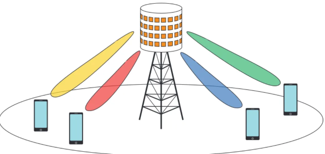
In this chapter, we introduce the basics of massive MU-MIMO uplink and downlink communications. A single-cell massive MU-MIMO system, as illustrated in Fig. 2.1, is considered. The system consists of a BS withBantennas that simultaneously servesU ≤

B single-antenna UEs in the same time-frequency resource using spatial multiplexing. Throughout this chapter, we shall assume, for simplicity, that the system operates over a frequency-flat channel and that all hardware components, including the ADCs and DACs, are ideal. The wireless channel connecting the UEs to the BS is modeled as memoryless block-fading channel, i.e., a channel that remains constant during a coherence interval of T = tcohfcoh consecutive symbol transmissions (channel uses), before changing into a new independent realization. Here, tcoh is the coherence time (measured in seconds) and fcoh is the coherence bandwidth (measured in Hertz). The average number of bits conveyed during a channel use is denoted byR and is called the rate(measured in bits per channel use or, equivalently, in bits per second per Hertz). A rate R is said to be achievable if there exist a sequence of codes operating at rate R for which the average error probability tends to zero as the length of the codewords tends to infinity. The channel capacity is defined as the supremum of all achievable rates [47, Chapter 3].

The rest of this chapter is organized as follows. In Sec. 2.1, we introduce the time-division duplexing (TDD) scheme used to separate uplink and downlink transmissions. In Sec. 2.2, we introduce the massive MU-MIMO uplink system model and provide the sum rate achievable with linear combing, Gaussian signaling, and perfect BS-side channel state information (CSI). In Sec. 2.3, we introduce the massive MU-MIMO downlink sys-tem model and provide the sum rate achievable with linear precoding, Gaussian signaling, and perfect BS-side CSI. Finally, we discuss channel estimation in Sec. 2.4.

Chapter 2 Fundamentals of Massive MU-MIMO

Figure 2.1:A single-cell multiuser MIMO system whereU single-antenna UEs are served by a

B-antenna BS in the same time-frequency resource through spatial multuplexing.

2.1 Time-Division Duplexing

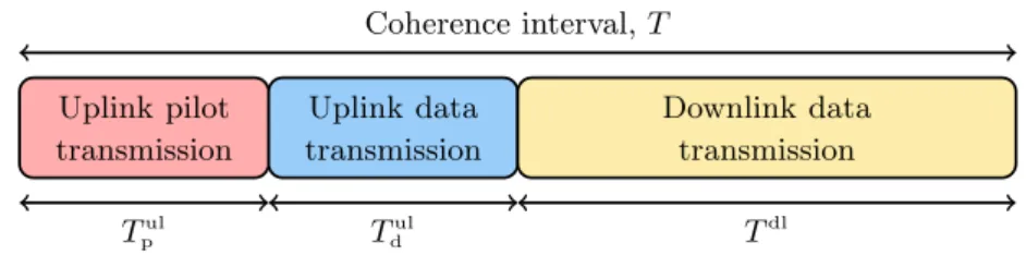
Throughout the thesis, it is assumed that the system operates in TDD mode, which implies that uplink and downlink transmissions take place in the same frequency spectrum but in different time slots. The TDD frame structure is illustrated in Fig. 2.2. We use

Tul _{and T}dl _{(for which it holds that T}ul_+Tdl _{=T) to denote the number of symbols} transmitted during the uplink and downlink phase, respectively. In every coherence interval, the UEs transmitTpul≥U pilot symbols (which are known to the BS) andTdul data symbols during the uplink phase (whereTul

p +Tdul=Tul). The pilot symbols allow the BS to acquire CSI, which, in turn, is used for detecting the data symbols. The CSI is also used for precoding theTdldata symbols transmitted from the BS to the UEs during the downlink phase.

2.2 Uplink Transmission

The discrete-time complex baseband signal received over theB BS antennas during the uplink phase of an arbitrary coherence interval can be written as

yul[n] =H sul[n] +wul[n] (2.1)

2.2 Uplink Transmission Uplink pilot transmission Uplink data transmission Downlink data transmission Coherence interval,T Tul p T ul d T dl

Figure 2.2:TDD frame structure. The UEs transmit pilots and data symbols in the uplink.

The BS transmits data symbols in the downlink.

for n = 0,1, . . . , Tul _{−1. Here, the vector s}ul_{[n] =}

sul

1[n], sul2[n], . . . , sulU[n] T

∈ CU,

which have independent and identically distributed entries, contains the symbols trans-mitted from all UEs. The transtrans-mitted symbols satisfies the average power constraint

E|sulu[n]|2

= Pul _{for u = 1,2, . . . , U, where P}ul _{is the UE transmit power. The} vec-tor wul_{[n] ∼ CN 0}

B×1, N0ulIB

is the BS-side additive white Gaussian noise (AWGN), where Nul

0 is the one-sided power spectral density (PSD) of the AWGN. Furthermore,

H ∈CB×U is the channel matrix. In what follows, we model the entries of H as

inde-pendent andCN(0,1)-distributed (Rayleigh fading).

In this section, we shall assume that the BS has noncausal access to perfect CSI, i.e., the BS knows perfectly the realizations of the channel matrix H. This assumption is reasonable only for very long coherence intervals, for which the pilot overhead can be ne-glected. For shorter coherence intervals, more pilot symbols will have to be transmitted to keep up-to-date with the time-varying channel. In this case, the rate loss associated with the transmission of pilots can not be neglected and perfect CSI can not be guaranteed.

With perfect CSI at the BS, the ergodic sum-rate capacity of the channel input-output model (2.1) is [48, Chapter 10] Cul=EH h log₂detIB+ SNRulHHH i (2.2) where SNRul=Pul_/Nul

0 is the uplink signal-to-noise ratio (SNR).

The sum-rate capacity in (2.2) can be achieved by performing minimum mean-square error (MMSE) together with successive interference cancellation (SIC) at the BS. Unfor-tunately, the computational complexity associated with implementing MMSE-SIC is pro-hibitively high, especially for massive MU-MIMO systems that simultaneously serve sev-eral UEs using a large number of BS antennas. Linear combining algorithms—although inferior to nonlinear processing algorithms such as MMSE-SIC—are less computationally demanding and, as will be shown next, yield near-optimal performance when the number of BS antennas exceed by far the number of UEs. With linear combining at the BS, an estimate zul[n] =

zul

1 [n], zul2[n], . . . , zulU[n] T

Chapter 2 Fundamentals of Massive MU-MIMO

obtained as follows:

zul[n] =Ayul[n]. (2.3)

Here,A∈CU×B is the combing matrix. It follows from (2.1) and (2.3) that

z_uul[n] =a_uThusulu[n] + X v6=u a_uThvsulv[n] +a T uw ul_{[n] (2.4)}

for u = 1,2, . . . , U. Here, hu ∈ CB is the uth column of H and au ∈ CB is the uth

column ofAT_{. The first term on the right-hand side (RHS) of (2.4) corresponds to the}

desired signal; the second term captures the MU interference; the third term corresponds to the AWGN.

It can be shown (see, e.g., [49, Eq. (12)]) that the sum rate achievable with Gaussian signaling and linear combing is

Rul= U X u=1 EH h log₂1 + SINRul_ui (2.5) where SINRul_u = SNR ul aT uhu 2 SNRulP v6=u|aTuhv| 2 +kauk22 (2.6)

is the uplink signal-to-interference-and-noise ratio (SINR) for theuth UE.

Three conventional linear combining schemes are maximal-ratio combing (MRC), zero-forcing (ZF) combing, and linear minimum mean-square error (LMMSE) combing [49]. The combing matrices associated with these schemes are

A=        HH_{, for MRC} HH_H−1 HH_{, for ZF} HH_H+ 1 SNRulIU −1 HH_{, for LMMSE.} (2.7)

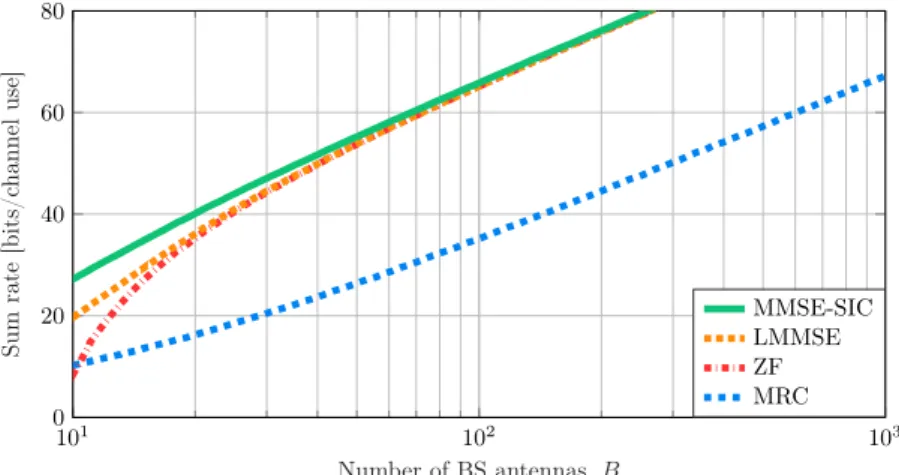
In Fig. 2.3, the sum rate achievable with Gaussian signaling and linear combing (2.5) is shown as a function of the number of BS antennas B for the case U = 10 UEs and SNRul = 0 dB. For reference, the rate achievable with MMSE-SIC (2.2) is also shown. Note that the rate achievable with ZF and LMMSE approaches the rate achievable with MMSE-SIC as the number of antennas grow large. This demonstrates that linear combing achieves near-optimal performance in the massive MU-MIMO uplink.

2.3 Downlink Transmission 101 ₁₀2 ₁₀3 0 20 40 60 80 Number of BS antennas,B Sum rate [bits/c hannel use] MMSE-SIC LMMSE ZF MRC

Figure 2.3:Uplink throughput for the case SNRul= 0 dB andU = 10 UEs. As the number of

BS antennas grow large, linear detection offers near-optimal performance.

2.3 Downlink Transmission

The discrete-time complex baseband signal received at the U UEs antennas during the downlink phase of an arbitrary coherence interval can be written as

ydl[n] =HTxdl[n] +wdl[n] (2.8) forn= 0,1, . . . , Tdl_{−1. Here,y}dl_{[n] =} ydl 1[n], ydl2[n], . . . , ydlU[n] T ∈_CU _{is the received}

signal at the U UEs and wdl[n] ∼ CN(0U×1, N0dlIU) is the AWGN at the UEs, where

Ndl

0 is the one-sided PSD of the AWGN. The transmitted signal over theBBS antennas,

xdl[n]∈CB, must satisfy the average power constraint EHkxdl[n]k22

≤Pdl. (2.9)

The capacity of the multiuser downlink channel has been characterized in [50–53]. When perfect CSI is available at the BS, dirty-paper coding (DPC) [54] is known to achieve the sum-rate capacity of the channel (2.8). The ergodic sum-rate capacity of the channel input-output model (2.8) is [55, Eq. (5)]

Cdl=EH " sup diag(t)0U×U,ktk22≤1 log2 detIB+ SNRdlHdiag(t)HH # (2.10)

where SNRdl=Pdl/N₀dl is the downlink SNR.

Practical implementations of DPC (see, e.g., [56–58]) are, however, computationally demanding, with a complexity that scales unfavorably with the number of BS antennas.

Chapter 2 Fundamentals of Massive MU-MIMO

Linear precoding on the other hand, is an attractive low-complexity approach to massive MU-MIMO precoding, which offers competitive performance to DPC for large antenna arrays [25]. With linear precoding, the transmitted signal can be written as

xdl[n] =αPsdl[n] (2.11)

whereP∈CB×U is the precoding matrix andsdl[n] =s1dl[n], sdl2[n], . . . , sdlU[n] T

∈CU,

wheresdl

u[n] is the symbol intended for theuth UE. These symbols are mutually

orthog-onal and adhere to the average power constraint_E |su[n]|2

=Pdl _{for u= 1,2, . . . , U.} Furthermore,α∈Ris chosen to satisfy the power constraint (2.9), i.e.,

α=_EHtr PPH −1/2

. (2.12)

It follows from (2.8) and (2.11) that

ydl_u[n] =αh_uTpusdlu[n] + X v6=u αhT_upvsdlv[n] +w dl u[n] (2.13)

for u = 1,2, . . . , U. Here, pu ∈ CB corresponds to the uth column of the precoding

matrixP. The first term on the RHS of (2.13) corresponds to the desired signal; the second term captures the MU interference; the third term corresponds to the AWGN. It can be shown (see, e.g., [59, Eq. (12)]) that the ergodic sum-rate achievable with Gaussian signaling and linear precoding is

Rdl=_EH " _U X u=1 log₂1 + SINRdl_u # (2.14) where SINRdlu = SNRdlhuTpu 2 SNRdlP v6=u|hTupv| 2 + 1/α2 (2.15)

is the downlink SINR for theuth UE. Here, we have assumed that the effective channel gainαhT

upu∈Cin (2.13) is known to theuth UE.

Three conventional linear precoders are maximal-ratio transmission (MRT), ZF pre-coding, and LMMSE precoding. The precoding matrices associated with these linear precoders are P=        H∗, for MRT H∗ HT_H∗−1 , for ZF H∗ HT_H∗₊ U SNRdlIU −1 , for LMMSE. (2.16)

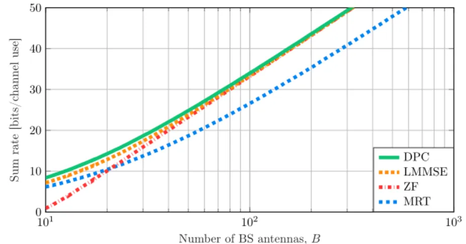
In Fig. 2.4, the sum-rate achievable with linear precoding (2.14) is shown as a function

2.4 Channel Estimation 101 ₁₀2 ₁₀3 0 10 20 30 40 50 Number of BS antennas,B Sum rate [bits/c hannel use] DPC LMMSE ZF MRT

Figure 2.4:Downlink throughput for the case SNRdl= 0 dB andU = 10 UEs. As the number

of BS antennas grow large, linear precoding offers near-optimal performance.

of the number of BS antennasB for the caseU = 10 and SNRdl= 0 dB. For reference, the rate achievable with DPC (2.10) is also shown (for the case of equal power allocation to the UEs). As the number of BS antennas grow large, the rate achievable with ZF and LMMSE precoding approaches the rate achievable with DPC, which demonstrates that linear precoding is near-optimal for large antenna arrays.

2.4 Channel Estimation

The uplink and downlink rates reported in (2.2), (2.5), (2.10), and (2.14) are valid for the case of perfect CSI at the BS. In practice, however, the channel realizations are not knowna priori to the BS. Therefore,Tpul≥U symbol transmissions are reserved for the transmission of pilot symbols, which are used at the BS to perform channel estimation. Let S=

sul_[0],sul_{[1], . . . ,s}ul_[Tul p −1]

∈ _CU×Tul

p _{denote the pilot symbols transmitted}

from the U UEs during the uplink training phase. The pilot sequences used by the different UEs are typically assumed to be mutually orthogonal, such that

SSH =TpulPulIU×U. (2.17)

With this assumption, the LMMSE estimate ofHis given by (see, e.g., [28, Sec. 3.1])

Hest= 1

Tul

p Pul+N0ul

Chapter 2 Fundamentals of Massive MU-MIMO where Y =HS+W and W = wul_[0],wul_{[1], . . . ,w}ul_[Tul p −1] ∈ _CB×Tul p _{. It follows}

that the channel matrixHcan be decomposed as (see, e.g., [60, Chapter 12])

H=Hest+E (2.19)

where the channel estimation errorE∈CB×U, which has independent and identically

dis-tributedCN(0, Nul

0 /(TpulPul+N0ul)) elements, is uncorrelated with the channel estimate

Hest_{. Note that channel estimation is performed separately at each antenna element.} Hence, the quality of the channel estimate improves with the number of pilot symbols and with the SNR, but not with the number of antenna elements.

The channel estimate Hest _{is used instead of H to compute the linear combining} matrix in (2.7) and the linear precoding matrix in (2.16), which will, inevitably, reduce the achievable rate since the channel estimates are not perfect. Furthermore, the pilot overhead will incur additional rate loss. Uplink and downlink rates achievable with imperfect CSI and linear processing have been reported in, e.g., [49, 59].

The results in this chapter are valid for massive MU-MIMO systems that are equipped with ideal hardware components. In practice, however, massive MU-MIMO systems will have to make use of nonideal hardware components, which will reduce the signal quality due to hardware impairments. For the remainder of the thesis, it will be assumed that the BS is equipped with low-resolution ADCs and DACs.

CHAPTER

3

Data Converters

Digital signal processing (DSP) is an integral part of all modern cellular systems. In the massive MU-MIMO uplink, in order to process data digitally, the analog signal re-ceived at each BS antenna is converted into the digital domain—a process that involves discretization in both time and amplitude. The device that performs these operations is called an ADC. Conversely, in the massive MU-MIMO downlink, the digital representa-tion of the transmit signal at each BS antenna is converted into an analog waveform by a DAC before being transmitted over the wireless channel.

3.1 Quantization

The process of converting a continuous-amplitude signal into a discrete-amplitude signal is known asquantization. We define aQ-bit quantizer by a set of 2Q _{quantization labels} L={`0, `1, . . . , `2Q₋₁}and a set of 2Q+ 1 quantization thresholdsT ={τ₀, τ₁, . . . , τ₂Q}, where−∞=τ0< τ1<· · ·< τ2Q=∞. Lety∈_Rdenote the input to the quantizer and letr∈ Ldenote the corresponding output. The output of the quantizer is

r=Q_R(y) (3.1) where Q_R(y) = 2Q₋₁ X q=0 `q1[τq,τq+1)(y) (3.2)

Chapter 3 Data Converters −2 0 2 −2 0 2 Input O ut pu t

(a)1-bit quantizer.

−2 0 2 −2 0 2 Input O ut pu t

(b)3-bit uniform quantizer.

−2 0 2 −2 0 2 Input O ut pu t

(c)3-bit nonuniform quantizer.

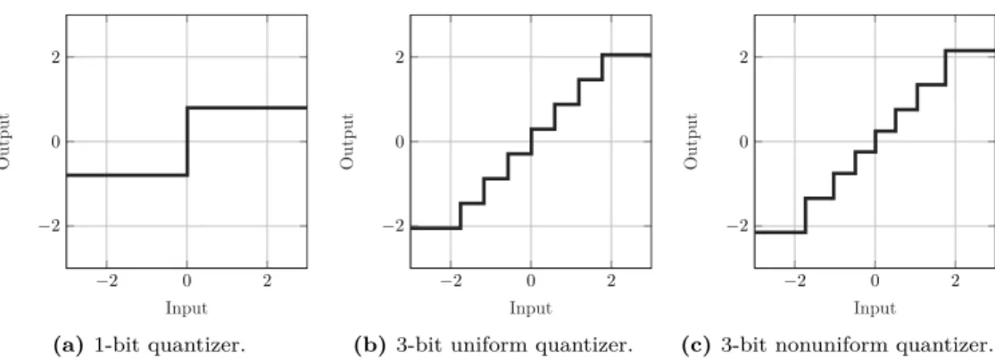
Figure 3.1:Input-output relation for (a) a 1-bit quantizer, (b) a 3-bit uniform quantizer, and

(c) a 3-bit nonuniform quantizer.

denotes the real-valued quantization function, which is applied element-wise to vectors. The quantizer is said to be symmetric and uniform if the quantization labels are

`q = ∆ q−2Q−1+ 1/2 forq = 0,1, . . . ,2Q−1 and if the quantization thresholds are

τq = ∆ q−2Q−1

for q = 1,2, . . . ,2Q _{−1. Here, ∆ is the step size of the uniform}

quantizer. If these conditions are not fulfilled, the quantizer is said to benonuniform. For uniform quantizers, the quantization function in (3.2) simplifies to

Q_R(y) =            ∆ 2 1−2 Q , ify <−γ ∆y ∆+ 1 2 , if 2Q _{is odd and|y|< γ} ∆_∆y+∆₂, if 2Q is even and |y|< γ ∆ 2 2 Q₋₁ , ify > γ. (3.3)

Here,γ = ∆2Q−1 is the clipping level of the uniform quantizer. If the number of quan-tization labels is odd, the uniform quantizer has a label at zero and is called amidtread quantizer. If the number of quantization levels is even, the uniform quantizer has a threshold at zero and is called amidrise quantizer. For the extreme case of 1-bit quan-tization, the quantization function in (3.3) reduces to

Q_R(y) =∆

2 sgn(y). (3.4)

Fig. 3.1 shows the input-output relation for a 1-bit quantizer (Fig. 3.1a), a 3-bit uniform quantizer (Fig. 3.1b), and a 3-bit nonuniform quantizer (Fig. 3.1c).

The process of mapping a continuous-amplitude signal into a finite set of quantization labels will inevitably introduce a quantization error

e=r−y. (3.5)

3.1 Quantization

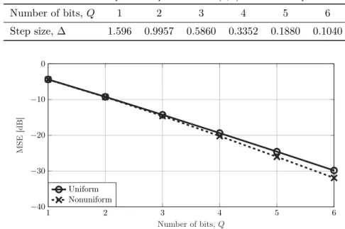
Table 3.1:MSE-optimal step size for aN(0,1)-distributed input.

Number of bits,Q 1 2 3 4 5 6 Step size, ∆ 1.596 0.9957 0.5860 0.3352 0.1880 0.1040 1 2 3 4 5 6 −40 −30 −20 −10 0 Number of bits,Q MSE [dB] Uniform Nonuniform

Figure 3.2:MSE after uniform and nonuniform quantization of aN(0,1)-distributed input.

The step size ∆ impacts the amount of error caused by a uniform quantizer. If ∆ is too small, then there will be significant overload distortion (i.e., the error|e|>∆/2 caused by inputs for which it holds that |y| > γ). On the other hand, if ∆ is too large, then there will be excessivegranular distortion (i.e., the error|e| ≤∆/2 caused by inputs for which it holds that|y| ≤γ). The mean square error (MSE) between the quantizer input and output is defined as MSE = _Ey

(r−y)2

. The MSE-optimal choice of step size depends on the PDF of the input to the quantizer [61]. In this work, we shall commonly consider quantization of Gaussian signals. For Gaussian-distributed inputs, the step size that minimizes the MSE is, in general, not available in closed form but can easily be found using numerical methods (see, e.g., [62, 63]). Table 3.1 lists the MSE-optimal step size fory∼ N(0,1) and for Q∈ {1,2, . . . ,6}.

At this point, it is important to note that uniform quantizers are, in general, subopti-mal. To demonstrate this, we show in Fig. 3.2 the MSE after uniform and nonuniform quantization of a N(0,1)-distributed input. For the case of uniform quantization, the step size is set according to Table 3.1. For the case of nonuniform quantization, the MSE-optimal set of quantization labels L and quantization thresholds T are obtained using the Lloyd-Max algorithm [63, 64]. It becomes clear that the performance gap between uniform quantization and nonuniform quantization grows larger as the number of bits increase. However, for low-resolution (e.g., 1–3 bits) quantizers, nonuniform quantization offers only marginal improvements compared to uniform quantization.

Chapter 3 Data Converters −1 0 1 0 0.2 0.4 0.6 0.8 1 Quantization error,e Probabilit y densit y Simulated U(−0.798,0.798)

(a)1-bit quantizer.

−1 0 1 0 0.3 0.6 0.9 1.2 1.5 Quantization error,e Probabilit y densit y Simulated U(−0.498,0.498)

(b)2-bit uniform quantizer.

−0.5 0 0.5 0 0.5 1 1.5 2 2.5 Quantization error,e Probabilit y densit y Simulated U(−0.293,0.293)

(c)3-bit uniform quantizer.

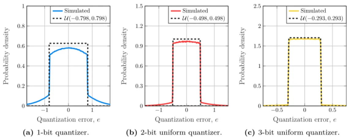
Figure 3.3:PDF of the quantization error for aN(0,1)-distributed input. Approximating the

quantization error as a uniformly distributed random variable becomes increasingly accurate as the number of bits grow large but is not an accurate approximation for low-resolution uniform quantizers.

A commonly adopted model for the error caused by a uniform quantizer is to approx-imate it as a noise term that is uncorrelated with the input and uniformly distributed in the interval [−∆/2,∆/2], such that the PDF ofeis (see, e.g., [65, Chapter 1.3], [66–69], and [70, Chapter 4.8]) fe(e)≈ (₁ ∆, − ∆ 2 < e < ∆ 2 0, otherwise. (3.6)

This approximation is sometimes called the pseudo-quantization noise (PQN) model [71]. Letσ2

y = Eyy2 and σe2 =Eee2 denote the variance of the input and the

quantiza-tion error, respectively. Note that MSE = σ2

e for zero-mean inputs. Furthermore, let

ρye=Ey[ye]/(σyσe) denote the correlation between the input and the quantization error.

According to the PQN model, it holds thatσ_e2 ≈ 1 ∆

R∆/2

−∆/2e

2_{de= ∆}2_{/12 and ρ}

ye ≈0.

Next, we shall discuss the validity of the PQN model for the case of uniform quantization of Gaussian signals.

In Fig. 3.3, we compare the PDF of the quantization error e with the approxima-tion (3.6) fory ∼ N(0,1) and for MSE-optimal uniform quantizers with Q ∈ {1,2,3} bits. We observe that the PQN model becomes increasingly accurate as the number of bits grow large. However, for low-resolution quantizers, there is a large discrepancy between the PDF according to the PQN model and the true PDF. In particular, we note that the quantization error is not contained within the interval [−∆/2,∆/2] for Gaussian signals. Indeed, for finite-resolution quantizers, there will always be overload distortion for input signals that have infinite support.

3.1 Quantization 0 0.5 1 1.5 2 2.5 3 0 0.2 0.4 0.6 0.8 1 Step size,∆ V ariance, σ 2 e PQN:σ2 e= ∆2/12 1-bit quantizer 2-bit uniform quantizer 3-bit uniform quantizer MSE-optimal step size

(a)Variance of the quantization error as a func-tion of the step size.

0 0.5 1 1.5 2 2.5 3 −1 −0.5 0 0.5 1 Step size,∆ Correlation, ρye PQN:ρye= 0 1-bit quantizer 2-bit uniform quantizer 3-bit uniform quantizer MSE-optimal step size

(b)Correlation between the input and the quan-tization error as a function of the step size.

Figure 3.4:Variance of the quantization error and correlation between the input and the

quan-tization error for a uniform quantizers and aN(0,1)-distributed input. The PQN model becomes increasingly accurate as the number of bits grow large but is not an accurate approximation for low-resolution uniform quantizers.

In Fig. 3.4, we show the variance σe2 and the correlation ρye as a function the step

size ∆ for y ∼ N(0,1) and for uniform quantizers with Q∈ {1,2,3} bits. Also shown are the approximations σ2

e ≈ ∆2/12 and ρye ≈ 0 according to the PQN model We

start by noting from Fig. 3.4a that, for 1-bit quantization, the PQN model significantly underestimates the variance of the quantization error. We further note from Fig. 3.4b that quantization error is, in general, correlated with the input signal. In particular, if the step size is set to minimize the MSE, there is a nonzero correlation between the input and the quantization error.

We conclude from Fig. 3.3 and Fig. 3.4 that the widely-adopted PQN model is not a suitable approximation for the quantization error caused by low-resolution (e.g., 1–3 bits) quantizers fed by Gaussian-distributed signals.

So far, we have only considered quantization of real-valued signals. For complex-valued signals y ∈C, it is commonly assumed that the real and imaginary components of the

input are quantized independently. In this case, the quantized signal can be written as

r=Q_C(y) (3.7)

where

Q_C(y) =Q_R(<{y}) +jQ_R(={y}) (3.8)

Chapter 3 Data Converters

Anti-aliasing

filter Sampling Quantizer

Analog input

Digital output

Figure 3.5:Block diagram of the basic functions of an ADC [65, Fig. 1.1a].

3.2 Analog-to-Digital Converters

A block diagram of the basic functions of an ADC is shown in Fig. 3.5. The process of converting a continuous-time signal into a discrete-time signal is known as sampling. Let fsamp denote the sampling rate of the ADC, which is measured in samples per second (SPS). To ensure that the input to the sampling circuit adheres (at least ap-proximately) to the sampling theorem, the analog input signal is passed through an anti-aliasing filter (a low-pass filter) prior to the sampling circuit. Throughout this the-sis, we shall assume that the anti-aliasing filter is an ideal low-pass filter with a cut-off frequencyfcutthat equals half the the sampling rate, i.e., fcut=fsamp/2 such that any out-of-band (OOB) interference present in the analog input does not enter into the sam-pling circuit. We shall also assume that the samsam-pling circuit is ideal (i.e., that there is no sampling-time jitter).

The discrete-time, continuous-amplitude output of the sampling circuit is fed toQ-bit quantizer, whereQis the resolution of the ADC (i.e., the number of ADC bits). While the sampling operation incurs no loss of information for band-limited signals. we recall from Sec. 3.1 that the nonlinear mapping of a continuous-amplitude signal into a finite set of possible labels introduces an error between the input and output of the quantizer, which can be made smaller by increasing the resolution of the ADC.

In an ideal ADC, the quantizer is the only source of distortion. Real-world ADCs, however, introduce additional noise and distortion caused by, for example, sampling-time jitter, integral nonlinearity, differential nonlinearity, and thermal noise [72, Chapter 6]. The effective number of bits (ENOB), which is defined as [65, Eq. (2.6)]

ENOB = SNDR [dB]−1.76

6.02 (3.9)

is a widely used performance measure for real-world ADCs. Here, SNDR is the signal-to-noise-and-distortion ratio (SNDR), which is defined as the root-mean-square of the input to the ADC divided by the power of the noise and distortion terms that are present in the output of the ADC. Some comments on (3.9) are in order. For the case when an ideal

Q-bit uniform quantizer is fed by a full-scale sinusoidal input γsin(2πf t+φ), where γ

is the clipping level of the quantizer, by using the PQN approximation (3.6), the SNDR