Production Networks

Production Networks

Kenan Huremovic, Fernando Vega-Redondo

To cite this version:

Kenan Huremovic, Fernando Vega-Redondo. Production Networks. 2016. <halshs-01370725>

HAL Id: halshs-01370725

https://halshs.archives-ouvertes.fr/halshs-01370725

HAL is a multi-disciplinary open access archive for the deposit and dissemination of sci-entific research documents, whether they are pub-lished or not. The documents may come from teaching and research institutions in France or abroad, or from public or private research centers.

L’archive ouverte pluridisciplinaire HAL, est destin´ee au d´epˆot et `a la diffusion de documents scientifiques de niveau recherche, publi´es ou non, ´emanant des ´etablissements d’enseignement et de recherche fran¸cais ou ´etrangers, des laboratoires publics ou priv´es.

Working Papers / Documents de travail

WP 2016 - Nr 33

Production Networks

Kenan Huremovic

Fernando Vega-Redondo

Production Networks

Kenan Huremovi´c

Aix-Marseille University (Aix-Marseille School of Economics), CNRS, & EHESS, Fernando Vega-Redondo

Bocconi University & IGIER First version: October 2014 This version: September 2016

Abstract

In this paper, we model the economy as aproduction network of competitive firms that interact in a general-equilibrium setup. First, we find that, at the unique Wal-rasian equilibrium, the profit of each active firm is proportional to (a suitable gener-alization of) its Bonacich centrality. We also determine consumer welfare at equilib-rium and characterize efficient networks. Then we proceed to conduct a broad range of comparative-static analyses. These include the effect on profits and welfare of: (a)distortions (e.g. tax/subsidies) imposed on the whole economy or specific firms; (b)structural changes such as the addition of links and the elimination of nodes; (c)productivity andpreference changes.

We discover that the induced effects are in general nonmonotone, depend on global network features, and impinge on each sector depending on the pattern of incentrali-tiesdisplayed by its input providers and output users. Furthermore, the inter-sector “linkages” underlying these effects can usually be decomposed – following the heuris-tic dichotomy proposed by Hirschman (1958) – into aforward (push) component and a backward (pull) one. Finally, we undertake some preliminary analysis of firm dy-namics and illustrate that, when evaluating policies of support and shock mitigation from a dynamic viewpoint, the reliance on strictmarket-based criteria can be quite misleading in terms of social welfare.

JEL:C67, D51, D85

1

Introduction

Any modern economy is a complex network of interfirm buyer-seller relationships that con-stitute its production structure. There is a growing interest among economists in adopting this network perspective to study a wide variety of economic phenomena: trade, interme-diation, innovation, technological diffusion, learning, or the transmission of shocks. This, of course, has prominent precursors in the celebrated work of John von Neumann, Wassily Leontief or Albert O. Hirschman, all of whom stressed the importance of interindustry relationships (or linkages) for a proper understanding of some of the key characteristics of an economic system. In this tradition, the present paper proposes a general-equilibrium model of the economy that, despite being standard in almost every respect, highlights the network of interfirm relationships on its production side. In a nutshell, our objective is to obtain a precise understanding of how the details of theproduction network topology (on which noa priori restrictions are imposed) shapes profits, welfare, and the effects (static and dynamic) induced by wide variety of changes and policy interventions.

In order to focus our analysis on the production structure of the economy, the demand side is modeled through a representative consumer while the technology of each firm is assumed of the Cobb-Douglas type. In general, however, each firm uses a diverse range of inputs, whose productivities are individually specific. Under these conditions, our analysis starts by showing that a unique equilibrium exists that displays a very sharp relationship to the network structure of the economy. Specifically, we find that, at equilibrium, the profitability of any given firm is proportional to its network centrality, as given by a suitable generalization of the well-known measure of centrality proposed by Bonacich (1987)1. On the other hand, we also determine the consumer’s welfare at equilibrium, providing closed expressions for how it depends on the different parameters of the model (in particular, the density and symmetry of the production structure).

Next, the paper turns to studying how the equilibrium is affected by a wide variety of different changes in the environment. First, we consider the impact of distortions, for-mulated in the idealized form of price wedges – either general ones that affect uniformly the whole economy, or individual ones applying to single firms. Then, we turn our at-tention to structural changes in the production network and consider both the effect of global transformations that affect either connectivity or the number of nodes, as well as local changes that affect only single nodes or individual links. We then close this part of our analysis with a comparative study of supply-channeled changes (such as technological improvements) with those that operate through variations in demand (e.g. a rise or fall

1_{For example, as compared to the received notion of Bonacich centrality that considers the paths of}

different lengths that join any given pair of nodes, in our case only those that connect a firm node to a consumption node are considered. The weight attributed to each of these paths reflects not only its length (as in the standard Bonacich centrality, they are discounted by their respective length) but also the relative importance that the consumer’s utility function attributes to the end good in question (while in the standard notion all end nodes are given a uniform weight).

in the consumer’s relative preference for a particular consumption good).

For all of the cases listed above, we provide formal expressions that capture the total impact of the change in an explicit form. These expressions are conceptually quite simple and should prove helpful in evaluating empirically alternative measures of economic policy. Furthermore, many of them can be understood in a quite parallel fashion, in that they involve a similar integration of constituent effects. Thus, on the one hand, they can be regarded as consisting of a first-order impact on the immediate agent experiencing the change (e.g. the firm subject to an individual tax or subsidy), followed by a spread of such a first-order impact throughout the whole network as captured by a suitable matrix of incentralities. On the other hand, the impact of many of those changes can also be decomposed in terms of a push effect that operates downstream and a pull effect that does so upstream. This dichotomy is reminiscent of the distinction between forward and backward linkages often considered in policy analysis and notably proposed by Hirschman (1958). Here we show how to distinguish precisely between them and also compare their implications: while forward linkages induce resource reallocation downstream but have no effect on profits, revenues, or input demands because of the entailed adjustment of prices, backward linkages alter significantly all those variables – i.e, not only prices but also revenues, profits, and input demands.

The analysis advanced so far is inherently static, i.e. it compares how different changes in the parameters of the model affectequilibrium magnitudes. By building on it, however, we can also address some genuinely dynamic issues. In this paper, we simply outline the problem, leaving for future work an exhaustive study of it. We consider, specifically, the problem of how to guide the distribution of firm support when, in the absence of it, some incumbent firms may go bankrupt and disappear. The key dynamic concern here is that, when several firms are at stake and not all can be supported, what particular firms are chosen may lead to subsequent effects that are drastically different. For, as one firm is protected but other fails, the latter may generate a cascade of ensuing failures that has major longer-run effects. The question then is: what is the best criterion to use if the objective is to minimize the overall (intertemporal) impact? In particular, we may ask: are current prices and induced profits the right market signal? In brief, the answer we provide is that, in some cases, profitability may by itself be a very misleading criterion and that other network-based criteria (embodying considerations of intercentrality) will, in general, be much more appropriate.

We end this short introduction with a brief review of related literature. From a methodological viewpoint, our approach is close to recent work by Acemoglu et al. (2012) who, building upon a Cobb-Douglas model proposed by Long and Plosser (1983), study how/whether microeconomic shocks on individual agents or sectors may aggregate into generating significant aggregate effects at the macroscopic level. Previous papers by Horvath (1998), Gabaix (2011) are motivated by a similar concern. As already explained,

our objective in this paper is very different and so are some of the key assumptions and questions asked. Thus, just to mention one significant difference, we do not make the assumption of constant returns in production since we are interested in how profit performance is affected by network structure. Besides, our analysis focuses on the effect of distortions, structural changes, or different kinds of demand and support policies rather than the spread of shocks, which are very different kind of phenomena.

Our work is also related to Jones (2011) who, building as well on the framework introduced by Long and Plosser (1983), studies how misallocation at the sector level affects GDP. More generally, our paper relates to the vast literature that has attempted to understand the intersectorial basis of economic development and the sectorial) policies that can mitigate either misallocation or/and coordination problems. The workhorse in this literature has been the input-output methodology originally formulated by Leontief (1936), which has spawned a huge body of work, both theoretical and empirical (see e.g. the monograph Miller and Blair (2009) for a recent account). Early on, building upon this rise of input-output analysis, the influential work of Hirschman (1958) highlighted the importance of some of the notions (e.g. forward and backward linkages) that will help us understand key forces underlying our model. In contrast with the traditional input-output literature, Hirschman’s approach emphasizes unbalanced growth rather than equilibrium as the primary tool ofdynamic analysis. To adopt such a perspective is also our eventual objective, even though in the present paper our analysis is still mostly static.

However, the preliminary dynamic analysis of evolutionary market forces undertaken in the last part of the paper (cf. the summary above) embodies some of the considerations implicitly highlighted by Hirschman’s work. It also hints at the role that network-based processes of propagation – e.g. of default through failure cascades – should have in a proper assessment of economic policy in a complex interconnected economy. This, in turn, leads us to the rich and diverse literature on contagion – for example, financial contagion – that has experienced a significant impetus in recent years (see the recent Handbook edited by Bramoulle et al. (2016) and the recent interesting work by Baqaee (2015) on the specific context of production networks). A different, and complementary, aspect in the dynamic study of economic networks concerns the processes of endogenous (payoff-guided) network formation. The network-formation literature is still in too-preliminary a state to provide much help in this endeavor. Our analysis of how certain structural changes on nodes and links affect agents’ payoffs is a very preliminary step in this direction. The recent paper by Oberfield (2012) studies a stylized version of the problem where agents endogenously select their production techniques, conceived as links that connect them to a unique supplier.

The rest of the paper is organized as follows. First, in Section 2 we present the bench-mark model, followed in Section 3 by the introduction of a collection of basic results. These results include, specifically, an account of how the topological features of the

pro-duction network shape the corresponding outcomes (i.e. profits of the firms and utility of the consumer). Then, in Section 4 we study how different kinds of distortions (uniform or firm-specific) affect the allocation of resources and relative firm performance. In Sec-tion 5 we investigate how does the global structure of production network determine the production and the welfare potential of the economy and howlocal perturbations in the network structure impinge on the equilibrium outcomes. Section 6 discusses the influ-entialpush-pull dichotomy stressed by Hirschman (1958) through the lens of our model. In Section 7 we provide a preliminary exploration of issues pertaining to firm dynamics and point out that market signals can be quite misleading from the point of the long run welfare. We summarize our contribution and conclude in Section 8.

In Appendix A we include the formal proofs of our main results. Then, in the (on-line) Appendix B, we present the general case with unrestricted heterogeneity, while in Appendix C (also available online) we revisit the comparative-statics analysis on firm distortions when the system is closed and thus the monetary flows involved must be balanced.

2

Benchmark model

We model an economy consisting of a finite set of firms N = {1,2, ..., n} and a single representative consumer. Our focus, therefore, is on the interfirm production relationships – i.e. the production network – through which the economy eventually delivers the net amounts of consumption goods enjoyed by the consumer. In principle, we allow that any specific good may be consumed, used as an intermediate input in the production of some other good, or display both roles simultaneously.

The goods that provide some utility to the consumer are labeled consumption goods, and are included in the set M ⊂ N, withm =|M| and c = (c1, c2, ..., cm) representing

a typical consumption bundle. For simplicity, leisure is not in the set M and thus yields no utility. Thus the consumer’s endowment of labor (which is normalized to unity) will be inelastically supplied by the consumer and hence only has an instrumental role as a source of income. The consumer’s preferences over consumption bundles are represented by a Cobb-Douglas utility functionU(·) of the form

U(c) = m Y i=1 cγi i (1)

where each γi represents the weight that the consumer’s preferences attributes to

con-sumption good i.

Concerning production, we assume that there is a one-to-one correspondence between firms and goods (thus, in particular, we rule out joint production).2 The production of

2

each good k takes place under decreasing returns to scale, and requires both labor and intermediate produced inputs. The set of intermediate inputs that firm k uses in its production is denoted byN_k+, with nk=|Nk+|. Letlk stand for the amount of labor used

in the production of goodk and let (zjk)_j∈N+

k be the associated amount of intermediate goods. Then the amountyk of good kproduced by the homonymous firm is determined

by the production function fk : Rnk ×R → R which is taken to display the following

Cobb-Douglas form: yk =fk (zjk)_j∈N_k+;lk =Aklβkk    Y j∈N_k+ zgjk jk    αk (2)

where the vector (gjk)_k∈N reflects the intensity (assumed positive)

3 _{with which firm k} uses/requires its different inputs, and αk > 0 and βk > 0 are the output elasticities of

labor and intermediate inputs.4

It is convenient to view the intensitiesgjk of input use as reflectingrelativemagnitudes,

so unless mentioned otherwise we shall normalize the corresponding vector to satisfy

P

j∈Ngjk = 1 – in other words, we assume that the matrix G is column-stochastic. On

the other hand, we assume that the production technologies exhibit decreasing returns, hence we posit that αk +βk < 1. It is worth noting that the model allows for full

heterogeneity across firms k ∈ N, not only in their pattern of input use (gjk)_k∈N but

also in their production elasticities αk and βk. The latter heterogeneity, however, does

not raise particularly interesting issues and, therefore, for the sake of formal simplicity, in the main text we shall focus throughout on the case where αk = α and βk = β for

some common valuesα and β. A detailed analysis for the fully heterogeneous case may be found in the online Appendix B.

It is common in economic models to posit that more advanced technologies employ a wider range of intermediate inputs, this being conceived as a reflection of higher “produc-tion complexity.” Here we choose to formalize this idea in the way suggested by Benassy (1998) (see also Acemoglu et al. (2007)), setting the pre-factor of the production function as

Ak=nα_k+ν (3)

with α+ν > 0. With this formulation, it is easy to see that a positive value of the

this perspective, what our model describes is the behavior of a typical firm in its corresponding sector, all firms belonging to a given sector producing perfectly substitute goods. This, of course, is a classical way of rationalizing, and providing foundations for, competitive behavior in equilibrium, as postulated below (see also Definition 2 in Appendix A).

3

Ifgjk= 0 for some inputjused in the production of a certain goodk, such an input is neither useful

nor required ink’s production. Therefore, it might as well be ignored altogether and the corresponding linkjkeliminated from the production network.

4_{This formulation implies that labor and all intermediate inputs in N}+

k are essential in production.

When the production technology ofN_k+=∅, we interpretQ

j∈N_k+z gjk

jk ≡1, thus no production is possible

parameter ν corresponds to the case where a wider input range enhances productivity, while a negative value reflects the opposite situation.5

The inputsj∈N_k+used in the production of goodkcan be viewed as the in-neighbors of nodekin the production directed network Γ ={N, L}, where the setN of its vertices is identified with the set of firms and there is a directed edge (i, j)∈L whenever j uses goodias an input, i.e. iffgji >0. This is a discrete (binary) network that only provides a

qualitative account of theproduction structure of the economy. A full-fledged description of this structure is provided by the matrix of production intensitiesG= (gij)_i,j∈N, which

in turn can be regarded as the adjacency matrix of the directed weighted network that describes completely the production structure. The matrixG, together with the elasticity parametersα andβ, and the utility functionU(·) of the representative consumer jointly provide a full description of the economy. To study its performance we shall focus on the standard notion of Walrasian (or Competitive) Equilibrium (WE), which consists of a collection of prices and quantities that satisfy the usual optimality and market clearing conditions. More precisely, a WE is an array [(p∗, w∗),(c∗,y∗,Z∗,l∗)] such that the following conditions hold:

1. The consumption plan c∗ = (c∗₁, c₂∗, ..., c∗_m) maximizes U(c) subject to the budget constraint given by the wage and profit income the consumer earns.

2. The production plans given by the outputs y = (y∗₁, y∗₂, ..., y_n∗), the demands for produced inputs Z∗ = (z∗_ij)i,j∈N, and the labor demands l∗ = (l∗1, l2∗, ..., l∗n) are all

technologically feasible and maximize, for each firmi∈N, its respective profit. 3. The labor market and the markets for produced goods clear (i.e. supply equals

demand).

A rigorous formalization of WE is provided by Definition 2 in Appendix A. Since the economy satisfies the usual properties contemplated by General Equilibrium Theory, existence of a WE readily follows.

3

Basic results

The form of the production function (2) has the implication that (providedα and β are both positive) labor and at least one intermediate input are essential in the production of any good. No firm, therefore, can be active (i.e. achieve a positive production) unless it

5

To understand this heuristically, suppose that firm k has a total amount of money M to spend amongnk intermediate inputs used in the production of goodk. Then, if each input enters production

symmetrically and also bears the same price, firmkshould splitM equally among thenkinputs. Fixing

the amount of labor used, this implies that production must be proportional tonα+ν

k M α 1 nk α =nν kMα.

Thus, ifν >0 there are benefits from increasing the range of inputs used in production, and the magnitude ofν quantifies precisely this effect.

relies on some other active firm. This imposes a natural requirement of “systemic balance” on an economic system if all its firms are to be active. And such a condition not only has static implications but, as we shall see in Section 7, it entails dynamic consequences as well. Similar considerations have been found to be important in the evolution of many other systems – biological, ecological, or chemical – where some suitable notion of systemic balance is also key to its static stability and dynamic evolution.6

However, an important feature of economic systems that has no clear counterpart in other contexts is that, in a market economy, the “source of value” is not just internal to the production network but, crucially, is also “externally” dependent on consumers’ preferences. Preferences provide the standard to measure welfare and also determine the market value that shapes firm performance. To discuss this issue, it is useful to extend the directed production network Γ = {N, L} with an additional node c that stands for our representative consumer. This nodec has an in-link (j, c) originating in every node

j∈M that produces a consumption good. Such an extended network is denoted by ˆΓ. As a preliminary step in our analysis, we want to understand when, given a particular (extended) production structure ˆΓ, a particular firmican be active at a WE. To this end, we rely on the notion of Strongly-Connected Component (SCC). Let the notation j k

indicate that there is a directed path originating in j and ending in k. Then, a subset of nodes Q⊂ N is said to be a SCC if, from every pair of nodes j, k ∈ Q,j k. The following result specifies necessary conditions for some particular node to be active at a WE.

Proposition 1

Consider any firm i∈N that is active at some WE. Then we have:

(a)∃Q⊂N that defines a SCC of the (extended) directed networkΓˆ s.t. ∀j∈Q, ji; (b)ic.

Proof. See Appendix A.

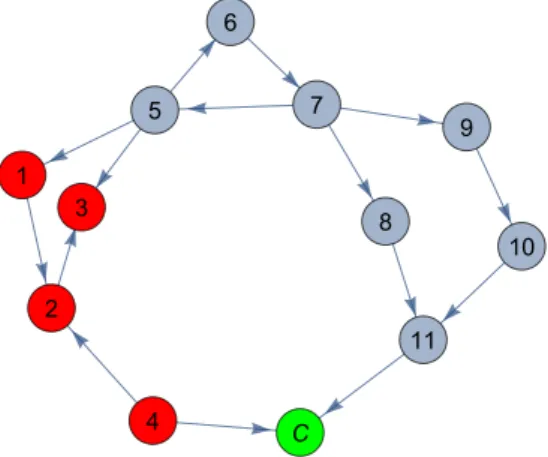
A simple illustration of the necessary conditions contemplated in Proposition 1 is provided by the production network shown in Figure 1. First we note that in this network the four firms/nodes coded in red – i.e. 1 to 4 – do not satisfy the necessary conditions (a)-(b) specified in Proposition 1 and thus cannot be active at any WE. The violation of these conditions occur because either they donot have any intermediate input to rely on (Firm 4) or there isnodirect or indirect connection to the consumer node (Firms 1 to 3). In the first case, the issue is one of feasibility (production of good 4 is not at all possible), while in the second case the problem is one of incentives (if the goods were produced, they would fetch no market value and hence lead to a zero profit).

In contrast, the remaining blue nodes 5-11 satisfy the aforementioned conditions and,

6

See, for example, the interesting work of Jain and Krishna (1998), who stress the importance of “autocatalytic balance” (the analogue of what we have called systemic balance above) in processes of growth in biological systems.

in principle, could be active at a WE. For nodes 5-7 this follows from the following two-fold observation: they define a SCC (so they jointly define a feasible production structure), and they also have an (indirect) connection to the consumer node (hence they may contribute to market value). Instead, firms 8 to 11 do not form part of a SCC, and thus have to depend on “external inputs” to undertake production. They can, however, obtain those inputs from the aforementioned SCC and then access market value through firm 11, which is connected to consumer nodec(i.e. produces a consumer good).

1 2 3 4 5 6 7 8 9 10 11 C

Figure 1: An extended production network ˆGthat includes the consumer node. The blue nodes are those that satisfy conditions (a)-(b) in Proposition 1, while the red ones do not. The green node represents the consumer demand.

Next, we address the question of whether there are conditions (possibly more stringent than those specified in Proposition 1) that are not only necessary but also sufficient, i.e. characterizewhen a firm is active at a WE. Building upon the ideas underlying Proposition 1 and the Cobb-Douglas specification of the model, we arrive at the following result.

Corollary 1

Consider any given firmi∈N. This firm is active at any WE if, and only if, it satisfies (a) and (b) in Proposition 1 and so happens as well for all other firms j∈N_i+ providing inputs to it.7

Proof. See Appendix A.

In view of the previous result, throughout this paper we shall assume that all existing firms satisfy (a)-(b). For short, this will be labeled Condition (A). Clearly, this condition can be assumed without loss of generality, for any other firm can be simply ignored in the analysis.

7_{Note that, clearly, if a goodisatisfies (b) in Proposition 1, then all its inputs satisfy it as well. Hence}

the only relevant requirement concerningi’s inputs is that they be supported from the production side, i.e. that they satisfy (a).

Of course, the identification of what firms are active at a WE provides only a very partial description of the situation. In general, there will be a wide heterogeneity in performance across firms (specifically, in terms of sales and profits). And if firms are symmetric in every respect except for their network position, it is the overall topology of the production network that should be used to explain such heterogeneity. Can we map the network-performance relationship in a sharp and insightful manner? To answer this question we turn to our first main result of the paper, Proposition 2 below.

Proposition 2

There exists a unique WE for which the vector of equilibrium revenues s∗ = (s∗_i)n_i=1 ≡ (p∗_i ·y_i∗)n_i=1 is given by

s∗ = w

∗_(1−α)

β (I−αG)

−1_{γ (i= 1,2, ..., n),}

while the corresponding equilibrium profits π∗ = (π_i∗)n_i=1 = (1−α−β)s∗.

Corollary 2

AssumeM =N (i.e. all goods are consumed). Then, the relativerevenues and profits of the different firms at the WE satisfy:

s∗_i Pn j=1s∗j !n i=1 = π ∗ i Pn j=1πj∗ !n i=1 = (1−α)(I −αG)−1γ.

Proofs. See Appendix A.

Proposition 2 establishes that – under the maintained condition (A) – the unique WE induces an equilibrium revenue (as well as profit) for each firmithat is proportional to a suitable measure of network centrality of this firm given by (I−αG)−1γ. As we explain next, this centrality notion integrates two main factors:

(i) the utility weight of each of the consumption goods whose production the firm’s output contributes to, either directly or/and indirectly;

(ii) a weighted discounted measure of the direct and indirect ways in which the afore-mentioned contribution takes place.

The measure of network centrality that arises from our analysis is a variation of the widely-used concept of Bonacich centrality. Since this notion of centrality is defined in the literature in slightly different forms, let us start our discussion by introducing the particular version to which we are referring here.

Definition 1

Consider a directed weighted network whose adjacency (n×n)-matrix is G. Let δ ∈(0,1) be a discount factor and ζ > 0 a scale factor. Then, the associated vector of Bonacich centralities is given by v(G, δ, ζ) = ζ(I −δG)−1_{1, where 1 is a suitable column vector}

To understand intuitively the notion of Bonacich centrality,8 suppose first that the network is binary, so that links either have a zero or unit weight, i.e. gij ∈ {0,1}for every

i, j ∈ N. Then, since the matrix G is assumed column-stochastic, its different columns have to include exactly one unit entry and the other entries must be equal to zero. In this simplified case, it is easy to show that the centrality of a particular node i can be interpreted as (is proportional to) the average of thediscounted number of pathsthat start at node iand reach all n nodes (including itself) in r steps (r = 1,2, ...). The discount factor used isδ ∈(0,1), and the total discount imposed on any given path is tailored to its length, i.e. it is δr if its length is r. To see this, rewrite the expression for centrality introduced in Definition 1 as follows:

v(G, δ, ζ) = (vi(G, δ, ζ))ni=1=ζ "_∞ X r=0 δrGr # 1 (4)

so that, for each i∈N, its corresponding centrality is given by

vi(G, δ, ζ) =ζ n X j=1 "_∞ X r=0 δrg[_ijr] #

where eachg_ij[r] represents theij-th entry of the matrixGr. The suggested interpretation is then a consequence of the fact that g[_ijr] simply counts the number of paths of exact length r that start at node i and end at node j. As we have seen (cf. Proposition 2), the discount factor to be used in our case is δ = α (where α is the output elasticity of intermediate inputs). Therefore, it turns out to be convenient to have a scale factor

ζ = (1−α)/n. Since the matrixG (and therefore every powerGr) is column-stochastic, this scaling amounts to normalizing the centrality vectorv to lie in then−1 simplex, i.e.

Pn

i=1vi= 1.

More generally, when the matrix G is a general column-stochastic matrix with its entries gij ∈ [0,1], an analogous interpretation can be provided but the “number of

paths” must then be replaced by the “normalized intensity” that flows between pairs of nodes for every possible path lengths. Applied to our production context, such intensity simply corresponds to the product of the input-demand flows between any given firm i

and the firmsj that use the former’s good as input, directly or indirectly.

The relationship between a firm’s performance and its Bonacich centrality is especially stark in the context considered in Corollary 2. There we abstract from any asymmetry associated to the consumption side: all produced goods are assumed to be consumption goods and equivalent for the consumer, which implies thatγ= 1_n1. Then, this result es-tablishes that therelativeperformance of firms isexclusivelydetermined by their Bonacich centrality in the production network for a discount factorδ=α and scale factor (1−α), where recall thatα is the production elasticity of intermediate inputs. In this sense, we

8

The measure introduced in Bonacich (1987) is defined by the expressionc(G, a, b) =b(I−αG)−1G1

may say that, given this elasticity, the profitability of a firm is the reflection of purely “topological” features of the production network.

In the general case where the vector of preferencesγis arbitrary and possiblyM 6=N

(not all goods are necessarily consumption goods), matters must be correspondingly adapted and the notion of centrality considered has to account for those asymmetries. Then, the relevant measure of centrality associates to the paths that arrive to any par-ticular nodej the weight γj that the consumer attributes to the respective good in her

utility function (cf. Proposition 2). Thus, in particular, if goodj is not a consumption good, paths of any given length r that connect some node i to such a node j do not contribute directly to the centrality (and therefore the profitability) of firmi. They may only do so indirectly to the extent that such paths can be constituent subpaths of longer ones that eventually connectito some consumption good k(in which case they would be weighted by γk and affected by a lower discount factor).

Having characterized the situation on the production side of the economy, now we turn to studying its consumption side. Specifically, our aim is to understand how the features of the network impinge on the consumer’s welfare at the WE. Again we find that the vector of centralities plays a prominent role, although in this case additional technological parameters are also important. We start the analysis by providing an explicit expression for theequilibrium utility in our next result.

Proposition 3

At the WE the consumer’s utility is given by logU(c) = n X i=1 γilogγi+ log(1−α)α α 1−α ₊ 1 1−α  (ν+α) X i vilogni−(1−α−β) X i∈N vilogvi+α X i∈N X j∈N_i+ vigjiloggji   (5)

where recall thatniis the number of inputs used in the production of goodi,ν is the

param-eter modulating the economies of scope through the factorAi=n_iα+ν, andv(G, α,1−α) =

(vi)ni=1 is the corresponding vector of Bonacich centralities for δ=α and ζ = 1−α.

Proof. See Appendix A.

The previous result highlights the threeendogenous magnitudes that shape welfare in our context:

1. The weighted average (log-)connectivity, P

ivilogni, where the degree of each

node/firm is weighted by its respective centrality.

2. A measure of heterogeneity/dispersion among firms, as reflected by the entropy of their centralities, (−P

i∈Nvilogvi).

3. The average heterogeneity/entropy in input use (i.e. −P

gjiloggji) displayed by

the technologies of the different firms i ∈ N, each of these individual magnitudes weighted by the centrality of the respective firmi.

4. The heterogeneity/entropy across goods,Pn

i=1γilogγi, displayed by the preferences of the representative consumer.

Specifically, we find that consumer welfare is increasing in the average log-connectivity of firms and ininter-firm symmetry, while it is decreasing in the intra-firm symmetry dis-played by their technologies. These different magnitudes are aggregated through a simple affine function whose coefficients are given by the underlying technological parameters.

Next, to obtain a sharper characterization of the situation, it is useful to reduce the degrees of freedom by postulating the following two symmetry assumptions:

(S1) For any given firmi∈N, its different inputs play a symmetric role in its production technology, i.e. gji =gki for all j, k ∈Ni+.

(S2) All goods are consumption goods and therefore γi = 1/n for every firmi∈N.

Under the previous conditions, the intra-firm heterogeneity of each firm i is dependent on ni alone, i.e. on the number of inputs it uses (which, heuristically, could be

under-stood as the “complexity” of its production technology). Then, the expression in (5) is substantially simplified, as stated by the following corollary.

Corollary 3

Assume (S1) and (S2) above. Then, the utility of the consumer at the WE is given by logU =−logn+ log (1−α)α1−αα ₊ 1

1−α ν n X i=1 vilogni−(1−α−β) n X i=1 vilogvi ! (6) Proof. See Appendix A.

Thus, under input symmetry, connectivity and inter-firm entropy are thesole considera-tionsthat impinge on consumer’s welfare. As we shall discuss in Subsection 5.1, this stark conclusion will allow us as well to obtain a similarly sharp assessment of what production structures are welfare optimal in different technological scenarios.

4

Price distortions

In this section, we focus on the study of what could be interpreted as taxes, distortions, or policy/price interventions of different sorts. An obvious, but still important, characteristic of an interconnected economy is that any such distortion or intervention cannot be studied just locally. In general, it is to be expected that its first-order impact could turn out to be quite different from its overall effect on the economy, once the complete chain of indirect effects is taken into account. Such a full-fledged analysis of the situation, however, can be very complex and we need effective tools to carry out a proper analysis of the situation. Here we provide a step in this direction.

Specifically, in this section we consider two different cases. First, in Subsection 4.1, we consider a price distortion that applies directly toall firms in the economy in a uniform manner. Then, in Subsection 4.2, we turn to studying distortions that apply directly to just one firm in the economy, so the effects on all others are only indirect. In both cases, uniform or individualized, we focus on situations that, at an abstract level, can be conceived as inducing “price wedges”. More concretely, this is an approach that can taken to capture a variety of different cases: government policies that favor a particular sector, ad-valorem taxes or subsidies, or the reflection of market power.9 To stress the intended generality, we shall simply speak of them asdistortions10.

A common idea that arises in the analysis of both uniform and individual distortion is that centrality-based measures are key in determining the size and direction of the induced effects. Centrality being an inherently global measure, the point is then that the impact of any change or intervention, no matter how “local” it might appear, must be evaluated globally. In fact, variants of the same general idea will reappear as well in much of the analysis conducted throughout the paper, again an indication of the unavoidable global nature of the issues being studied. In essence, the crucial network magnitudes involved in the analysis will turn out to be what we shall call (bilateral) in- and out-centralities. These are the elements of the matrix M = (mij)ni,j=1 ≡ (I −αG)−1 included in the definition of (Bonacich) centrality – cf. Definition 1.

Specifically, for every pair of nodes iand j, the ij-incentrality is identified with mij.

By writing vi(G, α, ζ) = 1−α n n X j=1 "_∞ X r=0 αrg_ij[r] # = 1−α n n X j=1 mij (7)

it is indeed apparent that mij represents (or, more precisely, is proportional to) the

contribution of nodej to the Bonacich centrality ofi. Reciprocally, we refer to the entry

mjias theij-outcentrality. Note that, within our general economic model (cf. Proposition

2), for each i∈N the entries mij (j= 1,2, ..., n) are the weights given to the preference

weightsγj of each good produced in the determination of the equilibrium profits of firm

ithrough the expression

π_i∗= (1−α−β)w ∗_(1−α) β n X j=1 mijγj. (8)

Thus, as explained, the contribution toi’s centrality provided by an intermediate product

j that is not consumed (whoseγj = 0) has no effect oni’s equilibrium profits.

9

See, for example, the paper by Hsieh and Klenow (2009) or Jones (2011) for an elaboration on such a general interpretation of price distortions.

10

Within our framework one can also analyze input specific distortions (i.e. distortions that lower the marginal product of one input relative to others, see (Hsieh and Klenow, 2009) for details) using the same tools. We do not include analysis of this type of distortions in the paper. The details are available upon request.

4.1 Uniform price distortion

We start our analysis of distortionary effects by considering the implications of a uniform price distortionτ imposed on all firms of the economy. Its effect is to draw a proportional wedge between the price pi the consumer pays for each good i and the price (1−τ)pi

received by the firm selling it. In principle, the value of τ might be negative, in which case it could be interpreted, for example, as a subsidy (hence amounting to a proportional increase in the revenue earned from the firm). An issue that arises here is whether the monetary payments (or proceeds) entailed should be distributed back to (or subtracted from) the revenue available to the agents of the economy – that is, whether the system is to be conceived as closed to those monetary flows. In general, the answer must depend on the specific interpretation attributed to those flows (e.g. on whether they are redistributive, or purely distortionary and hence wasteful). Here, in the main text, we shall consider the formally simpler case where they are a pure outflow (or inflow) of resources, while referring the reader to the online Appendix C for a consideration of the alternative closed-system version. None of our results are qualitatively affected by the scenario being considered.

Our first observation (see Lemma 1 in Appendix A for details) is that, under a uniform

τ applied to all goods of the economy, the expression that characterizes the vector of equilibrium profits is generalized to

π∗(τ) = (1−τ)(1−α−β)w(1−α)

β (I−α(1−τ)G) −1

γ (9)

This readily implies that, as expected, the effect on equilibrium profits of an increase in

τ is unambiguously negative – the reason, of course, is simply that, in our context, any distortion is always detrimental.11 Indeed, if we consider the marginal effect of increasing

τ, we find (see Lemma 2 in Appendix A): dπ∗

dτ (τ) =−(1−α−β)s

∗_{(τ)−α(I−α(1−τ)G)}−1_Gπ∗_(τ)<0

whereπ∗(τ) stands for the full vector of profits earned under τ by all firms.

Having settled the question of how a uniform distortion affects firms’ profits, next we turn our attention to the much more complex issue of how it candiversely impinges on the relative profits of the different firms, as a function of their individual position in the network. To account for this relative performance in a convenient manner, it is useful to focus on the normalized (equilibrium) profits (ˆπj)n_i=1 of each firm iobtained by

setting the nominal wage w(τ) so that P

j∈Nπˆj = 1. A formal characterization of the

(marginal) implications of changing τ on the relative profit performance of the different firms is provided by the following result.

Proposition 4

Given any given distortion τ ∈[0,1], let (ˆπj(τ))_i∈N be the corresponding profile of

nor-11_{An analogous conclusion obtains for the effect of τ on consumer’s welfare, which can be shown to be}

malizedequilibrium profits and denote ( ˜mij(τ))n_i,j=1 ≡(I−α(1−τ)G)−1. The marginal

effects on profits induced by a change on τ are determined by the following system of differential equations: dπˆi dτ (τ) = 1 1−τ n X j=1 ˜ mij(τ) (γj−πˆj(τ)) (i= 1,2, ..., n), (10)

and hence, at a situation with no distortion (τ = 0), the marginal impact of introducing it is: dπˆi dτ τ=0 = n X j=1 mij(γj−πˆj(0)) (i= 1,2, ..., n), (11)

where recall thatM = (mij)ni,j=1 is the matrix of incentralities.

Proof. See Appendix A.

The above result highlights that the firms most negatively affected in their relative profit performance by the introduction of the distortion are those whose centrality is heavily dependent on firms with high original profits. A particularly stark manifestation of this idea is displayed in (11), which applies to the case where the distortion is just being marginally introduced. This expression can be heuristically understood as follows. The effect on the relative profit standing of any given firm changes as prescribed by an average composition/multiplication of two magnitudes:

(a) the first-order impacts experienced by each one of the firms in the economy, whose sign and size is captured for each firmj ∈N by (γj−ˆπj(0)) – a comparison of firm

j’s relative profit and the (relative) weight of its output in consumer’s preferences; (b) the extent to which those impacts are transmitted to the firm i in question, as

captured by its respective vector ofij-incentralities (mij)nj=1.

When the base distortion is not zero but is some givenτ >0, this two-fold mechanism exhibits the general form given by (10), which has an analogous interpretation. An in-teresting feature of this expression is that the sensitivity of relative equilibrium profits to interfirm asymmetries grows steeply asτ approaches unity. Another interesting consider-ation worth highlighting is that, because the dependence of profits onτ is nonlinear, there is the potential for complex (and, in particular, nonmonotonic) behavior as the distortion changes within its full range [0,1]. The following simple example illustrates that this is indeed a possibility.

Example 1

Consider the simple production network with nine firms depicted in Figure 2, where it is assumed that all firms produce a consumption good and hence the arrows only indicate the flow of input use. Figure 3 traces the relative profits for possible values of τ ∈ [0,1]

and a subset of firms (for the sake of readability, not all firms are included). The second diagram shows that, asτ grows (and, naturally, the profit spectrum across firms narrows) there are rank changes in the relative position of some firms. Thus, while Firm 6 remains the highest-profit firm throughout, as τ grows the position of Firm 8 deteriorates, from second to fourth position. Indeed, we find that it is not just the ranking partially changes but even the relative profit of an individual firm may evolve in nonmonotonic way as τ

rises. Specifically, as shown more clearly in Figure 4, this happens to Firm 1, whose profit first grows and then decreases.

1 2 3 4 5 6 7 8 9

Figure 2: A simple production network illustrating the discussion included in Example 1.

0.0 0.2 0.4 0.6 0.8 1.0 τ 0.06 0.08 0.10 0.12 0.14 0.16 0.18 ˆ π

Firm 1

Firm 5

Firm 6

Firm 7

Firm 8

Figure 3: The relative profits of all firms in the production network displayed in Figure 2 for all values ofτ ∈[0,1].

0.0 0.2 0.4 0.6 0.8 1.0 τ 0.111 0.112 0.113 0.114 0.115 0.116 0.117 0.118 0.119 0.120 ˆ π

Firm 1

Figure 4: The nonmonotonic behavior of the relative profit of firm 1 in the production network displayed in Figure 2, asτ changes in the range [0,1].

4.2 Individual price distortion

In this subsection, our focus turns from a common distortion that affects uniformly all firms to one that impinges only on a specific firm k. As shown in Appendix A, such a firm-specific price distortion, denoted by τk, introduces just a simple modification in

the equilibrium expressions derived for the benchmark model, but one that is of a quite different nature from those obtained for a uniform distortion. For example, in contrast with (9), the induced equilibrium profitsπ∗(τ_ko) = [π_i∗(τk)]n_i=1 are now given by:

π∗(τk) = (1−α−β) w∗(1−α) β I−αGˆ(τk) −1 γ. (12)

where ˆG represents a modified matrix that replaces the original one, G. These matrices only differ in their respectivekth columns, ˆg_k and g_k, which satisfy ˆg_k= (1−τk)gk.

The difficulty lies in studying the inverse in (12) to obtain its dependence on τk. To

do this, it is useful to write the modified matrix ˆG(τk) as follows:

ˆ

G(τk) =G−τkgke0k, (13)

wheree0_k is then-dimensional row vector that has a 1 in itskth position and 0 elsewhere. This then allows us to rely on the following result in Linear Algebra (cf. Sherman and Morrison (1949) or Hager (1989)):

Sherman-Morrison Formula. LetAbe a nonsingularn-dimensional real matrix, and

c, dtwo real n-dimensional column vectors such that 1 +d0A−1_{c6= 0. Then,}

(A+cd0)−1 =A−1−A

−1_cd0 A−1

Applying the above result to our case – with the particularizationA=I−αG,c=τkgk,

andd=ek– we arrive at the following full characterization of how thek-specific distortion

affects equilibrium profits.

Proposition 5

Consider a distortionτk imposed on firm k and let (πi∗(τk))n_i=1 stand for the

correspond-ing equilibrium profits. The marginal effects on profits induced by a change on τk are

determined by the following system of differential equations: dπ∗_i dτk (τk) =−π∗k(0) mik (1−τk(1−mkk))2 (14)

and hence, at a situation with no distortion (τk = 0), the marginal impact of introducing

it is: dπ_i∗ dτk τk=0 =−π_k∗(0)mik (i= 1,2, ..., n), (15)

Proof. See Appendix A.

The previous result states that the profit decrease experienced by any firm i due to the direct distortion impinging on another firmkdepends on

• how profitablek was prior to the distortion;

• the importance ofk in determining the centrality ofi; • how much ofk’s centrality “feeds into” itself.

As intuition would suggest, while the first two considerations increases the profit loss on firmidue to distortion onk, the last one decreases it (with the only exception considered in (15) when there is no distortion to start with). Again we observe that incentralities (as captured by themik and mkk mentioned in the last two items) play a prominent role

in shaping the overall global effect. It is also interesting to observe from (14) that the function mappingk’s distortion into i’s profit is convex so that, just as in the uniform-distortion case, the marginal effect of increasing τk grows with the level of it. Another

feature that was noted for the previous uniform case is that the induced nonlinearities can lead to somewhat paradoxical conclusions. This phenomenon arises as well here, as illustrated below by through two examples.

Example 2

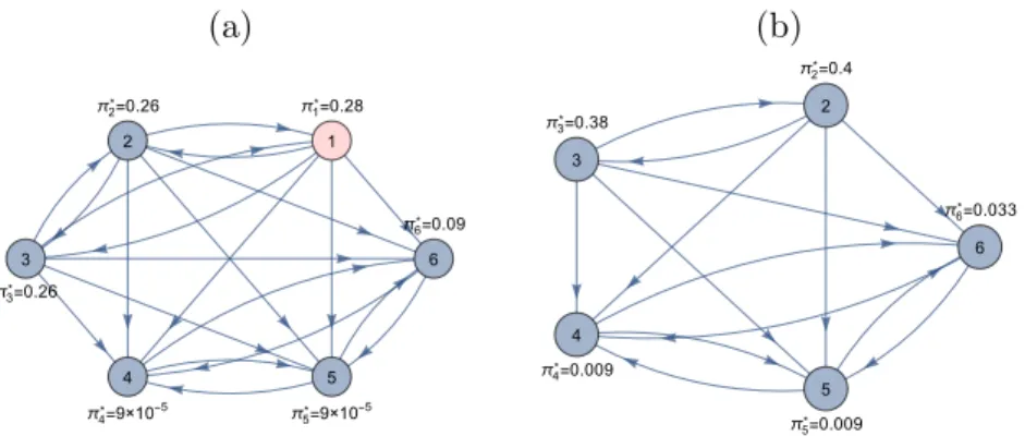
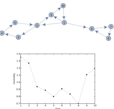
Consider the production network depicted in Figure 5, where the corresponding profile of Bonacich centralities are also shown. Again, for simplicity, all produced goods are assumed to be not only intermediate inputs but consumption goods as well. Firm 1 and then Firm 2 are those with the highest centrality in the production network. Therefore, under no distortion, they are also the firms enjoying the highest profits at the Walrasian equilibrium.

1 2 3 4 5 6 7 8 9 10 1 2 3 4 5 6 7 8 9 10 Firm 0.7 0.8 0.9 1.0 1.1 1.2 1.3 1.4 Centrality

Figure 5: A production network in the upper panel, with the corresponding profile of Bonacich centralities for each of the nodes displayed in the lower panel.

However, as shown in Figure 6, the situation can change in interesting ways if our focus turns to relative profits (normalized to add up to one) and the distortion τ2

expe-rienced by Firm 2 varies. (Note that here we are allowing τ2 to be negative, varying in

the range τ2 ∈ [−1,1] and thus playing possibly the role of a subsidy.) For τ2 = 0 (no

distortion) the profit ranking exactly mimics that of centralities, as already explained. In contrast, asτ2 grows and becomes positive, we observe the somewhat paradoxical fact that

the relative profit of Firm 2 monotonically grows and, eventually, if τ2 is high enough,

even surpasses that of Firm 1 and becomes the highest. The opposite state of affairs is found if Firm 2 is subject to a negative τ2. Then, a higher absolute value for it induces

a lower profit for this firm, eventually leading it to fall below that of Firm 10. Why does this happen? The reason is that, as the distortion varies, the effect of this change – which is modulated by the various incentralities – impinges most strongly on the those firms i

whose i2-incentrality is highest, which then alters the relative position of Firm 2 in the direction opposite to the change ofτ2. A further illustration of this role of incentralities,

1.0 0.5 0.0 0.5 1.0 τ2 0.04 0.06 0.08 0.10 0.12 0.14 0.16 0.18 ˆ πi

Firm 1

Firm 2

Firm 3

Firm 5

Firm 10

Figure 6: The change in relative profits among the firms placed in the production network depicted in Figure 5 as the distortion experienced by Firm 2 changes in the range [−1,1].

Example 3

Suppose that ten firms are arranged into a ring production network with each firm i = 1,2, ...,10 using the good produced by Firmi−1 as the sole intermediate input and having its produced good be the sole intermediate input in the production of Firmi+ 1(of course, indices0 and 11 are interpreted as 10 and 1, respectively). As in the previous examples, all produced goods are assumed to be valuable to the consumer. Consider now a distortion experienced by Firm1, τ1 ∈[−1,1]. 1.0 0.5 0.0 0.5 1.0 τ1 0.02 0.04 0.06 0.08 0.10 0.12 0.14 ˆ πi

Firm 1

Firm 4

Firm 6

Firm 8

Firm 10

Figure 7: The change in relative profits among the firms placed in a ring production network of ten firms as the distortion experienced by Firm 1 changes in the range [−1,1]. In such a ring network, the input links define the cycle 1→2→3→...→10→1.

vari-ation of τ1. The most affected is Firm 10, either negatively if τ1 > 0 or positively if

τ1<0. The reason is that this firm is the one with the highest i1-incentrality. Following

it, the firm whose bilateral incentrality relative to1 is the highest is Firm9, and thus this firm is the one which is the second most affected by changes in τ1, and so on along the

ring. In the end, we find that, indeed, the firm that is least affected is Firm 1, the firm that is directly subject to the distortion. Of course, this stark conclusion is an artifact of the extreme production network considered but should help clarify the key mechanism underlying global effects in our context.

5

Network structure

In line with our core concern of understanding how economic structure affects perfor-mance, here we undertake an analysis of the following issues. First, in Subsection 5.1, we study what features of the production structure (e.g. whether it is more or less con-nected, or its degree of heterogeneity) impinge on the production and welfare possibilities attainable at equilibrium. Then, in Subsections 5.2 and 5.3, our focus turns to study-ing the overall effect of sstudy-ingle “local perturbations” affectstudy-ing the production structure. Specifically, we consider two of them: (i) the creation (or elimination) of a linkij; (ii) the elimination of an existing node/firm, or the creation of a new one. As we shall explain, these changes can be understood as reflecting alternative economic phenomena.

5.1 Optimal network structure

The structure of production networks can be studied along many different dimensions. Here we show that, as far as its impact on (consumer) welfare is concerned, theinternode symmetry displayed by the network and its connectivity stand out as two key features. To highlight their effect, it is useful to simplify the analysis by focusing on networks that satisfy the assumptions (S1)-(S2) introduced at the end of Section 3. That is, we postulate that (a) the inputs involved in the production of every good play a symmetric role, and (b) all goods are consumption goods. We also suppose that the number of goods in the economy is given, while postponing to Section 7 an analysis of what are the welfare implications of a change in this feature of the economy. Under these conditions, we can build upon the analysis undertaken in Section 3 to arrive readily at the following conclusion.

Proposition 6

Assume (S.1)-(S.2) in Section 3. Then, the production structure that maximizes consumer utility is a regular network (i.e. all firms have the same number of inputs). Furthermore, if ν > 0 the optimal network is complete (i.e. for all i ∈ N, ni = |N_i+| = n−1),

i∈N, ni = 1).

Proof. See Appendix A.

The previous result follows from inspection of the expression determining equilibrium utility in (6), as a function of the the parameters of the economy and the induced profile of firm centralities. On the one hand, the last term of that expression calls for the maximization of the entropy of the simplex-normalized vector of centrality profiles, as given by−P

i∈Nvilogvi. This maximization is attained when all nodes have the same

centrality, which in turn requires that the network be symmetric across nodes and hence regular. Thus all firms must display the same “input complexity,” i.e. they should all use the samenumber of inputs. Then, whether such common complexity should be maximal or minimal sharply depends on the sign of the parameterνin (3), which reflects the nature of the “economies of input scope” in production. If ν > 0, complexity is beneficial and hence the optimal production structure should be complete, i.e. all other goods should be used in the production of every one of them. Instead, ifν <0, the exact opposite applies and the optimal production structure should display the minimum complexity consistent with viability (cf. Corollary 2). That is, it should constitute a ring for example.

In principle, of course, it is far-fetched to entertain the possibility that the production structure of the economy might be “designed.” Instead, it is more natural to conceive this structure to be a reflection of a wide number of different forces (e.g. technological change or any other modification of the underlying economic environment) whose magnitude and direction can hardly be controlled. Therefore, the discussion in this subsection has to be interpreted mostly as a conceptual exercise. That is, the objective is to gain some under-standing of what features of the production structure of an economy have an important impact on welfare. And, from this perspective, what Proposition 6 shows is that (abstract-ing from some other considerations) two characteristics arise as key: symmetry across all production processes and extreme exploitation/avoidance of all economies/diseconomies of scope.

5.2 Link creation

In the remaining part of this section, we adopt a local perspective to the analysis of changes in the production structure. First, in this subsection, we focus on the impact of a change affecting a single link – for concreteness, we consider the case where the link is created. A preliminary and immediate point to note is that if a linkij is formed, the firm

i that consequently sees an expansion in the uses of its output cannot have its relative profits decrease. The reason is that its centrality cannot decrease by this change – clearly, the set of paths that access consumer nodes can only grow.

inputs has increased – is in general ambiguous (see Example 4 below). It depends, for example, on how the weights (gkj)_k∈N_j+ are affected by the change. Among the different

possibilities one could contemplate in this respect, here we shall assume, for concreteness, that the new matrix ˜Gcontinues to be column stochastic. A possible interpretation of this modeling choice is that the new link entails a new and full-fledged production technology available to firmjthat, if adopted by this firm, satisfies the same normalization condition as all other technologies do. In a sense, we view it as embodying a mature new option that can be selected by firmj as a coherent and balanced package.12

Proposition 7

Consider an initial production network with adjacency matrix G and suppose that a link

ij is added to it. Denote by G˜ the resulting adjacency matrix and let q= (qk)nk=1 ∈ Rn

(P

k∈Nqk = 0) be the real vector that reflects the entailed adjustment across the two

adjacency matrices, i.e. their respectivejth columns,(gkj)n_k=1 and (˜gkj)n_k=1, satisfy˜gkj =

gkj +qk for all k = 1,2, ..., n with ˜gij = qi > 0. The change on equilibrium profits,

(∆π_k∗)n_k=1, induced by the new link is given by: ∆π_k∗ =α π_j∗ mkiqi+P_{`∈N</sub>+ j mk`q` 1 +qimji+αP<sub>`∈N}+ j mj`q` , (16)

where π_j∗ is the original profit of firm j under adjacency matrix G. Proof. See Appendix A.

The previous result establishes that if a new linkij is added to the production network, the effect on the equilibrium profit of any particular firmj is given by the composition of two key factors:

• The profit originally obtained by the firmj that provides a new use to goodi. Intu-itively, this magnitude reflects the importance of firmj in providing the immediate market value generated by the new linkij.

• The impact on the centrality ofkof each of the inputs involved in the production of

j (including the new inputi), as captured by the respective incentralities,mki and

(mk`)<sub>`</sub>∈N_j+. Each of these incentralities is weighted by the factor q` that reflects the

adjustment made (positive or negative) when transforming the adjacency matrixG

into ˜G.

Again, therefore, we can understand the changes resulting from the new link as consisting of the composition of two kinds of effects: afirst-order effect whose magnitude is

associ-12

Admittedly, this is only one of the possibilities that could be reasonably considered. Alternatively, it could be assumed that the components of the new (˜gkj)_k∈N+

j

sum up to some positive magnitudeH6= 1. Then, one could still unit-normalize the correspondingj-th column of ˜Gby adjusting the overall input elasticity of firmj to the value ˜αj =Hαj. None of these possible modeling variations would affect the

ated to the equilibrium-induced importance of the directly affected nodes; asecond-order effect that involves the transmission of the aforementioned first-order effect through the full array of network-based interactions that are captured by the matrix of incentralities.

Example 4

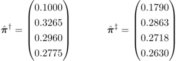
As advanced, in this example we illustrate that the addition of a new linkij can deteriorate the relative position of the firm whose input range is expanded by the new link. Consider the production networks depicted in Figure 8, and suppose that the smaller network gives rise to the larger one that includes the new link 1→4. Let us assume that all goods are consumer goods and have an equal weight in the utility function of the consumer. Let us also suppose that the new matrixG˜ displayed after the change continues being column stochastic. Then, denoting by ˆπ† and πˆ‡ the respective vectors of normalized profits for the original and modified networks, we compute them to be as follows:

ˆ π†=       0.1000 0.3265 0.2960 0.2775       ˆ π‡=       0.1790 0.2863 0.2718 0.2630       (17)

Thus one finds that firm 4 obtains a lower relative profit after the link 14 is added to the original network. Why is this the case? The simple reason is that, as explained, centrality (and hence profitability) is associated to the (discounted) value a product delivers to the consumer, not to the value it allows other firms to attain. That is, profitability is gathered downstream rather that upstream and, given architecture of the network in our example, the discounted downstream “flow” gained by Firm 4 from the new link falls relative to that of the other firms – in particular, that of Firm 1, whose centrality is sure to increase.

1 2 3 4 1 2 3 4

Figure 8: Two different production networks, whose only difference concerns the existence, or not, of the link from node 1 to node 4. All nodes/firms are supposed to produce a consumption good with equal preference weights.

5.3 Node deletion

In this section, we study the alternative (local) change in the production structure given by the addition or removal of a (single) node rather than those of a link. Now, for concreteness, we focus our attention on the case where the change involves the removal

of the node. This is, in fact, the kind of change that will be considered in Section 7 when studying the chain implications of a process of node/firm bankruptcy and endogenous removal.

Once more we must face the modeling question of how the setup is to be renormalized when the network changes – in this case, the set of nodes. Now it concerns both the utility and the production functions, all of which deliver a value of zero when any of its arguments is equal to zero. For the utility function, the renormalization we choose to tackle the problem is the natural one: we restrict its arguments to the range of consumer goods which can actually be produced given the prevailing set of active firms. In Subsection 7.1, we provide a specific motivation for this choice in a context where the number of firms changes due to a process firm selection.

Concerning the renormalization to be implemented on the production functions when there is a reduction in the inputs available, again for concreteness we choose one specific option but other alternatives could be analogously considered. The alternative considered is different from that adopted in Subsection 5.2, where the change involved an increase in input use. As we now explain, this contrast is motivated by a different view on what is the nature of the phenomenon underlying the situation in either case. Here we conceive the disappearance of a node as a somewhat abrupt/unexpected event that requires some short-run and hence partial adjustment. Thus, unlike what was suggested for the case of link creation, we assume that the columns of the matrixGare not renormalized. Thus the firmsjthat see one of its inputs vanish somehow adapts (for otherwise the indispensability of all prior inputs would force it to a zero production) but in a partial manner. Along with the point made in Footnote 12, we can interpret this as a downward shift in the productivity in the overall use of the available intermediate inputs.13 Admittedly, one should not expect real-world situations to be so markedly polar as suggested between the increase and decrease in the use of preexisting inputs. The contrast, however, is plausible and we find it useful to simplify the discussion of either case.

Before stating the main result from this subsection, let us introduce following notation. Let ˜G denote the resulting adjacency matrix after deletion of nodei. If the deleted firm produced a consumption good, then after deletion of that node one may expect that weightsγ that the consumer’s preferences attribute to all remaining goods will adjust14. Let ˜γ denote the vector of resulting preference weights after a node is deleted.

In view of the relationship established between profitability and centrality, it is quite clear that the elimination of a node can only be detrimental to the profits of all firms in the economy. A precise specification of the relative magnitudes of the effects that apply to each of them is given by the following result.

13_{If we proceeded in this way, a full-fledged analysis of the situation should rely on the extended}

framework considered in the online Appendix B, where full firm heterogeneity is allowed – in particular, on input elasticities.

14

Proposition 8

Consider an initial production network with adjacency matrix G and suppose that node

i∈N ={1,2, ..., n} is removed from it. Denote by ∆π∗_j

j6=i the change in equilibrium

profits of the remaining firms. Then,

∆π∗_j(G) = ˜πj(G)−π∗j(G)−π˜i(G)

mji(G)

mii(G)

, (18)

where π˜(G) = (1−α−β)1−_βαw∗(I−αG)−1γ˜ Proof. See Appendix A.

The previous result indicates that the effect induced by the removal of a particular firmion the profits of the remaining firmsj6=iexhibits the usual pattern: a first-order effect (that is quantified by the prominence/profitability of the firm directly affected, i.e. firmi) composed with the effect that the directly affected firm has on the centrality of any other firm (measured by the corresponding incentrality). In the present case, however, the incentrality terms mji are “normalized” by the effectmii that firm i has on its own

centrality – in this sense, the relevant magnitude scales the outcentralities of i by the extent to which this firm’s centrality effect feeds into itself. The additional effect, which may have an opposite sign, is due to potential preference adjustments and is captured by difference ˜πj(G)−πj∗(G). Note that when there is no adjustment in consumer’s preferences

(when ˜γj =γj ∀j∈ {1,2, .., n} \ {i}) equation (18) becomes

∆π_j∗(G) =−π_i∗(G)mji(G)

mii(G)

.

6

Forward and backward linkages

As explained in the Introduction, one of the useful features of the model is that it al-lows a transparent formalization of the notions of forward and backward linkages (also called push and pull effects) that, as stressed by (Hirschman, 1958), can be important in assessing, for example, public interventions and economic policies. In essence, all of the comparative static results considered so far in Subsections 4.1 through 5.3 can be conceived as involving those two types of linkages, forward and backward. That is, the overall effects considered so far can be seen to include a forward linkage that operates downstream on the production structure, and a backwards one that works upstream.

Rather that revisiting all our previous results in this light, it will prove more useful at this point to discuss these forces/linkages in the context of two particularly clear-cut instances: a (Hicks-neutral) pattern of technological improvements on the production technologies of the different firms; an arbitrary change in the preferences of the consumer across the different goods. As we shall see, while the first case exerts only pure “push” forces on the equilibrium outcome, the second one embodies an array of “pull” forces

(some positive and others negative).

6.1 Technological change

Consider a change in the pre-factors (Ak)k∈N of the production functions of each firmkin

the economy (cf. (2)-(3)), which become ( ˜Ak)k∈N. We shall refer to them as the

produc-tivities of the respective firms. The key observation to make from Proposition 2 is that the equilibrium conditions imply that the induced sales at equilibrium areindependent of those productivities. This readily leads to the following two conclusions:

(i) The equilibrium input demands [(z_jk∗ )j6=k]k∈N by each firmk(which are proportional

to sales) remain unaltered by the change in productivities. Thus, in this sense, there areno pull effects operating upstream along the production structure.

(ii) The equilibrium prices of the goods enjoying higher productivities decrease propor-tionally no less than their respective productivities rise. This in turn triggers a downstream push over all sectors that use those goods directly or indirectly, with lower prices all along inducing more output being produced.

Item (i) is quite clear and requires no further elaboration. It is worth mentioning, how-ever, that for the same reason why input demands are unaffected by the change, profits are unaffected as well. Productivity changes, therefore, have no effect on the inter-firm distribution of profits. The reason why this happens is highlighted in Item (ii). In the new equilibrium, price changes adapt to absorb all quantity effects (direct and indirect) resulting from increased productivities. This, to be sure, is crucially dependent on our Cobb-Douglas formulation, which implies that price changes exactly absorb all quantity effects (direct and indirect) resulting from increased productivities. Admittedly, such a consequence of the postulated functional form is quite extreme, but has the advantage of highlighting the contrast between forward and backward linkages in a clear-cut manner. A precise account of how these price-mediated effects propagate upstream is provided by the following result.

Proposition 9

Consider a set of changes in firm productivities such that the new levels, ( ˜Ai)i∈N, are

related to the former ones as follows: ˜

Ai =ξiAi (ξi >0, i= 1,2, ..., n). (19)

Under a suitable normalization, the corresponding equilibrium prices(˜p∗_i)i∈N and(pi)∗i∈N,

respectively prevailing before and after the change, satisfy: