Symmetry 2018, 10, 486; doi:10.3390/sym10100486 www.mdpi.com/journal/symmetry
Article
TODIM Method for Multiple Attribute Group
Decision Making under 2-Tuple Linguistic
Neutrosophic Environment
Jie Wang, Guiwu Wei * and Mao Lu
School of Business, Sichuan Normal University, Chengdu 610101, China; [email protected] (J.W.); [email protected] (M.L.)
*Correspondence: [email protected]
Received: 24 September 2018; Accepted: 8 October 2018; Published: 11 October 2018
Abstract: In this article, we extend the original TODIM (Portuguese acronym for Interactive Multi-Criteria Decision Making) method to the 2-tuple linguistic neutrosophic fuzzy environment to propose the 2TLNNs TODIM method. In the extended method, we use 2-tuple linguistic neutrosophic numbers (2TLNNs) to present the criteria values in multiple attribute group decision making (MAGDM) problems. Firstly, we briefly introduce the definition, operational laws, some aggregation operators and the distance calculating method of 2TLNNs. Then, the calculation steps of the original TODIM model are presented in simplified form. Thereafter, we extend the original TODIM model to the 2TLNNs environment to build the 2TLNNs TODIM model, our proposed method, which is more reasonable and scientific in considering the subjectivity of DM’s behaviors and the dominance of each alternative over others. Finally, a numerical example for the safety assessment of a construction project is proposed to illustrate the new method, and some comparisons are also conducted to further illustrate the advantages of the new method.
Keywords: multiple attribute group decision making (MAGDM); 2-tuple linguistic neutrosophic sets (2TLNSs); TODIM model; 2TLNNs TODIM method; construction project
1. Introduction
The Interactive Multi-Criteria Decision Making (TODIM) model, first defined by Gomes and Lima [1], is a useful tool to investigate multiple attribute group decision making (MAGDM) problems and has been widely used in industrial, commercial economy, and management science areas. Some traditional MAGDM models have been investigated in the previous literature, such as: the ELimination Et Choix Traduisant la Realité (ELECTRE) model [2]; the Preference Ranking Organization Method for Enrichment of Evaluations (PROMETHEE) model [3]; the Technique for Order of Preference by Similarity to Ideal Solution (TOPSIS) model [4,5]; the grey relational analysis (GRA) model [6–8]; the multi-objective optimization by ratio analysis plus the full multiplicative form (MULTIMOORA) model [9,10]; and, the VIseKriterijumska Optimizacija I KOmpromisno Resenje (VIKOR) model [11–13]. Compared with these existing methods, the TODIM model, which is based on prospect theory (PT), [14] has the advantages of considering the subjectivity of decision maker’s (DM’s) behaviors and providing the dominance of each alternative over others with particular operation formulas, and can be more reasonable and scientific in the application of MAGDM problems.
In practical decision problems, it is difficult to present the criteria values with real values for the complexity and fuzziness of the alternatives, and so it can be more useful and effective to express the criteria values with fuzzy numbers. Fuzzy set theory, which was initially introduced by Zadeh, [15]
has been proved as a feasible means in the application of MAGDM [16,17]. Smarandache [18,19] provided the neutrosophic set (NS). Then, Wang et al. [20,21] investigated theories about
single-valued neutrosophic sets (SVNSs) and provided the definition of interval neutrosophic sets (INSs). Ye [22] studied multiple attribute decision making (MADM) problems under the hesitant linguistic neutrosophic (HLN) environment. Wang et al. [23] studied the dual generalized Bonferroni mean (DGBM) aggregation operators under the SVNNs environment. Liu and You [24] proposed some linguistic neutrosophic Hamy mean (LNHM) aggregation operators. Wu et al. [25] gave the definition of SVN 2-tuple linguistic sets (SVN2TLSs) and proposed some new Hamacher aggregation operators. Ju et al. [26] extended the SVN2TLSs to the interval-valued environment and presented some single-valued neutrosophic interval 2-tuple linguistic Maclaurin symmetric mean (SVN-ITLMSM) operators. Wu et al. [27] studied SVNNs with Hamy operators under the 2-tuple linguistic variable environment. Wang et al. [28] provided the definition of the 2-tuple linguistic neutrosophic number (2TLNN) in which the degree of truth-membership, indeterminacy-membership and falsity-membership are depicted by 2TLNNs. Thereafter, the SVNS theory has been widely used to study MAGDM problems.
Gomes and Lima [1] used the TODIM model to investigate MADM problems taking the DM’s confidence level into account to obtain more rational selection under risk. Wei et al. [29] extended the TODIM method to the hesitant fuzzy environment. Ren et al. [30] studied the TODIM model under the Pythagorean fuzzy environment. Fan et al. [31] established an extended TODIM model to solve MADM problems. Wang and Liu [32] developed an extended TODIM model based on intuitionistic linguistic information. Krohling et al. [33] extended the original TODIM method to the intuitionistic fuzzy numbers environment to propose the IF-TODIM method, and Lourenzutti and Krohling [34] built an intuitionistic fuzzy TODIM model based on the random environment. Wang et al. [35] combined the TODIM method with multi-hesitant fuzzy linguistic information to propose a likelihood-based TODIM method. Liu and Teng [36] provided an extension of the TODIM method under the 2-dimension uncertain linguistic variable. Sang and Liu [37] extended the TODIM method to interval type-2 fuzzy environments. Pramanik et al. [38] provide the NC-TODIM method under the neutrosophic cubic sets. Xu et al. [39] considered both the traditional TODIM model and SVNSs to build the SVN TODIM and IN TODIM models. Hu et al. [40] proposed a three-way decision TODIM model. Huang & Wei [41] proposed the TODIM method for Pythagorean 2-tuple linguistic multiple attribute decision making. However, there has been no study about the TIDOM model for MAGDM problems with 2TLNNs and there is a need to take the 2TLNNs TIDOM model into account. The goal of our article is to combine the original TIDOM model with 2TLNNs to study MAGDM problems. The structure of our paper is as follows. Section 2 introduces the concepts, operation formulas, distance calculating method, some aggregation operators of 2TLNNs and the calculation steps of the original TODIM model. Section 3 extends the original TIDOM model to the 2TLNNs environment and introduces the calculation steps of the 2TLNNs TIDOM method. Section 4 provides a numerical example and introduces the comparison between our proposed methods and the existing method. Section 5 provides some conclusions from our article.
2. Preliminaries
2.1. 2-Tuple Linguistic Neutrosophic Sets
Based on the concepts of 2-tuple linguistic fuzzy set (2TLS) and the fundamental theories of the single valued neutrosophic set (SVNS), the 2-tuple linguistic neutrosophic sets (2TLNSs) first defined by Wang et al. [28] can be depicted as follows.
Definition 1 ([28]). Let 1, ,2 ,k be a linguistic term set. Any label
i shows a possible linguistic variable,and =
0=extremely poor,1=very poor,2=poor,3=medium, 4=good,5=very good,6=extremely good.
,(
)
(
) (
)
s
,
,
s
,
,
s
,
=
(1)where s s, ,s
, , , − 0,5, 0.5)
,(
s
,
)
,
(
s
,
)
and s
(
,
)
represent the degree of the truth membership, the indeterminacy membership and the falsity membership which are expressed by 2TLNNs and satisfies the condition
−1(
s
,
)
,
−1(
s
,
)
and
−1(
s
,
)
0,
k
,
(
)
(
)
(
)
1 1 1
0
−s
,
+
−s
,
+
−s
,
3
k
.Definition 2 ([28]). Assume there are three 2TLNNs
(
) (
) (
)
1 1 1 1
s
,
1,
s
,
1,
s
,
1
=
,(
) (
) (
)
2 2 2
2s
,
2,
s
,
2,
s
,
2
=
and
=
(
s
,
)
,
(
s
,
) (
,
s
,
)
, the operation laws of them can be defined:(
)
(
)
(
)
(
)
(
)
(
)
(
)
(
)
1 2 1 2 1 2 1 2 1 1 1 1 1 2 1 2 1 2 1 1 1 1 1 2 1 2 , , , , , ; , , , , , s s s s k k k k k s s s s k k k k k k
− − − − − − − − + − = (
)
(
)
(
)
(
)
(
)
(
)
(
)
(
)
(
)
(
)
1 2 1 2 1 2 1 2 1 2 1 1 1 2 1 1 1 1 1 2 1 2 1 2 1 1 1 1 1 2 1 2,
,
,
,
,
,
,
, ;
,
,
,
,
s
s
k
k
k
s
s
s
s
k
k
k
k
k
s
s
s
s
k
k
k
k
k
− − − − − − − − − −
=
+
−
+
−
(
)
1(
)
1( )
1,
,
,
1
1
s
,
s
,
s
,
0;
k
k
k
k
k
k
− − −
=
− −
(
)
1( )
1( )
1,
,
,
,
1
1
s
,
1
1
s
,
0.
s
k
k
k
k
k
k
− − −
=
− −
− −
According to Definition 2, it is clear that the operation laws have the following properties:
( )
( )
2( )
1 1 2 1 2 2 1,
1 2 2 1,
1 1
=
=
=
;
(2)(
1 2)
1 2,
(
1 2) ( ) ( )
1 2;
=
=
(3)(
) ( )
1( )
2( )
(1 2) 1 1 2 1 1 2 1,
1 1 1.
+
=
+
=
(4)Definition 3 ([28]). Let
=
(
s
,
)
,
(
s
,
) (
,
s
,
)
be a 2TLNN, the score and accuracy functions of
can be expressed:( )
(
2
1(
,
)
1(
,
)
1(
,
)
)
,
( )
0,1
3
k
s
s
s
s
s
k
− − −+
−
−
=
(5)( )
1(
)
1(
)
( )
,
,
,
,
h
=
−s
−
−s
h
−
k k
(6)For two 2TLNNs
1 and
2, based on Definition 3, then( ) ( )
( )
( )
( ) ( ) ( )
( )
( ) ( ) ( )
( )
( ) ( ) ( )
( )
1 2 1 2 1 2 1 2 1 2 1 2 1 2 1 2 1 2 1 2 1 2 1 2 1 2(1)
,
;
(2)
,
;
(3)
,
,
;
(4)
,
,
;
(5)
,
,
.
if s
s
then
if s
s
then
if s
s
h
h
then
if s
s
h
h
then
if s
s
h
h
then
=
=
=
=
=
2.2. The Normalized Hamming Distance
Definition 4. Let
(
) (
) (
)
1 1 1 1s
,
1,
s
,
1,
s
,
1
=
and
(
) (
) (
)
2 2 2 2s
,
2,
s
,
2,
s
,
2
=
be two 2TLNNs, then we can get the normalized Hamming distance:(
)
(
)
(
)
(
)
(
)
(
)
(
)
1 2 1 2 1 2 1 1 1 1 1 2 1 2 1 2 1 1 1 2,
,
,
,
1
,
3
,
,
s
s
s
s
d
k
s
s
− − − − − −
−
+
−
=
+
−
(7)Theorem 1. Assume there are three 2TLNNs
(
) (
) (
)
1 1 1 1
s
,
1,
s
,
1,
s
,
1
=
,(
) (
) (
)
2 2 2
2s
,
2,
s
,
2,
s
,
2
=
and
(
) (
) (
)
3 3 3 3s
,
3,
s
,
3,
s
,
3
=
, the Hamming distanced
has the following properties:( )
(
)
( )
(
)
( ) (
1 21)
2(
2 1)
( ) (
1 12) (
2 2 3)
1(
12 3)
P1 0
,
1;
P2
,
0,
;
P3
,
,
;
P4
,
,
,
.
d
if d
then
d
d
d
d
d
=
=
=
+
Proof.( )
P1 0
d
(
1,
2)
1
Since(
) (
)
1 2 1 1 1 2,
,
,
0,
s
s
k
− −
, then(
)
(
)
1 2 1 1 1 20
−s
,
−
−s
,
k
,
similarly we can get
(
)
(
)
(
)
(
)
1 2 1 2 1 1 1 1 1 2 1 2
0
−s
,
−
−s
,
k
, 0
−s
,
−
−s
,
k
, then(
)
(
)
(
)
(
)
(
)
(
)
1 2 1 2 1 2 1 1 1 1 1 1 1 2 1 2 1 20
−s
,
−
−s
,
+
−s
,
−
−s
,
+
−s
,
−
−s
,
3
k
, So(
(
)
(
)
(
)
(
)
(
)
(
)
)
1 2 1 2 1 2 1 1 1 1 1 1 1 2 1 2 1 20
−s
,
−
−s
,
+
−s
,
−
−s
,
+
−s
,
−
−s
,
3 .
k
( )
P2
if d
(
1,
2)
=
0,
then
1=
2(
)
(
( ) (
)
(
) (
)
( ) (
)
)
( ) (
)
(
) (
)
( ) (
)
(
)
( )
(
) (
)
(
) ( )
(
)
(
)
1 2 1 2 1 2 1 2 1 2 1 2 1 2 1 2 1 2 1 1 1 1 1 1 1 2 1 2 1 2 1 2 1 1 1 1 1 1 1 2 1 2 1 2 1 1 1 1 1 1 1 2 1 2 1 21
,
,
,
,
,
,
,
0
3
,
,
0,
,
,
0,
,
,
0
,
,
,
,
,
,
,
,
d
s
s
s
s
s
s
k
s
s
s
s
s
s
s
s
s
s
s
s
− − − − − − − − − − − − − − − − − −=
−
+
−
+
−
=
−
=
−
=
−
=
=
=
=
That means
1=
2, so( )
P2
if d
(
1,
2)
=
0,
then
1=
2 is right.( ) (
P3
d
1,
2)
=
d
(
2,
1)
(
)
(
( ) (
)
(
) (
)
(
) (
)
)
(
) ( )
(
) (
)
(
) (
)
(
)
(
)
1 2 1 2 1 2 2 1 2 1 2 1 1 1 1 1 1 1 1 2 1 2 1 2 1 2 1 1 1 1 1 1 2 1 2 1 2 1 2 1 1 , , , , , , , 3 1 , , , , , , , 3 d s s s s s s k s s s s s s d k
− − − − − − − − − − − − = − + − + − = − + − + − =So we complete the proof.
( ) (
P3
d
1,
2)
=
d
(
2,
1)
holds.( ) (
P4
d
1,
2)
+
d
(
2,
3)
d
(
1,
3)
(
)
(
)
(
)
(
)
(
)
(
)
(
)
(
)
(
)
(
)
(
)
(
)
(
)
(
)
(
)
(
)
(
)
(
)
1 3 1 3 1 3 1 2 2 3 1 2 2 3 1 2 2 3 1 1 1 1 1 3 1 3 1 2 1 1 1 3 1 1 1 1 1 2 2 3 1 1 1 1 1 2 2 3 1 1 1 1 1 2 2,
,
,
,
1
,
3
,
,
,
,
,
,
1
,
,
,
,
3
,
,
,
,
s
s
s
s
d
k
s
s
s
s
s
s
s
s
s
s
k
s
s
s
s
− − − − − − − − − − − − − − − − − −
−
+
−
=
+
−
−
+
−
=
+
−
+
−
+
−
+
−
(
)
(
)
(
)
(
)
(
)
(
)
(
)
(
)
(
)
(
)
(
)
(
)
(
)
(
)
(
)
1 2 2 3 1 2 2 3 1 2 2 3 3 1 1 1 1 1 2 2 3 1 1 1 1 1 2 2 3 1 1 1 1 1 2 2 3 1 2 2 3,
,
,
,
1
,
,
,
,
3
,
,
,
,
,
,
s
s
s
s
s
s
s
s
k
s
s
s
s
d
d
− − − − − − − − − − − −
−
+
−
+
−
+
−
+
−
+
−
=
+
□2.3. The Aggregation Operators of 2TLNNs
Definition 5 ([28]). Let
(
,
) (
,
,
) (
,
,
)
(
1, 2,
,
)
j j j
j
s
js
js
jj
n
=
=
be a group of 2TLNNs, then the 2TLNNWA and 2TLNNWG operators proposed by Wang et al. [25] are defined as follows.(
1 2)
1 1 2 2 12TLNNWA
,
,
,
=
n n n n j j j
=
=
(8) and(
) ( )
1( )
2( )
( )
1 2 1 2 12TLNNWG
,
,
,
=
n j n n n j j
=
=
(9)where
j is weighting vector of
j,
j
=
1, 2,
, .
n
which satisfies 10
j1,
n j1.
j
=
=
Theorem 2 ([28]). Let
(
,
) (
,
,
) (
,
,
)
(
1, 2,
,
)
j j j js
js
js
jj
n
=
=
be a group of 2TLNNs, then the operation results by 2TLNNWA and 2TLNNWG operators are also a 2TLNN where(
)
(
)
(
)
(
)
1 2 1 1 1 1 1 1 12TLNNWA
,
,
,
,
,
1
1
,
,
,
.
j j j j j j n n j j j w w n j n j j j w n j js
s
k
k
k
k
s
k
k
= − − = = − ==
−
−
=
(10) and(
)
( )
(
)
(
)
(
)
1 2 1 1 1 1 1 1 12TLNNWG
,
,
,
,
,
,
1
1
,
,
1
1
.
j j j j j j j n n j j w w n n j j j j w n j js
s
k
k
k
k
s
k
k
= − − = = − ==
−
−
=
−
−
(11)2.4. The Original TODIM Method
The TODIM method, which is based on prospect theory (PT), considers the subjectivity of DM’s behaviors and can provide the dominance of each alternative over others with particular operation formulas, and is more reasonable and scientific in the application of MAGDM problems.
Assume that
1,
2,
m
be a group of alternatives,
c c
1,
2,
c
n
be a list of criteria withweighting vector be
w w
1,
2,
w
n
, thereby satisfyingw
i
0,1
and1
1
n i i=
w
=
. Construct a decision matrix
=
d
ij m n whered
ij means the estimate results of the alternative(
1, 2,
,
)
i
i
m
=
based on the criterionc
j(
j
=
1, 2,
,
n
)
. Suppose thatw
jk=
w w
j k berelative weight of
c to c
j t wherew
k=
max
( )
w
jk j
,
=
1, 2,
,
n
. The traditional TODIMmethod decision making steps can be summarized as follows:
Step 1. Normalize ij m n
d
=
into ij m nd
=
.Step 2. Calculate the dominance degree of
i over each alternative
t based onc
j. Let
be the attenuation factor of the losses. Then
(
i,
t)
nj 1 j(
i,
t)(
i t
,
1, 2,
,
m
)
(
)
(
)
(
)
(
)
1 10
,
0
0
1
0
n jk ij tj j jk ij tj j i t ij tj n jk ij tj jk ij tj jw
d
d
w
if d
d
if d
d
w
d
d
w
if d
d
= =
−
−
=
−
=
−
−
−
(13)where
j(
i,
t)
(
d
ij−
d
tj
0
)
means gain and
j(
i,
t)
(
d
ij−
d
tj
0
)
indicates loss.Step 3. Compute the overall value of
( )
i with formula (14):( )
(
)
(
)
(
)
(
)
1 1 1 1,
min
,
max
,
min
,
m m i t i t i t t i m m i t i t i i t t
= = = =
−
=
−
(14)Step 4. To choose the best alternative by rank the values of
( )
i , the alternative with maximum value is the best choice.3. The TODIM Method with 2TLNNs
Assume that
1,
2,
m
be a group of alternatives,
d d
1,
2,
d
be a list of expertswith weighting vector be
v v
1,
2,
v
t
, and
c c
1,
2,
c
n
be a list of criteria with weighting vectorbe
w w1, 2, wn
, thereby satisfyingw
i
0,1 ,
v
i
0,1
and 11,
11
n t i i i=
w
=
i=v
=
. Construct a decision matrixr
ij m n
=
where
(
,
) (
,
,
) (
,
,
)
ij ij ij ijs
ijs
ijs
ij
=
means theestimate results of the alternative
i(
i
=
1, 2,
,
m
)
based on the criterionc
j(
j
=
1, 2,
,
n
)
by expertd
.(
,
)
ij ij
s
denotes the degree of truth-membership (TMD),(
,
)
ij ij
s
denotes the degree of indeterminacy-membership (IMD) and(
,
)
ij ij
s
denotes the degree offalsity-membership (FMD), 1
(
)
1(
)
1(
)
0 , , , 3 ij ij ij ij ij ij s s s k
− − − + + (
i
=
1, 2,
, ,
m j
=
1, 2,
,
n
)
.
letw
jk=
w w
j k(
0
w
jk
1
)
be relative weight ofc to c
j twhere
w
k=
max
( )
w
j(
k j
,
=
1, 2,
,
n
)
.Consider both the 2TLNNs theories and traditional TODIM method which based on prospect theory (PT), we try to propose a 2TLNNs TODIM method to solve MAGDM problems effectively. The model can be depicted as follows:
Step 1. Calculate the value of
w
jk=
w w
j k(
0
w
jk
1
)
,w
k=
max
( )
w
j(
k j
,
=
1, 2,
,
n
)
.
Step 2. According to the computing results of relative weight
w
jk , we can calculate the dominance degree of
i over each alternative
t based onc
j by expertd
. let
be the attenuation factor of the losses. Then(
)
(
)
(
)
(
)
1 10
,
0
0
1
0
n jk ij tj j jk ij tj j i t ij tj n jk ij tj jk ij tj jw d r
r
w
if r
r
if r
r
w
d r
r
w
if r
r
= =
−
−
=
−
=
−
−
−
(15)(
)
(
)
(
)
(
)
(
)
(
)
(
)
1 1 1 1 1 1,
,
,
,
1
3
,
,
ij ij ij tj ij tj tj tj ij tj ij tj ij tjs
s
s
s
d r
r
k
s
s
− − − − − −
−
+
−
−
=
+
−
(16)where j
(
i, t)
(
rij−rtj0)
means gain and j(
i, t)
(
rij−rtj0)
indicates loss, and based onDefinition 4,
(
)
ij tjd r−r means the normalized Hamming distance between
r
ij
and
r
tj
. Next we construct a matrix model of dominance degree j j
(
i,
t)
m m
=
under criteria jc
by expertd
to express Equation (15) more clearly.(
)
(
)
(
)
(
)
(
)
(
)
(
)
1 2 1 1 2 1 2 2 1 2 10
,
,
,
0
,
,
,
1, 2,
,
,
,
0
m j j m j j m j i t m j m j i tj
n
=
=
(17)Step 3. Compute overall dominance degree j j
(
i,
t)
m m
=
to get the matrix model(
i,
t)
m m
=
.(
i,
t)
n 1 j(
i,
t)(
,
1, 2,
,
)
ji t
m
=
=
=
(18)(
)
(
)
(
)
(
)
(
)
(
)
(
)
1 2 1 1 2 1 2 2 1 2 10
,
,
,
0
,
,
,
,
0
m m m i t m m i t
=
(19)Step 4. Calculate the overall dominance
(
i, t)
based on the expert weighting vector
v v1, 2, vt
and the results of Equation (19).(
i,
t)
1(
i,
t)(
,
1, 2,
,
)
j
v
i t
m
=
=
=
(20)(
)
(
)
(
)
(
)
(
)
(
)
(
)
1 2 1 2 1 1 2 1 2 2 10
,
,
,
0
,
,
,
1, 2,
,
,
,
0
m j j m j j m j i t j m j i t mj
n
=
=
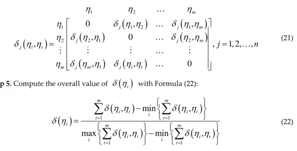
(21)Step 5. Compute the overall value of
( )
i with Formula (22):( )
(
)
(
)
(
)
(
)
1 1 1 1,
min
,
max
,
min
,
m m i t i t i t t i m m i t i t i i t t
= = = =
−
=
−
(22)Step 6. To choose the best alternative by rank the values of
( )
i , the alternative withmaximum value is the best choice.
4. The Numerical Example
4.1. Calculation Steps Based on MAGDM Problems
Construction engineering projects have the following characteristics: large investment, many participants, complex project environment, and a wide range of risk factors on the basis of the engineering procurement construction (EPC) mode. Therefore, it is necessary to analyze and assess risks during the life cycle of a construction engineering project, with a risk assessment being beneficial for implementing projects and completing project goals. Construction engineering projects face a range of political, economic, social natural and other types of risks during the implementation process. These risks have a great influence on construction companies, and produce many high probability factors which are difficult to estimate and quantify. Thus, we provide a numerical example for construction engineering project risk assessment (adapted from Reference [27]), using the TODIM method with 2TLNNs, in order to illustrate the method proposed in this paper. Assuming that there are five possible construction projects
i(
i
=
1, 2, 3, 4, 5
)
to select from and four criteria to assess theseconstruction projects: ① G1 is the construction work environment; ② G2 is the construction site safety
protection measures; ③ G3 is the safety management ability of the engineering project management; and
④ G4 is the safety production responsibility system. The five possible construction projects
(
1, 2, 3, 4, 5)
i i = are to be evaluated with 2TLNNs with the four criteria by three experts k
d (criteria weight
w
=
(
0.14, 0.33, 0.29, 0.24
)
, experts weightv
=
(
0.45, 0.15, 0.40 .
)
, listed in Tables 1–3.Table 1. 2-tuple linguistic neutrosophic numbers (2TLNNs) evaluation matrix by
d
1.G1 G2 G3 G4 1
{(s4,0), (s2,0), (s1,0)} {(s5,0), (s3,0), (s2,0)} {(s4,0), (s1,0), (s1,0)} {(s3,0), (s2,0), (s2,0)} 2
{(s5,0), (s4,0), (s4,0)} {(s3,0), (s4,0), (s2,0)} {(s2,0), (s1,0), (s3,0)} {(s4,0), (s1,0), (s2,0)} 3
{(s5,0), (s4,0), (s2,0)} {(s2,0), (s4,0), (s5,0)} {(s3,0), (s2,0), (s4,0)} {(s2,0), (s1,0), (s4,0)} 4
{(s3,0), (s2,0), (s3,0)} {(s4,0), (s3,0), (s2,0)} {(s3,0), (s3,0), (s4,0)} {(s2,0), (s1,0), (s1,0)} 5
{(s1,0), (s4,0), (s5,0)} {(s2,0), (s3,0), (s1,0)} {(s3,0), (s4,0), (s5,0)} {(s2,0), (s4,0), (s3,0)}Table 2. 2TLNNs evaluation matrix by
d
2. G1 G2 G3 G4 1
{(s5,0), (s1,0), (s2,0)} {(s4,0), (s3,0), (s1,0)} {(s4,0), (s2,0), (s1,0)} {(s5,0), (s1,0), (s2,0)} 2
{(s4,0), (s3,0), (s3,0)} {(s3,0), (s1,0), (s4,0)} {(s2,0), (s1,0), (s3,0)} {(s5,0), (s4,0), (s1,0)} 3
{(s3,0), (s4,0), (s3,0)} {(s2,0), (s4,0), (s5,0)} {(s5,0), (s1,0), (s2,0)} {(s2,0), (s1,0), (s2,0)} 4
{(s4,0), (s5,0), (s4,0)} {(s2,0), (s3,0), (s4,0)} {(s3,0), (s3,0), (s4,0)} {(s4,0), (s4,0), (s5,0)} 5
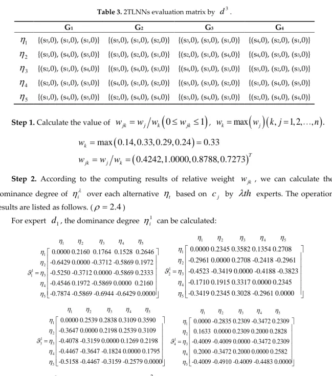
{(s2,0), (s4,0), (s5,0)} {(s3,0), (s1,0), (s5,0)} {(s2,0), (s3,0), (s4,0)} {(s2,0), (s1,0), (s3,0)}Table 3. 2TLNNs evaluation matrix by
d
3.G1 G2 G3 G4 1
{(s5,0), (s1,0), (s1,0)} {(s5,0), (s1,0), (s2,0)} {(s3,0), (s3,0), (s1,0)} {(s4,0), (s2,0), (s1,0)} 2
{(s5,0), (s4,0), (s5,0)} {(s3,0), (s2,0), (s1,0)} {(s2,0), (s1,0), (s4,0)} {(s4,0), (s5,0), (s3,0)} 3
{(s2,0), (s1,0), (s4,0)} {(s5,0), (s4,0), (s3,0)} {(s4,0), (s3,0), (s3,0)} {(s5,0), (s2,0), (s3,0)} 4
{(s2,0), (s1,0), (s3,0)} {(s4,0), (s1,0), (s2,0)} {(s5,0), (s3,0), (s2,0)} {(s1,0), (s4,0), (s5,0)} 5
{(s1,0), (s4,0), (s5,0)} {(s2,0), (s4,0), (s4,0)} {(s3,0), (s4,0), (s3,0)} {(s2,0), (s4,0), (s4,0)}Step 1. Calculate the value of
w
jk=
w w
j k(
0
w
jk
1
)
,w
k=
max
( )
w
j(
k j
,
=
1, 2,
,
n
)
.
(
)
(
)
max
0.33
0.4242,
, 0.8788, 0.7
0.14, 0.33, 0.29, 0.2
1.00
00
273
4
k T jk j kw
w
w
w
=
=
=
=
Step 2. According to the computing results of relative weight
w
jk , we can calculate the dominance degree of i
over each alternative
t based onc
j by
th
experts. The operationresults are listed as follows. (
=
2.4
)For expert
d
1, the dominance degree
i1 can be calculated:1 2 3 4 5 1 2 1 3 1 4 5 0.0000 0.2160 0.1764 0.1528 0.2646 -0.6429 0.0000 -0.3712 -0.5869 0.1972 -0.5250 -0.3712 0.0000 -0.5869 0.2333 -0.4546 0.1972 -0.5869 0.0000 0.2160 -0.7874 -0.5869 -0.6944 -0.6 = 429 0.0000 1 2 3 4 5 1 2 1 3 2 4 5 0.0000 0.2345 0.3582 0.1354 0.2708 -0.2961 0.0000 0.2708 -0.2418 -0.2961 -0.4523 -0.3419 0.0000 -0.4188 -0.3823 -0.1710 0.1915 0.3317 0.0000 0.2345 -0.3419 0.2345 0.3028 -0.296 = 1 0.0000 1 2 3 4 5 1 2 1 3 3 4 5 0.0000 0.2539 0.2838 0.3109 0.3590 -0.3647 0.0000 0.2198 0.2539 0.3109 -0.4078 -0.3159 0.0000 0.1269 0.2198 -0.4467 -0.3647 -0.1824 0.0000 0.1795 -0.5158 -0.4467 -0.3159 -0.257 = 9 0.0000 1 2 3 4 5 1 2 1 3 4 4 5 0.0000 -0.2835 0.2309 -0.3472 0.2309 0.1633 0.0000 0.2309 0.2000 0.2828 -0.4009 -0.4009 0.0000 -0.3472 0.2309 0.2000 -0.3472 0.2000 0.0000 0.2582 -0.4009 -0.4910 -0.4009 -0.448 = 3 0.0000
For expert
d
2, the dominance degree 2i
1 2 3 4 5 1 2 2 3 1 4 5 0.0000 0.1764 0.2160 0.2333 0.2646 -0.5250 0.0000 0.1247 0.1528 0.1972 -0.6429 -0.3712 0.0000 0.1528 0.1528 -0.6944 -0.4546 -0.4546 0.0000 0.1764 -0.7874 -0.5869 -0.4546 -0.525 = 0 0.0000 1 2 3 4 5 1 2 2 3 2 4 5 0.0000 0.3317 0.3582 0.3028 0.3582 -0.4188 0.0000 0.3028 0.2345 0.1354 -0.4523 -0.3823 0.0000 -0.2418 -0.3419 -0.3823 -0.2961 0.1915 0.0000 0.2708 -0.4523 -0.1710 0.2708 0.2708 = 0.0000 1 2 3 4 5 1 2 2 3 3 4 5 0.0000 0.2838 -0.3159 0.2838 0.3109 -0.4078 0.0000 -0.3647 0.2539 0.2198 0.2198 0.2539 0.0000 0.3109 0.3358 -0.4078 -0.3647 -0.4467 0.0000 0.1269 -0.4467 -0.3159 -0.4825 -0.182 = 4 0.0000 1 2 3 4 5 1 2 2 3 4 4 5 0.0000 0.2309 0.2000 0.3055 0.2309 -0.4009 0.0000 0.3055 0.2582 0.3266 -0.3472 -0.5304 0.0000 0.3266 0.1155 -0.5304 -0.4483 -0.5670 0.0000 -0.5304 -0.4009 -0.5670 -0.2005 0.305 = 5 0.0000
For expert
d
3, the dominance degree
i3 can be calculated:1 2 3 4 5 1 2 3 3 1 4 5 0.0000 0.2333 0.2160 0.1972 0.2925 -0.6944 0.0000 -0.6944 -0.7424 0.1764 -0.6429 0.2333 0.0000 -0.2625 0.1972 -0.5869 0.2494 0.0882 0.0000 0.2160 -0.8705 -0.5250 -0.5869 -0.642
= 9 0.0000 1 2 3 4 5 1 2 3 3 2 4 5 0.0000 0.2708 0.2708 0.1354 0.3830 -0.3419 0.0000 0.3317 -0.2961 0.3317 -0.3419 -0.4188 0.0000 -0.3823 0.2708 -0.1710 0.2345 0.3028 0.0000 0.3582 -0.4835 -0.4188 -0.3419 -0.452 = 3 0.0000 1 2 3 4 5 1 2 3 3 3 4 5 0.0000 0.3109 0.2198 -0.3159 0.2198 -0.4467 0.0000 -0.4078 -0.4825 0.2838 -0.3159 0.2838 0.0000 -0.2579 0.1795 0.2198 0.3358 0.1795 0.0000 0.2539 -0.3159 -0.4078 -0.2579 -0.364 = 7 0.0000 1 2 3 4 5 1 2 3 3 4 4 5 0.0000 0.2582 0.2000 0.3464 0.3055 -0.4483 0.0000 -0.4009 0.2828 0.2309 -0.3472 0.2309 0.0000 0.3266 0.2828 -0.6014 -0.4910 -0.5670 0.0000 -0.2835 -0.5304 -0.4009 -0.4910 0.163
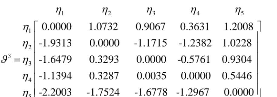
= 3 0.0000 Step 3. Compute overall dominance degree j j
(
i,
t)
m m
=
to get the matrix(
i,
t)
m m
=
. 1 2 3 4 5 1 2 1 3 4 50.0000
0.4209
1.0494
0.2518
1.1253
-1.1405
0.0000
0.3504 -0.3748
0.4948
-1.7860
-1.4299
0.0000 -1.2260
0.3018
-0.8723
-0.3233
-0.2376
0.0000
0.8882
-2.0461
-1.2902
-1.1085 -1.64
=
52
0.0000
1 2 3 4 5 1 2 2 3 4 50.0000
1.0228 0.4584
1.1254 1.1647
-1.7524 0.0000 0.3683 0.8993 0.8791
-1.2226 -1.0300 0.0000 0.5485 0.2621
-2.0149
-1.5637 -1.2769 0.0000 0.0437
-2.0874
-1.6408 -0.8
=
668 -0.1310
0.0000
1 2 3 4 5 1 2 3 3 4 5
0.0000
1.0732
0.9067
0.3631
1.2008
-1.9313
0.0000
-1.1715 -1.2382 1.0228
-1.6479
0.3293
0.0000 -0.5761 0.9304
-1.1394
0.3287
0.0035 0.0000 0.5446
-2.2003
-1.7524
-1.67
=
78 -1.2967
0.0000
Step 4. Calculate the overall dominance
(
i,
t)
based on the expert weighting vector(
0.45, 0.15, 0.40
)
and the results of(
i,
t)
m m
=
.(
)
1 2 3 4 5 1 2 3 4 50.0000
0.7721
0.9037
0.4274
1.1614
-1.5486
0.0000
-0.2557
-0.5290
0.7637
,
-1.6463
-0.6662
0.0000
-0.6998
0.5473
-1.1505
-0.2485
-0.2971
0.0000
0.6241
-2.1140
-1.5277
-i t
=
1.3000
-1.2787
0.0000
Step 5. Compute the overall value of
( )
i with the Formula (22):( )
11.0000
,
( )
20.4903
,
( )
30.3959
,
( )
40.5428
,
( )
50.000
0
.
=
=
=
=
=
Step 6. To choose the best alternative by rank the values of
( )
i , the alternative with maximum value is the best choice. According to step 5, the ranking of
i is
1
4
2
3
5, and it is clear that the best choice is
1.4.2. The Affection Analysis of the Parameter
By altering parameters
in the computing process of the 2TLNNs TODIM method, we can depict the effects on ordering. The calculation results follow.From the calculation results of Table 4, we can easily ascertain that the best alternative is
1 by altering the values of
. Next we will compare our proposed 2TLNNs TODIM method with the existing method using 2TLNNWA and 2TLNNWG operators.Table 4. Ordering of