Nonlinear Cointegration Analysis and the Environmental Kuznets Curve

(1)

IHS Economics Series

Working Paper 224

July 2008

Nonlinear Cointegration Analysis and

the Environmental Kuznets Curve

Seung Hyun Hong

Martin Wagner

(2)

Impressum Author(s):

Seung Hyun Hong, Martin Wagner

Title:

Nonlinear Cointegration Analysis and the Environmental Kuznets Curve

ISSN: Unspecified

2008 Institut für Höhere Studien - Institute for Advanced Studies (IHS)

Josefstädter Straße 39, A-1080 Wien

E-Mail: o ce@ihs.ac.atﬃ

Web: www .ihs.ac. a t

All IHS Working Papers are available online: http://irihs. ihs. ac.at/view/ihs_series/

(3)

Nonlinear Cointegration

Analysis and the

Environmental Kuznets Curve

Seung Hyun Hong, Martin Wagner

224 Reihe Ökonomie

Economics Series

(4)

(5)

224 Reihe Ökonomie

Economics Series

Nonlinear Cointegration

Analysis and the

Environmental Kuznets Curve

Seung Hyun Hong, Martin Wagner

July 2008

Institut für Höhere Studien (IHS), Wien

Institute for Advanced Studies, Vienna

(6)

Contact:

Seung Hyun Hong Department of Economics Concordia University 1455 de Maisonneuve Blvd. West Montreal, Quebec H3G 1M8 email: shhong@alcor.concordia.ca Martin Wagner

Department of Economics and Finance Institute for Advanced Studies Stumpgergasse 56

1060 Vienna, Austria

: +43/1/599 91-150

email: Martin.Wagner@ihs.ac.at

Founded in 1963 by two prominent Austrians living in exile – the sociologist Paul F. Lazarsfeld and the economist Oskar Morgenstern – with the financial support from the Ford Foundation, the Austrian Federal Ministry of Education and the City of Vienna, the Institute for Advanced Studies (IHS) is the first institution for postgraduate education and research in economics and the social sciences in Austria. The Economics Series presents research done at the Department of Economics and Finance and aims to share “work in progress” in a timely way before formal publication. As usual, authors bear full responsibility for the content of their contributions.

Das Institut für Höhere Studien (IHS) wurde im Jahr 1963 von zwei prominenten Exilösterreichern – dem Soziologen Paul F. Lazarsfeld und dem Ökonomen Oskar Morgenstern – mit Hilfe der Ford-Stiftung, des Österreichischen Bundesministeriums für Unterricht und der Stadt Wien gegründet und ist somit die erste nachuniversitäre Lehr- und Forschungsstätte für die Sozial- und Wirtschafts-wissenschaften in Österreich. Die Reihe Ökonomie bietet Einblick in die Forschungsarbeit der Abteilung für Ökonomie und Finanzwirtschaft und verfolgt das Ziel, abteilungsinterne Diskussionsbeiträge einer breiteren fachinternen Öffentlichkeit zugänglich zu machen. Die inhaltliche Verantwortung für die veröffentlichten Beiträge liegt bei den Autoren und Autorinnen.

(7)

Abstract

Recent years have seen a growing literature on the environmental Kuznets curve (EKC) that resorts in a large part to cointegration techniques. The EKC literature has failed to acknowledge that such regressions involve unit root nonstationary regressors and their integer powers (e.g. GDP and GDP squared), which behave differently from linear cointegrating regressions. Here we provide the necessary tools for EKC analysis by deriving estimation and testing theory for cointegrating equations including stationary regressors, deterministic regressors, unit root nonstationary regressors and their integer powers. We consider fully modified OLS estimation, specification tests based on augmented and auxiliary regressions, as well as a sub-sample KPSS type cointegration test. We present simulation results illustrating the performance of the estimators and tests. In the empirical application for CO2 and SO2 emissions for 19 early industrialized countries over the period 1870-2000

we find evidence for an EKC in roughly half of the countries.

Keywords

Integrated Process, Nonlinear Transformation, Fully Modified Estimation, Nonlinear Cointegration Analysis, Environmental Kuznets Curve

JEL Classification

C12, C13, Q20

(8)

(9)

1 Introduction

1 2 Econometric

Theory

3

2.1 Setup and Assumptions ... 3

2.2 OLS Estimation... 7

2.3 Fully Modified OLS Estimation... 8

2.4 Specification Testing based on Augmented and Auxiliary Regressions... 10

2.5 KPSS Type Tests for Cointegration... 14

3 Simulation

Performance

18

3.1 Performance of the Estimators ... 18

3.2 Performance of the Augmented and Auxiliary Regression Tests ... 19

3.3 Performance of the KPSS Type Tests... 25

4 Environmental Kuznets Curves

26

5 Summary and Conclusions

36 References 38

Appendix A: Proofs

42

(10)

(11)

1 Introduction

Since the seminal work of Grossmann and Krueger (1993, 1995) many econometric studies of the relationship between measures of economic development (typically proxied by per capita GDP) and pollution, respectively emissions, have been conducted. Survey articles like Stern (2004) or Yandle, Bjattarai, and Vijayaraghavan (2004) count more than one-hundred refereed publications. Most of the papers focus on a specific conjecture, the so called ‘environmental Kuznets curve’ (EKC) hypothesis, which postulates an inverted U-shaped relationship between the level of economic de-velopment and the degree of income inequality. The term EKC refers by analogy to the inverted U-shaped relationship between the level of economic development and the degree of income in-equality postulated by Kuznets (1955) in his 1954 presidential address to the American Economic Association.

The largest part of the empirical EKC literature estimates parametric EKCs, however, also other estimation strategies have been followed in the empirical EKC literature: non-parametric EKCs (see e.g. Millimet, List, and Stengos, 2003), semi-parametric EKCs (see e.g. Bertinelli and Strobl, 2005) or EKCs using spline interpolations (see e.g. Schmalensee, Stoker, and Judson, 1998). Within the parametric EKC literature many studies rely upon unit root and cointegration analysis given the widespread non-rejection of the unit root hypothesis for GDP. With the exception of very few papers who note and bypass in one way or another the associated problems (see Bradford, Fender, Shore, and Wagner, 2005; M¨uller-F¨urstenberger and Wagner, 2007; Wagner, 2008), the empirical EKC literature fails to acknowledge the implications of the presence of nonlinear transformations of unit root processes. In a typical EKC, compare (19) below, emissions are regressed on GDP and GDP squared. Since (log per capita) GDP is often well characterized as being a unit root process, GDP squared is a nonlinear transformation of an integrated process and regressions involving such processes require different asymptotic theory than the usual ‘linear’ unit root and cointegration analysis.

In this paper we derive the asymptotic distributions of both the OLS estimator as well as of a fully modifiedOLS (FM-OLS) estimator of equations containing deterministic variables, stationary regressors, integrated regressors and integer powers of integrated regressors. The results we obtain resemble in several respects that of linear cointegration analysis as derived in Phillips and Hansen (1990) and rely upon the important contributions of Chang, Park, and Phillips (2001) and Park and Phillips (1999, 2001). First, the OLS estimator is consistent, but its limiting distribution is

(12)

contaminated by so called second order bias terms, rendering valid inference infeasible. Second, the proposed FM-OLS estimator has a limiting distribution that is free of second order biases and thus forms the basis for asymptotically valid χ2_{-inference for certain hypotheses. Third, this property}

of the limiting distribution of the FM-OLS estimator also forms the basis for specification testing based on augmented respectively auxiliary regressions including higher order polynomial powers of the integrated regressors and/or polynomial powers of additional integrated regressors. In this re-spect we consider tests based on both the Wald and Lagrange Multiplier testing principles. Fourth, we consider a KPSS type (compare Kwiatkowski, Phillips, Schmidt, and Shin, 1992) cointegration test to directly test the null hypothesis of nonlinear cointegration for a given specification. Since the asymptotic distribution of this test is contaminated by nuisance parameters we follow Choi and Saikkonen (2005) and present a sub-sample version of the test that has an asymptotic distribution free of nuisance parameters. Since the sub-sample test can be used in conjunction with the Bonfer-roni bound we investigate the potential performance gains that can be realized by using adjusted Bonferroni bound test procedures that are less conservative, such as those proposed in Simes (1986) or Rom (1990).

We conduct a small simulation study to assess the performance of the proposed methods. The findings show that the FM-OLS correction has only modest effects on the biases of the coefficients estimated by FM-OLS compared to the – also consistent – OLS estimates. The effects are much larger on the tests, whose performance hinges crucially on applying appropriate FM-OLS correc-tions. The Wald and Lagrange Multiplier tests behave very similarly and perform very well in terms of size. Their power performance depends, as expected, quite strongly upon the auxiliary regressors as well as the alternative considered. With respect to the sub-sample KPSS type tests we note that all considered modifications of the Bonferroni bound lead to very similar performance in the simulations. The KPSS type tests tend to be undersized for small samples and their power increases quite slowly with the sample size. However, their power is quite similar for all considered alternatives, which is consistent with the fact that the KPSS type tests are not specified against any particular alternative.

After the simulations we turn to the empirical analysis where we study the relationship between CO2 respectively SO2 emissions and GDP for a panel of 19 early developed countries over the

period 1870–2000. When considering a quadratic formulation of the EKC we find support, based on the LM specification test, for eight countries for CO2 emissions and for five countries SO2

(13)

nonlinear cointegrating relationship in three more countries for both CO2 and SO2 emissions. The

turning points implied by the FM-OLS coefficient estimates are with very few exceptions reasonable in-sample values.

The paper is organized as follows. In Section 2 we derive the asymptotic results for the estimators and tests. Section 3 contains a small simulation study to assess the finite sample performance of the proposed methods and Section 4 contains the results of the EKC analysis. Section 5 briefly summarizes and concludes. Two appendices follow the main text: Appendix A contains the proofs of all propositions results and Appendix B collects additional material related to the empirical EKC analysis.

We use the following notation: As usual, the symbols ⇒ and →p signify weak convergence

and convergence in probability, respectively. Definitional equality is signified by :=. Further, aT =O(Tn) (respectivelyaT =Op(Tn)) denotes that{aT} is at most of orderTn (in probability).

Standard Brownian motions are denoted as W(r) or in short W, whereas Brownian motions with non-identity covariance matrices (specified in the context) are denoted withB(r) orB. For integrals of the formR₀1B(s)dsandR₀1B(s)dB(s) we use short-hand notationR BandRBdB. For notational simplicity we also often drop function arguments. Withbxcwe denote the integer part ofx∈Rand diag(·) denotes a diagonal matrix with the entries specified throughout. E denotes the expected value andL denotes the backward-shift operator, i.e. L{xt}t∈Z={xt−1}t∈Z.

2 Econometric Theory

2.1 Setup and Assumptions

We consider the following equation including stationary regressors wit, i = 1, . . . , n, a constant,

polynomial time trends up to powerq and integer powers of integrated regressors xjt, j = 1, . . . , m

up to degreesp_j yt=w0tθw+Dt0θD+ m X j=1 X_jt0 θXj+ut , fort= 1, . . . , T (1) with wt := [w1t, . . . , wnt]0, Dt := [1, t, t2, . . . , tq]0, xt := [x1t, . . . , xmt]0, Xjt := [xjt, x2jt, . . . , xpjjt]0

and the parameter vectors θD ∈ Rq+1, θw ∈ Rn and θXj ∈ Rpj. Furthermore define for later use

X_t:= [X0

1t, . . . , Xmt0 ]0,Zt:= [wt0, D0t, Xt0]0 and p:=

P_m

(14)

In a more compact way,

y = wθw+DθD+XθX +u (2)

= Zθ+u,

withy:= [y1, . . . , yT]0,u:= [u1, . . . , uT]0,Z := [w D X] and θ= [θw0 θD0 θ0X]0 ∈R(q+1)+n+p and

w:=    w0 1 .. . w0 T   ∈RT×n, D:=    D0 1 .. . D0 T   ∈RT×(q+1), X :=    X0 1 .. . X0 T   ∈RT×p.

Let us next state the assumptions concerning the regressors and the error processes:

Assumption 1 The processes {∆xt}t∈Z, {wt}t∈Z and {ut}t∈Z are generated as

∆xt=vt = Cv(L)εt= ∞ X j=0 cvjεt−j wt = Cw(L)ηt= ∞ X j=0 cwjηt−j ut = Cu(L)ζt= ∞ X j=0 cujζt−j,

with the summability conditions

Cv(1)6= 0, ∞ X j=0 j||cvj||<∞, ∞ X j=0 j1/2||cwj||<∞, ∞ X j=0 j1/2|cuj|<∞.

Furthermore we assume that the regressors are predetermined, i.e. we assume that the process

{ξ_t0}t∈Z ={[ε0t+1, ηt0+1, ζt]0}t∈Z is a stationary and ergodic martingale difference sequence with

na-tural filtration Ft=σ ³© ξ0 s ª_t −∞ ´

and denote the (conditional) covariance matrix by

Σ0 =   Σεε Σεη Σεζ Σ_ηε Σ_ηη Σ_ηζ Σζε Σζη σζ2  _:=_E₍_ξ0 t(ξt0)0|Ft−1).

We also assume that Σww:=Ewtwt0 >0.

The above assumptions allow to draw on the asymptotic results of Chang, Park, and Phillips (2001) and Park and Phillips (1999, 2001). The assumption that the regressors are predetermined implies that the conditional expectation E(y_t|F_t₋₁) = 0, which is usual in nonlinear regression theory. Considering the stationary regressors to have zero mean is only done for convenience and

(15)

is not a restriction since typically an intercept will be included in a regression. The assumption C_v(1)6= 0 implies that x_t is indeed an integrated process whereas Σ_ww >0 is mainly put in place for convenience as it is likely to be fulfilled in all practical applications.

Further additionally required moment assumptions given below are also similar to those formu-lated in Chang, Park, and Phillips (2001).

Assumption 2 For the process {ξ0

t}t∈Z the following conditions hold:

1. sup_t_≥₁E(kξ0

tkr|Ft−1)<∞a.s. for some r >4.

2. E

³

(ξ0

i,t)2ξ0j,t−l

´

= 0 for all i, j and for all l≥1.

3. ζt is i.i.d. with E(|ζ|r) < ∞ for some r > 8 and its distribution function is absolutely

continuous with respect to the Lebesgue measure and for the characteristic functionϕit holds thatϕ(λ) =o(|λ|−δ₎ _as _λ_{→ ∞} _{for some} _{δ >}₀_.

The above assumptions are sufficient for the following invariance principle to hold for {ξ_t}_t_∈_Z=

{[v0

t+1, wt0+1, ut]0}t∈Z using the Beveridge-Nelson decomposition (compare Phillips and Solo, 1992)

1 √ T [T r] X t=1 ξt⇒B(r) =   _BB_wv(₍r_r)₎ Bu(r)  _. ₍₃₎

Note here that it holds thatB(r) = Ω1/2W(r) with the long-run covariance matrix Ω :=P∞_h₌_−∞E(ξ0ξh0).

We also define the one-sided long-run covariance Λ :=P∞_h₌₀E(ξ0ξ_h0) and both covariance matrices

are partitioned according to the partitioning ofξt, i.e.:

Ω =   _ΩΩ_wvvv _ΩΩ_wwvw _ΩΩ_wuvu Ωuv Ωuw ωuu   _, _{Λ =}   _ΛΛ_wvvv _ΛΛ_wwvw _ΛΛ_wuvu Λuv Λuw λuu  _.

When referring to quantities corresponding to only one of the nonstationary regressors and its powers, e.g. Xjt, we use the according notation, e.g. Bvj(r) or Λvju.

To study the asymptotic behavior of the estimators, we next introduce appropriate weighting matrices, whose entries reflect the divergence rates of the corresponding variables. Thus, denote with G(T) =diag{Gw(T), GD(T), GX(T)}, where for notational brevity we often use G:=G(T).

(16)

The three diagonal sub-matrices are given by: G_w(T) :=    T−1/2 . .. T−1/2   ∈Rn×n, G_D(T) :=    T−1/2 . .. T−(q+1/2)   ∈R(q+1)×(q+1), GX(T) :=    GX1 . .. GXm   ∈Rp×p withGXj :=    T−1 . .. T−pj₂+1   ∈Rpj×pj.

Using these weighting matrices, we can define the following limits of the major building blocks. For tsuch that limT→∞t/T =r the following results hold:

lim T→∞ √ T GD(T)Dt = lim T→∞    1 . .. T−q       1 .. . tq   =    1 .. . rq   =:D(r) lim T→∞ √ T GXj(T)Xjt = lim T→∞    T−1/2 . .. T−pj/2       xjt .. . xpj_jt   =    Bvj .. . Bvjpj   =:Bvj(r),

separating here the coordinates of vt = [v1t, . . . , vmt]0 corresponding to the different variables

x_jt. The first result is immediate and the second follows from Chang, Park, and Phillips (2001, Lemma 5). The stacked vector of the scaled polynomial transformations of the integrated processes is denoted as Bv(r) := [Bv1(r)0, . . . ,Bvm(r)0]0. We are confident that D as defined in (2) is not

confused withD(r) defined above even when the latter is used in abbreviated form Din integrals.

Remark 1 More general deterministic components can be included with the necessary condition being that the correspondingly defined limit quantity satisfies RDD0 _> ₀_{, i.e. that the considered}

functions are linearly independent in L2_[0_,_1]_{. This allows in addition to the polynomial trends on}

which we focus in this paper e.g. also to include time dummies, broken trends or trigonometric functions of time (compare the discussion in Park, 1992).

The relationship postulated in (1) is restrictive in the sense that e.g. no cross-products of the formxm_itxn_jt ortmxn_jt are included. Considering such cross-terms increases not only the flexibility of the functional form but also immediately allows for an interpretation of the estimated relationship as a Taylor expansion of an unknown nonlinear function. The theory developed in this paper, based on the underlying results of Park and Phillips (1999, 2001), can be extended to include these cross-terms. However, the curse of dimensionality will often limit the practical usefulness of

(17)

specifications including all cross-terms. Also for the empirical application in this paper we consider only one integrated regressor, namely per capita GDP.

2.2 OLS Estimation

We first study the asymptotic behavior of the OLS estimator. As in the linear cointegration case, its limiting distribution is contaminated by nuisance parameters due to serial correlation in the error process{ut}t∈Z and endogeneity of{∆Xt}t∈Z. Both of these aspects are very similar to those

in the linear case as in Phillips and Hansen (1990) and are summarized in Proposition 1.

Proposition 1 Let yt be generated from (1) with the regressors Zt and errors ut satisfying

As-sumptions 1 and 2. Then the asymptotic distribution of the OLS estimator θˆ := (Z0_Z₎−1_Z0_y _is

given by G−1(ˆθ−θ) =   G−1 w (ˆθw−θw) G−_D1(ˆθD −θD) G−_X1(ˆθ_X −θ_X)   ⇒     Σ−1 wwNwu hR ˜ DD˜0 i₋₁_nR ˜ DdBu− R DB0_v£RBvB0v ¤₋₁ M o hR _˜ BvB˜0v i₋₁_nR ˜ BvdBu.v− R _˜ BvdBv0Ω−vv1Ωvu+M o     (4) where B_u.v(r) := B_u(r)−Ω_uvΩ−1

vvBv(r) with corresponding variance ωu.v := ωu −ΩuvΩ−vv1Ωvu

and Nwu := limT→∞√1_T

P_T

t=1wtut. The random variable Nwu is normally distributed with mean

Σwu := E(wtut) and variance depending upon the coefficients cw,j, cu,j, Σηη and σ2_ζ given in

As-sumption 1. Furthermore ˜ D := D− Z DB0_v µZ B_vB0_v ¶₋₁ B_v, ˜ Bv := Bv− Z BvD0 µZ DD0 ¶₋₁ D, and M :=    M1 .. . Mm    where Mj := Λvju      1 2R Bvj(r)dr .. . pj R Bvj(r)pj−1dr     . (5)

The limiting distribution of the consistent OLS estimator displayed in (4) is contaminated by so-calledsecond orderbias terms: the serial correlation bias and the endogeneity bias, using the same

(18)

names in our nonlinear setup as used in the limiting distribution of the OLS estimator in the linear cointegration case (see Phillips and Hansen, 1990). Note that whenX_t is strictly exogenous, these bias terms vanish with Λvu= Ωvu= 0. If this is not the case, standard inference on the parameters

becomes invalid due to the presence of these bias terms.

Remark 2 Note that the serial correlation bias term M, which is due to correlation between ut

and v_t, appears not only in the limiting distribution of θˆ_X, but also in that of θˆ_D, reflecting the asymptotic correlation between deterministic and stochastic trends. Thus, putting these two blocks of the coefficient vectorθtogether inθN :=

£

θ0

D θX0

¤₀

, we can explicitly identify the source of the serial correlation bias by writing the limiting distribution of the OLS estimator of θD as

G−_N1 ³ ˆ θ_N −θ_N ´ ⇒ µZ JJ0 ¶₋₁½Z JdBu+ µ 0₍_q₊₁₎_×₁ M ¶¾ , for J(r) :=£ D(r)0 _B v(r)0 ¤₀ andGN :=diag(GD, GX).

2.3 Fully Modified OLS Estimation

Two ways to remove the bias terms present in the OLS limiting distributions have been proposed in the cointegration literature. These are fully modified OLS (FM-OLS) estimation (see Phillips and Hansen, 1990) based on a direct non-parametric correction and dynamic OLS (D-OLS) esti-mation (see Saikkonen, 1991) where the correction is achieved by running lead and lag augmented regressions. In this paper we consider FM-OLS estimation which requires consistent estimators of the bias terms. In this respect define

M∗ :=    M∗ 1 .. . M∗ m    , M_j∗ := ˆΛ+_vju      T 2Pxjt .. . p_jPxpj_jt−1     , (6)

with a consistent estimator ˆΛ+

vju:= ˆΛvju−ΩˆuvΩˆ−vv1Λˆvvj. Once appropriately scaled the quantityM∗

in (6) converges to M as given in (5), which in conjunction with using the transformed dependent variable1 y+_t :=yt−ΩˆuvΩˆvv−1vt,y+ := [y1+, . . . , y+T]0 leads to an asymptotic distribution that is free

of bias terms as summarized in the following Proposition 2.

1_{For notational simplicity we ignore the dependence of} _y+ _{upon the specific consistent long-run covariance} esti-mator chosen.

(19)

Proposition 2 Let y_t be generated by (1) with the regressorsZ_t and errors u_t satisfying Assump-tions 1 and 2. Define the FM-OLS estimator of θ as

ˆ θ+:= (Z0Z)−1¡Z0y+−A∗¢, with A∗ :=   ˆ Σ+ wu 0₍_q₊₁₎_×₁ M∗   withΣˆ+

wua consistent estimator ofΣ+wu:= Σwu−ΣwvΩvv−1ΩvuandM∗ as given in(6)with consistent

estimators of the required long-run (co)variances. Then the asymptotic distribution of θˆ+ is given by G−1 ³ ˆ θ+−θ ´ =   G−1 w (ˆθw+−θw) G−_D1(ˆθ_D+−θD) G−_X1(ˆθ+_X−θX)  _⇒     Σ−1 wwNwu.v hR ˜ DD˜0 i₋₁_R ˜ DdBu.v hR _˜ BvB˜0v i₋₁_R ˜ BvdBu.v    , (7)

with a normally distributed mean zero random variable N_wu.v := lim_T_→∞ _√1

T

P_T

t=1wtu+t , where

u+_t :=ut−ΩˆuvΩˆ−vv1vt.

Using the quantities defined in Remark 2 it holds more compactly written thatG−_N1

³ ˆ θ_N+−θN ´ ⇒ ¡R JJ0¢−1R_JdB

u.v. The limiting distribution of G−_N1(ˆθ+_N −θN) is free of second order bias terms

and mixed normal with mean zero. This stems from the fact that the vector ˜Bv is, by construction,

independent ofB_u.v.

As shown in Phillips and Hansen (1990, Theorem 5.1) the special form of the FM-OLS limiting distribution allows for asymptotic χ2_{-inference for testing} _certain _{linear hypothesis on the}

coef-ficients by using the Wald test. From the discussion in Phillips and Hansen (1990, p. 106), in particular from the corresponding proofs in their paper, it becomes clear that only certain linear hypotheses can be tested with asymptotic χ2_{-inference. A similar result that allows to test for}

certain hypotheses, which we formulate for notational convenience forθN as defined in Remark 2,

can be established in our setup.

Proposition 3 Let yt be generated by (1) with the regressorsZt and errors ut satisfying

Assump-tions 1 and 2. Consider s linearly independent restrictions collected in

(20)

withR∈Rs×q+1+p _{with full rank}_s_and_r _∈_Rs_{. Furthermore let}_ω_ˆ

u.v denote a consistent estimator

of ωu.v. Then it holds with ZN = [D X]that the Wald statistic

W := ³ Rθˆ_N+−r ´₀h ˆ ωu.vR ¡ Z_N0 ZN ¢₋₁ R0 i₋₁³ Rθˆ+_N −r ´ (8) is under the null hypothesis asymptotically distributed as χ2

s under one of the following conditions:

(i) H0 only involves coefficients with the same convergence rate, or

(ii) each of the restrictions in H0 involves only one coefficient, i.e. the off-diagonal elements of

R are all equal to 0.

The above result implies that for instance the appropriate t-statistic for coefficientθi, withθi a

component of θN, given by tθi :=

ˆ θ+ i q ˆ ωu.v(Z0_Z₎−1 [i,i]

, is asymptotically standard normally distributed. Note furthermore that hypothesis testing for the coefficients θw can simply be based on their

asymptotic normal distribution.

2.4 Specification Testing based on Augmented and Auxiliary Regressions

Testing the correct specification of equation (1) is clearly an important issue. In this respect we are particularly interested in the prevalence of cointegration, i.e. stationarity of ut. Absence

of cointegration can be due to several reasons. First, there is no cointegrating relationship of any functional form betweeny_tandx_t. Second,y_tandx_tare nonlinearly cointegrated but the functional relationship is different than postulated by equation (1). This case covers the possibilities of missing higher order polynomial terms or cointegration with a different functional form of the relationship. Third, the absence of cointegration is due to missing explanatory variables in equation (1).

In a general formulation all the above possibilities can be cast into a testing problem within the augmented regression

yt=Zt0θ+F(xt, qt, θF) +φt, (9)

whereFis such thatF(x_t, g_t,0) = 0 andq_tdenotes additional integrated regressors. If cointegration prevails in (1) thenθ_F = 0 and φt=ut.

In many cases the researcher will not have a specific parametric formulation in mind for the function F(·), which implies that typically the unknown F(·) is replaced by a partial sum ap-proximation. This approach has a long tradition in specification testing in a stationary setup, see

(21)

Ramsey (1969), Phillips (1983), Lee, White, and Granger (1993) or de Benedictis and Giles (1998). Given our FM-OLS results it appears convenient to replace the unknownF(·) by using polynomial powers of the integrated regressors, which will include higher order powers larger than pj for the

componentsxjt of xt and powers larger equal than 1 for the additional integrated regressors qit.

Of course this simple approach is also subject to the discussion in the introduction in that no multivariate expansion is considered. However, for specification analysis the advantage of a parsi-monious setup may outweigh the potential disadvantages of considering only univariate polynomials since a test based on such a formulation will also have power against alternatives where e.g. prod-ucts terms are present. Clearly, the power properties of tests based on univariate polynomials depend upon the unknown alternative F(·) and will be the more favorable the more F(·) ‘resem-bles’ univariate polynomials. This trade-off is exactly the same as in the stationary case, as also discussed in Hong and Phillips (2008).

Denote with ¯Xjt := [xpjjt+1, x pj+2 jt , . . . , x pj+rj jt ]0 for j = 1, . . . , m, Qit := [q1it, q2it, . . . , qitsi]0 for i = 1, . . . , k, F_t := [ ¯X0

1t, . . . ,X¯mt0 , Q01t, . . . , Q0kt]0 and F := [F10, . . . , FT0]0. Using this notation the

augmented polynomial regression including higher order polynomial powers of the regressors xjt

and polynomial powers of additional integrated regressorsqit can be written as

y=Zθ+F θF +φ, (10)

with φ:= [φ₁, . . . , φ_T]0_{. If equation (10) is well specified the parameters can be estimated}

consis-tently by FM-OLS according to Proposition 2 if the additional regressors qit fulfill the necessary

assumptions stated in Section 2.1 which are now modified to accommodate additional regressors.

Assumption 3 When considering additional regressors qit and their polynomial powers define

˜

v_t := [v0

t,(vt∗)0]0 = [∆x0t,∆qt0]0, with vt∗ = ∆qt and qt = [q1t, . . . , qkt]0. Assumptions 1 and 2 are

extended such that they are fulfilled for the extended process v˜t generated by C˜v(L)˜εt, with C˜v(L)

and ε˜t also extended accordingly.

Note that equation (10) can be well-specified for different reasons. The first is that (1) is a cointegrating relationship, in which case consistently estimated coefficients ˆθ_F+ will converge to their true value equal to 0. The second possibility is that (1) is misspecified, but the extended equation (10) is well-specified. In this case at least some entries of ˆθ+_F will converge to their non-zero true values. In case that (10) and consequently also (1) are misspecified andφtis not stationary,

(22)

spurious regression results similar to the linear case that lead to non-zero limit coefficients apply. Consequently, a specification test based on H₀ : θ_F = 0 is consistent against the three discussed forms of misspecification of (1) discussed in the beginning of the sub-section.

Testing the restriction θF = 0 in (10) can be done in several ways. One is given by

FM-OLS estimation of the augmented regression (10) and performing a Wald test on the estimated coefficients using Proposition 3. Another possibility is to use the FM-OLS residuals of the original equation (2) and to perform a Lagrange Multiplier RESET type test in an auxiliary regression. These two possibilities are discussed in turn.

Proposition 4 Let yt be generated by (1) with the regressors Zt, Qt and errors ut satisfying

Assumptions 1, 2 and 3. Denote with θˆ_F+ the FM-OLS estimator of θF in equation (10), with

˜

FN =F−ZN(ZN0 ZN)−1ZN0 F, and as above ZN = [D X] and let ωˆu.˜v be a consistent estimator of

ω_u._v_˜. Then it holds that the Wald test statistic for the null hypothesis H₀ :θ_F = 0 in equation (10), given by TW := ³ ˆ θ+_F ´₀³ ˜ F0 NF˜N ´ ˆ θ+_F ˆ ω_u._˜_v , (11)

is under the null hypothesis asymptotically distributed asχ2

b, withb:=

P_m

j=1rj+

P_n

j=1sj.

Note that the required variance and covariance estimates in Proposition 4 are all based on the (m+k)-dimensional process ˜v_t. The result given in Proposition 4 follows straightforwardly from Propositions 2 and 3.

The basis of the Lagrange Multiplier (LM) test are the FM-OLS residuals ˆu+_t of (2), which are regressed on ˜F in the auxiliary regression

ˆ

u+= ˜F θ_F˜ +ψt. (12)

with ˆu+ _{= [ˆ}_u+

1, . . . ,uˆ+T]0. Clearly, to allow for asymptotic standard inference the coefficients θF˜

have to be estimated by FM-OLS to achieve a second order bias free limiting distribution, since the limiting distribution of the OLS estimator of θ_F˜ in (12) also depends upon second order bias

terms (see the proof of Proposition 5 in Appendix A for details). The FM-OLS estimator as well as the test statistic for testing the hypothesisθ_F˜ = 0 are presented in the following proposition for

the case that (1) is well specified. Consistency of the tests against the above-discussed forms of misspecification of (1) follows from the same arguments as for the Wald test.

(23)

Proposition 5 Let y_t be generated by (1) with the regressors Z_t, Q_t and errors u_t satisfying As-sumptions 1, 2 and 3. Define the fully modified OLS estimator of θ_F˜ in equation (12) as

ˆ θ+_˜ F := ³ ˜ F0F˜ ´₋₁³ ˜ F0uˆ+−OF∗−MF∗+kF∗M∗ ´ , (13) with OF∗ := ˆΩu˜vΩˆ−˜v˜v1 X Ftv˜t−ΩˆuvΩˆ−vv1 X Ftvt and MF∗ _{:= [}_M0 ¯ X1, . . . , M 0 ¯ Xm, MQ0 1, . . . , M 0 Qk]0, where M_Xj¯ = ˆΛ+_vju    (p_j + 1)Pxpj_jt .. . (pj+rj) P xpj_jt+rj−1   , M_Qi = ˆΛ+_v∗ iu      T 2Pqit .. . si P q_itsi−1     , kF∗ ₌_F0_X˜_{( ˜}_X0_X˜₎−1_, _X˜ ₌_X₋_D₍_D0_D₎−1_D0_X_, _Λˆ+

vju as defined above Proposition 2 and Λˆ+v∗

iu := ˆ Λv∗ iu−ΩˆuvΩˆ −1 vvΛˆvv∗

i. Let ωˆu,˜v denote a consistent estimator ofωu,˜v. Then it holds that the LM test

statistic for the null hypothesis H0 :θ_F˜ = 0 in (12)

TLM := ³ ˆ θ+_F_˜ ´₀³ ˜ F0F˜ ´ ˆ θ_F+_˜ ˆ ωu.v˜ , (14)

is under the null hypothesis asymptotically distributed asχ2

b, withb=

P_m

j=1rj+

P_k

j=1sj.

Remark 3 Proposition 5 is as a generalization of the modified RESET test considered in Hong and Phillips (2008, Theorem 3), who consider a related test in a bivariate linear cointegrating relationship with only one I(1) regressor and without deterministic and stationary variables, i.e. they consider the case q = 0, n = 0, m = 1 and p = 1. A second difference to our result is that Hong and Phillips use the OLS residualsuˆt of the linear cointegrating relationship in the auxiliary

regression, which leads to different bias correction terms than ours based on the FM-OLS residuals ˆ

u+_t .

Remark 4 In the misspecification analysis as discussed here we do not consider the deterministic and stationary regressors. With obvious modifications of the test statistics completely analogously also higher order deterministic components can be used in F. If one considers only higher order deterministic terms in F one arrives at tests similar to those of Park and Choi (1988) and Park (1990). These authors propose cointegration tests based on adding superfluous higher order deter-ministic trend terms. This approach is nested within ours. With respect to the stationary regressors

(24)

the issue is different, since omission of stationary regressors with mean zero in (1)does not change that the corresponding error term is still stationary with mean zero and thus does not invalidate the presence of cointegration in (1).

Remark 5 Note also that any selection of higher order polynomial terms can be chosen as addi-tional regressors and one need not choose, as done for simplicity, a set of consecutive powers ranging from e.g. pj+ 1to pj+rj. Again both propositions continue to hold with obvious modifications.

2.5 KPSS Type Tests for Cointegration

In this section we discuss a residual based ‘direct’ test for nonlinear cointegration which prevails in (1) if the error process {u_t}_t_∈_Z is stationary. To test this null hypothesis directly we present a Kwiatkowski, Phillips, Schmidt, and Shin (1992), in short KPSS, type test statistic based on the FM-OLS residuals ˆu+_t of (1). The KPSS test is a variance-ratio test, comparing estimated short- and long-run variances, that converges toward a well defined distribution under stationarity but diverges under the unit root alternative. Note that this as well as other related tests can be interpreted to a certain extent as specification test as well, since integrated errors also prevail if e.g. relevant I(1) regressors are omitted in (1). The test statistic is given by

CT := 1 Tωˆ_u.v T X t=1  _√1 T t X j=1 ˆ u+_j   2 , (15)

with ˆωu.v a consistent estimator of the long-run variance ωu.v of ˆu+t . The asymptotic distribution

of this test statistic is considered in the following proposition.

Proposition 6 Let yt be generated by (1) with the regressorsZt and errors ut satisfying

Assump-tions 1 and 2 and letωˆu.v be a consistent estimator of ωu.v, then the asymptotic distribution of the

statistic (15) defined above is

CT ⇒ 1 ωu.v Z (B_u.v∗ )2, with B_u.v∗ (r) :=Bu.v(r)− Z _r 0 D0 ·Z ˜ DD˜0 ¸₋₁Z ˜ DdBu.v− Z _r 0 B0_v ·Z ˜ BvB˜0v ¸₋₁Z ˜ BvdBu.v. (16)

The above limiting distribution (16) depends upon the specification of the deterministic com-ponent, the number and the polynomial degrees of the integrated regressors as well as upon the

(25)

correlation structure between {u_t}_t_∈_Z and {v_t}_t_∈_Z. Albeit critical values can be simulated for any given constellation, basing tests upon the result in Proposition 6 appears to be impractical.

Like Choi and Saikkonen (2005), who consider a similar testing problem in a dynamic OLS estimation framework, we therefore propose to use a sub-sample based test statistic whose limiting distribution is free of nuisance parameters.

Proposition 7 Under the same assumptions as in Proposition 6 it holds that

CTb,i := _b_ω_ˆ1 u.v i+_Xb−1 t=i  Xt j=i 1 √ buˆ + j   2 ⇒ Z W2

with bsuch that for T → ∞ it holds thatb→ ∞ and pb/T →0.

Note that for a given block size b there are M := bT /bc sub-sample based test statistics,

{CTb,i1, . . . , CTb,iM}, that all lead to asymptotically valid statistics for the same null

hypothe-sis. Basing a test on all these statistics might lead to reduced power and increased size (compare again Choi and Saikkonen, 2005). Therefore we consider using this set of statistics in combination with the Bonferroni inequality to modify the critical values using

lim T→∞P ¡ CTmax ≤cα/M ¢ ≥1−α,

whereCTmax:= max(CTb,i1, . . . , CTb,iM), suppressing the dependence ofCTmaxonbfor notational

brevity, and c_α/M denotes the α/M-percent critical value of the distribution of R W2_{. For the}

computation of the critical values from the distribution function,F say, ofRW2Choi and Saikkonen (2005) obtain the interesting result that

F(z) =√2 ∞ X n=0 Γ(n+ 1/2) n!Γ(1/2) (−1) n µ 1−f µ g 2√z ¶¶ , z ≥0, (17) with f(x) = _√2 π R_x 0 exp(−y2)dy and g = √

2/2 + 2n√2. Using this series representation and truncating the series at n = 30 we obtain the critical values for the required distribution used in the simulations and the empirical study. We present critical values based on n = 30 and for comparison also for n = 10 (as used in Choi and Saikkonen, 2005) in Table 1. We refer to the standard Bonferroni bound test procedure, where the null hypothesis is rejected ifCTmax≥cα/M,

as Choi and Saikkonen (2005) test.

By construction a test based on the Bonferroni bound is conservative and is known to be par-ticularly conservative when the test statistics used are highly correlated (see Hommel, 1986). In

(26)

Table 1: Critical values cα M from P hR W2_≥_cα M i = _Mα forα = 5% and 10% M 5% 10% M 5% 10% M 5% 10% Sum in (17) truncated at 30 2 2.135 1.656 15 3.588 3.076 28 4.034 3.538 3 2.421 1.934 16 3.635 3.121 29 4.058 3.563 4 2.627 2.135 17 3.680 3.164 30 4.081 3.588 5 2.787 2.292 18 3.721 3.203 31 4.103 3.612 6 2.917 2.421 19 3.760 3.241 32 4.124 3.635 7 3.027 2.531 20 3.797 3.276 33 4.145 3.658 8 3.121 2.627 21 3.832 3.309 34 4.165 3.680 9 3.203 2.711 22 3.865 3.340 35 4.184 3.700 10 3.276 2.787 23 3.897 3.370 36 4.202 3.721 11 3.340 2.855 24 3.927 3.398 37 4.220 3.741 12 3.398 2.917 25 3.955 3.424 38 4.237 3.760 13 3.484 2.974 26 3.983 3.484 39 4.253 3.779 14 3.538 3.027 27 4.009 3.511 40 4.269 3.797 Sum in (17) truncated at 10 2 2.135 1.656 15 3.582 3.081 28 3.997 3.533 3 2.421 1.934 16 3.627 3.128 29 4.018 3.558 4 2.626 2.135 17 3.669 3.172 30 4.038 3.582 5 2.785 2.292 18 3.709 3.214 31 4.058 3.605 6 2.912 2.421 19 3.746 3.253 32 4.076 3.627 7 3.031 2.531 20 3.781 3.291 33 4.094 3.649 8 3.128 2.626 21 3.813 3.326 34 4.111 3.669 9 3.214 2.710 22 3.844 3.360 35 4.127 3.689 10 3.291 2.785 23 3.873 3.392 36 4.143 3.709 11 3.360 2.852 24 3.900 3.422 37 4.158 3.728 12 3.422 2.912 25 3.926 3.452 38 4.172 3.746 13 3.480 2.977 26 3.951 3.480 39 4.186 3.763 14 3.533 3.031 27 3.974 3.507 40 4.199 3.781

(27)

the literature several less conservative modified Bonferroni bound type test procedures have been presented. Some of them are developed in Hommel (1988), Simes (1986) and Rom (1990). Denote the test statistics ordered in magnitude by CT_b(1) ≥ · · · ≥ CT_b(M). The modification of Hommel (1988) amounts to rejecting the null hypothesis if at least one of the test statistics CT_b(j) ≥c_αH₍_j₎

with αH(j) = _CMj _Mα and CM = 1 + 1/2 +· · ·+ 1/M. The modification of Simes (1986) is very

similar and almost coincides with the procedure of Hommel with the only difference being that the additional adjustment factor CM is not included, i.e. αS(j) = j_Mα. A further modification of the

computation of the levels used in the sequential test procedure has been proposed in Rom (1990). For this modification the levels αR(j) are computed recursively viaαR(M) =α,αR(M−1) = α₂ and for k= 3, . . . , M αR(M−k+ 1) = 1 k   k−1 X j=1 αj− k−1 X j=1 µ k j ¶ (αR(M −j))k−j  

The null hypothesis is rejected if all test statistics CT_b(j)≥c_αR₍_j₎.

Another important practical problem when using the sub-sample based test is the choice of the block-length b. As Choi and Saikkonen (2005) we apply the so called minimum volatility rule proposed by Romano and Wolf (2001, p. 1297) in the simulations and empirical study. To be precise, we choose bmin = 0.5

√

T and bmax = 2.5

√

T. Let us start the discussion with the Choi and Saikkonen (2005) test. For allb∈[bmin, bmax] we compute the standard deviations of the test

statistics over the five neighboring block sizes, i.e. for a block size b∗, we use the test statistics CT_b,max forb=b∗₋₂_{, b}∗₋₁_{, b}∗_{, b}∗_{+ 1}_{, b}∗_{+ 2 to compute the standard deviation of} _CT

b,max as a

function ofb. The optimal block-length is then given by the value bopt ∈[bmin+ 2, bmax−2] that

leads to the smallest standard deviation. For the modified tests that involve allM test statistics we base the block-length selection on the following procedure. For each block-length bi ∈[bmin, bmax]

we compute the mean and standard deviation of the empirical distribution of the test statistics

{CT_bi,i₁, . . . , CT_bi,iM}, which we denote by m_bi and sd_bi. The idea of the minimum volatility principle is now implemented by minimizing (again over five neighboring values ofb) the change of the empirical distribution in terms of the first two moments. Hence we choose the block-length to minimizevm_bi =std(m_bi₋₂, m_bi₋₁, m_bi, m_bi₊₁, m_bi₊₂) +std(sd_bi₋₂, sd_bi₋₁, sd_bi, sd_bi₊₁, sd_bi₊₂), with std(·) denoting the standard deviation.

(28)

3 Simulation Performance

In this section we present some simulation results to investigate the finite sample performance of the proposed estimators and tests. For assessing the performance of the estimators and size of the tests we use

yt=c+δt+β1xt+β2x2t +ut , t= 1, . . . , T (18)

to generate{(yt, xt)}Tt=1for five different sample sizesT ∈ {50, 100, 200, 500, 1000}and parameter

values c=δ= 1, β1= 5 and β2 =−0.3. ∆Xt=vt and ut are generated as

(1−ρ1L)ut = e1t+ρ2e2t

vt = e2t−1+ 0.5e2t−2

with (e₁_t, e₂_t)0 _{∼ N}₍₀_{, I}

2). The two parameters ρ1 and ρ2 control the level of serial correlation in

the error term and the level of endogeneity of the regressor, respectively, and they are set to take four different valuesρ1, ρ2 ∈ {0.2, 0.4, 0.6, 0.8}.

To construct the bias correction terms, we need consistent estimators of the required long-run variances. The present results are based on the estimator proposed in Newey and West (1987) with bandwidth equal to b4(T /100)1/4_c_.2 _{All simulation results are based on 5,000 replications and all}

computations have been performed in MATLAB. All tests results reported in this section are for a nominal level of α= 5%.

3.1 Performance of the Estimators

Tables 2 and 3 show the Monte Carlo means and standard deviations of the absolute values of the biases |βˆ1−β1|and |βˆ2−β2|from (18) for the OLS and FM-OLS estimators as a function of

the sample size T and ρ1 and ρ2. The simulation results confirm the expectations concerning the

relative performance of the OLS and FM-OLS estimators. The relative performance of the FM-OLS estimator compared to the OLS estimator improves for increasing serial correlation (i.e. increasing ρ1) and increasing sample size. Increasing endogeneity (via increasingρ2) implies that the sample

size required for which FM-OLS outperforms OLS is larger, e.g. forρ2 = 0.7 andβ1the sample size

should be about 100 or larger to result in smaller biases of FM-OLS. Generally, forβ₁corresponding

2_{Other kernels like the Parzen kernel and other bandwidth choices have also been investigated but do not lead to} qualitatively different results.

(29)

to the integrated regressor, FM-OLS outperforms OLS already for many constellations for the smaller sample sizes. For the coefficient β₂ corresponding to the squared integrated process the sample size at which FM-OLS begins to outperform OLS has to be larger. Additional simulation results available upon request show that the discussed findings are qualitatively very robust with respect to the variance ofut.

The sensitivity of the results with respect to the sample size T reflects the fact that the compu-tation of the FM-OLS estimator requires non-parametric estimates of long-run covariances. Conse-quently, the finite sample performance of the FM-OLS estimator is dependent upon the properties of the long-run variance estimators, which sometimes perform poorly in small samples. However, the removal of the second order bias terms in the distribution is of prime importance for performing valid inference and the (potentially only small) modification to the point estimates is therefore not the only relevant aspect.

3.2 Performance of the Augmented and Auxiliary Regression Tests

In the discussion of the specification tests we consider here only the LM test and merely note that very similar results are also obtained with the Wald test. We compare two test versions to assess the importance of bias correction via FM-OLS estimation. One test statistic corresponds to the result given in Proposition 5 based on appropriate FM-OLS estimation of ˆu+_t on Ft. A second test

statistic is computed by simply performing an OLS regression of ˆu+_t on Ft, with this test statistic

suffering from biases even asymptotically.

The results in Table 4 are based on the FM-OLS residuals of (18) withFt= [x3t, x4t, qt]0 whereqt

is generated as follows. First, a random walk ˜qt =

P_t

j=1εt with εt ∼ N(0,1) and εt independent

of e₁_t and e₂_t is generated. Then, this variable is orthogonalized with respect both y_t and all four regressors in (18) by taking the OLS residuals of the regression of ˜qt on all these variables.

These residuals are denotedqt. In a variety of preliminary experiments this orthogonalization has

improved the finite sample performance of the tests.

Bias correction has huge and important effects for the performance of the LM test, as can be seen in Table 4. The test based on OLS estimation of the auxiliary regression leads to rejections almost throughout, whereas the LM test based on FM-OLS estimation of the auxiliary regression shows very good performance already for the smallest sample size.

(30)

Table 2: Mean and standard deviation of|βˆ1−β1| OLS FM-OLS ρ1= 0.2 ρ1= 0.4 ρ1= 0.6 ρ1= 0.8 ρ1= 0.2 ρ1= 0.4 ρ1= 0.6 ρ1= 0.8 ρ2= 0.2 T= 50 0.119 0.167 0.330 1.045 0.162 0.207 0.369 1.165 (0.112) (0.153) (0.288) (0.904) (0.181) (0.209) (0.331) (0.990) T= 100 0.057 0.085 0.185 0.717 0.070 0.098 0.198 0.757 (0.053) (0.079) (0.169) (0.629) (0.075) (0.096) (0.182) (0.663) T= 200 0.028 0.044 0.103 0.444 0.032 0.048 0.106 0.457 (0.027) (0.041) (0.093) (0.386) (0.032) (0.045) (0.096) (0.395) T= 500 0.011 0.018 0.044 0.207 0.012 0.019 0.044 0.207 (0.010) (0.017) (0.040) (0.180) (0.012) (0.017) (0.040) (0.181) T=1000 0.006 0.009 0.023 0.111 0.006 0.009 0.022 0.109 (0.005) (0.008) (0.020) (0.098) (0.005) (0.008) (0.020) (0.097) ρ2= 0.4 T= 50 0.127 0.168 0.334 1.128 0.164 0.206 0.368 1.225 (0.116) (0.154) (0.292) (0.909) (0.179) (0.206) (0.329) (0.995) T= 100 0.061 0.086 0.191 0.785 0.072 0.098 0.199 0.803 (0.057) (0.080) (0.167) (0.634) (0.080) (0.098) (0.177) (0.658) T= 200 0.031 0.045 0.106 0.492 0.032 0.047 0.106 0.485 (0.028) (0.041) (0.096) (0.409) (0.032) (0.045) (0.096) (0.408) T= 500 0.012 0.018 0.046 0.237 0.012 0.019 0.045 0.225 (0.011) (0.018) (0.044) (0.208) (0.012) (0.018) (0.043) (0.202) T=1000 0.006 0.009 0.023 0.125 0.006 0.009 0.022 0.115 (0.005) (0.008) (0.021) (0.109) (0.005) (0.008) (0.021) (0.104) ρ2= 0.6 T= 50 0.140 0.171 0.345 1.281 0.175 0.214 0.376 1.353 (0.127) (0.156) (0.295) (0.995) (0.200) (0.226) (0.344) (1.071) T= 100 0.070 0.090 0.202 0.893 0.075 0.101 0.203 0.881 (0.063) (0.082) (0.175) (0.682) (0.079) (0.097) (0.180) (0.704) T= 200 0.035 0.047 0.115 0.568 0.033 0.048 0.110 0.535 (0.031) (0.043) (0.101) (0.449) (0.033) (0.046) (0.098) (0.439) T= 500 0.014 0.019 0.049 0.275 0.012 0.019 0.045 0.244 (0.012) (0.017) (0.043) (0.221) (0.011) (0.017) (0.041) (0.206) T=1000 0.007 0.009 0.025 0.143 0.006 0.009 0.022 0.122 (0.006) (0.008) (0.022) (0.120) (0.005) (0.008) (0.020) (0.108) ρ2= 0.8 T= 50 0.158 0.180 0.373 1.481 0.177 0.211 0.389 1.528 (0.135) (0.163) (0.311) (1.063) (0.188) (0.213) (0.338) (1.145) T= 100 0.077 0.092 0.224 1.067 0.077 0.101 0.213 1.026 (0.065) (0.083) (0.187) (0.758) (0.080) (0.098) (0.186) (0.767) T= 200 0.039 0.047 0.122 0.669 0.034 0.048 0.111 0.602 (0.034) (0.043) (0.103) (0.492) (0.034) (0.046) (0.097) (0.472) T= 500 0.016 0.019 0.054 0.323 0.012 0.019 0.046 0.271 (0.014) (0.018) (0.047) (0.250) (0.012) (0.018) (0.042) (0.225) T=1000 0.008 0.010 0.027 0.170 0.006 0.009 0.023 0.138 (0.007) (0.009) (0.024) (0.135) (0.006) (0.009) (0.021) (0.116)

(31)

Table 3: Mean and standard deviation of|βˆ2−β2| OLS FM-OLS ρ1= 0.2 ρ1= 0.4 ρ1= 0.6 ρ1= 0.8 ρ1= 0.2 ρ1= 0.4 ρ1= 0.6 ρ1= 0.8 ρ2= 0.2 T= 50 0.020 0.027 0.050 0.143 0.024 0.031 0.053 0.146 (0.019) (0.025) (0.046) (0.132) (0.025) (0.030) (0.049) (0.136) T= 100 0.007 0.010 0.021 0.077 0.008 0.011 0.022 0.078 (0.007) (0.010) (0.020) (0.070) (0.008) (0.011) (0.021) (0.071) T= 200 0.002 0.004 0.009 0.035 0.003 0.004 0.009 0.036 (0.002) (0.004) (0.008) (0.033) (0.003) (0.004) (0.008) (0.033) T= 500 0.001 0.001 0.002 0.011 0.001 0.001 0.002 0.011 (0.001) (0.001) (0.002) (0.010) (0.001) (0.001) (0.002) (0.010) T=1000 0.000 0.000 0.001 0.004 0.000 0.000 0.001 0.004 (0.000) (0.000) (0.001) (0.004) (0.000) (0.000) (0.001) (0.004) ρ2= 0.4 T= 50 0.020 0.028 0.052 0.149 0.025 0.032 0.054 0.152 (0.020) (0.026) (0.048) (0.139) (0.026) (0.032) (0.051) (0.142) T= 100 0.007 0.010 0.021 0.077 0.008 0.011 0.021 0.077 (0.007) (0.010) (0.020) (0.069) (0.008) (0.011) (0.020) (0.069) T= 200 0.002 0.004 0.009 0.036 0.003 0.004 0.009 0.036 (0.002) (0.004) (0.008) (0.033) (0.003) (0.004) (0.008) (0.033) T= 500 0.001 0.001 0.002 0.011 0.001 0.001 0.002 0.011 (0.001) (0.001) (0.002) (0.011) (0.001) (0.001) (0.002) (0.011) T=1000 0.000 0.000 0.001 0.004 0.000 0.000 0.001 0.004 (0.000) (0.000) (0.001) (0.004) (0.000) (0.000) (0.001) (0.004) ρ2= 0.6 T= 50 0.021 0.027 0.051 0.155 0.026 0.032 0.055 0.159 (0.021) (0.026) (0.047) (0.139) (0.029) (0.034) (0.052) (0.144) T= 100 0.007 0.010 0.022 0.079 0.008 0.011 0.022 0.080 (0.007) (0.010) (0.020) (0.071) (0.008) (0.011) (0.021) (0.071) T= 200 0.003 0.004 0.009 0.037 0.003 0.004 0.009 0.037 (0.002) (0.004) (0.008) (0.033) (0.003) (0.004) (0.008) (0.033) T= 500 0.001 0.001 0.002 0.011 0.001 0.001 0.002 0.011 (0.001) (0.001) (0.002) (0.010) (0.001) (0.001) (0.002) (0.010) T=1000 0.000 0.000 0.001 0.004 0.000 0.000 0.001 0.004 (0.000) (0.000) (0.001) (0.004) (0.000) (0.000) (0.001) (0.004) ρ2= 0.8 T= 50 0.022 0.028 0.053 0.155 0.027 0.033 0.056 0.158 (0.021) (0.026) (0.048) (0.144) (0.028) (0.032) (0.052) (0.147) T= 100 0.007 0.010 0.022 0.081 0.008 0.011 0.022 0.081 (0.007) (0.010) (0.021) (0.073) (0.009) (0.011) (0.021) (0.073) T= 200 0.003 0.004 0.009 0.038 0.003 0.004 0.009 0.038 (0.003) (0.004) (0.008) (0.035) (0.003) (0.004) (0.009) (0.034) T= 500 0.001 0.001 0.003 0.012 0.001 0.001 0.002 0.012 (0.001) (0.001) (0.002) (0.011) (0.001) (0.001) (0.002) (0.011) T=1000 0.000 0.000 0.001 0.005 0.000 0.000 0.001 0.004 (0.000) (0.000) (0.001) (0.005) (0.000) (0.000) (0.001) (0.004)

(32)

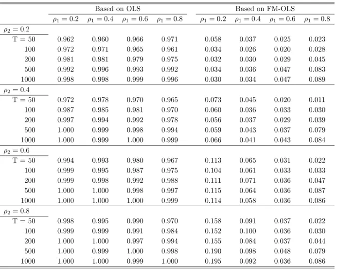
Table 4: Empirical Rejection Probabilities of the LM Test whenH0 is True

Based on OLS Based on FM-OLS

ρ1= 0.2 ρ1= 0.4 ρ1= 0.6 ρ1= 0.8 ρ1= 0.2 ρ1= 0.4 ρ1= 0.6 ρ1= 0.8 ρ2= 0.2 T = 50 0.962 0.960 0.966 0.971 0.058 0.037 0.025 0.023 100 0.972 0.971 0.965 0.961 0.034 0.026 0.020 0.028 200 0.981 0.981 0.979 0.975 0.032 0.030 0.029 0.045 500 0.992 0.996 0.993 0.992 0.034 0.036 0.047 0.083 1000 0.998 0.998 0.999 0.996 0.030 0.034 0.047 0.089 ρ2= 0.4 T = 50 0.972 0.978 0.970 0.965 0.073 0.045 0.020 0.011 100 0.987 0.985 0.981 0.970 0.060 0.036 0.033 0.030 200 0.997 0.994 0.992 0.978 0.056 0.037 0.029 0.039 500 1.000 0.999 0.998 0.994 0.059 0.043 0.037 0.079 1000 1.000 0.999 1.000 0.999 0.066 0.041 0.043 0.084 ρ2= 0.6 T = 50 0.994 0.993 0.980 0.967 0.113 0.065 0.031 0.022 100 0.999 0.995 0.987 0.975 0.104 0.061 0.033 0.033 200 0.999 0.998 0.992 0.988 0.111 0.071 0.036 0.047 500 1.000 1.000 0.998 0.997 0.115 0.064 0.036 0.087 1000 1.000 1.000 1.000 0.999 0.114 0.058 0.036 0.086 ρ2= 0.8 T = 50 0.998 0.995 0.990 0.970 0.158 0.091 0.037 0.022 100 0.999 0.999 0.991 0.984 0.152 0.100 0.036 0.030 200 1.000 1.000 0.997 0.994 0.155 0.084 0.037 0.044 500 1.000 0.999 1.000 0.998 0.190 0.098 0.048 0.079 1000 1.000 1.000 0.999 1.000 0.195 0.092 0.036 0.086

(33)

where we show kernel density estimates of the test statistics based on the 5,000 replications for the intermediate sample sizeT = 500. The kernel densities are based on using the Gaussian kernel with bandwidth chosen according to Silverman’s rule of thumb. The left graphs display the OLS based statistics and the right graphs display the FM-OLS based statistics. Noting the scales for the left graphs makes clear why the OLS based statistics lead to rejections of the null hypotheses almost throughout. The FM-OLS based tests’ densities in the right graphs remains remarkably unaffected by both serial correlation (upper panel) and endogeneity (lower panel).

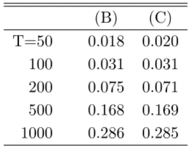
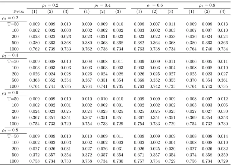
For studying the power performance of the LM test, i.e. the empirical rejection probabilities for DGPs different from the estimated equation, we consider three alternative DGPs given by

(A) : yt= 1 +t−15xt+ 5x2t −0.5x3t +ut

(B) : yt= 1 +t+ 5xt−0.3x2t +et, whereet is an I(1) variable independent ofxt

(C) : y_tand x_tare two independent I(1) variables To be precise in case (B) we use et =

P_t

j=1εt with εt ∼ N(0,4) and in case (C) yt is generated

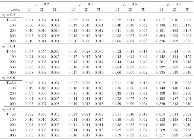
as y_t = Pt_j₌₁ε_t with ε_t ∼ N(0,1). The regressor x_t and for (A) u_t are throughout generated as described above. The three DGPs exemplify the main alternatives of interest. Alternative specifica-tion (A) covers the case of missing higher polynomial powers of the integrated regressor, alternative (B) corresponds to the case of a missing integrated regressor and alternative (C) corresponds to a spurious regression. The estimated equation is for all DGPs given by (18) and for alternative (A) again all combinations of ρ1 andρ2 are considered.

The results in case of alternative (A) are displayed in Table 5 and for alternatives (B) and (C) the results are shown in Table 6. The results in Table 5 show that power is close to 1 or equal to 1 in case of missing higher polynomial powers for already the smallest considered sample sizeT = 50. This finding is robust with respect to the amount of serial correlation and endogeneity. However, power is much lower in case of alternatives (B) and (C). Alternatives (B) and (C) are not as well captured by the regressors Ft as in case of alternative (A), in which case the inclusion ofFt leads

to a well-specified augmented regression. These results emphasize that the performance of the LM test depends, as in the stationary case, upon the relationship between the true but (in applications) unknown alternative and the auxiliary regressors collected in Ft. For empirical applications this

means that one might consider to perform the LM test with several sets of auxiliary regressors, ignoring as is usual in empirical work all problems related to performing multiple inference.

(34)

0 0.5 1 1.5 2 x 106 0 0.5 1 1.5 2 2.5 3 3.5 4 4.5 5x 10 −6 _{(1) Based on OLS} 0 5 10 15 0 0.05 0.1 0.15 0.2 0.25 0.3 0.35 0.4 0.45 0.5 (2) Based on FM Regression ρ 1=0.2 ρ 1=0.4 ρ 1=0.6 ρ 1=0.8

(a) Effect of Serial Correlation: T = 500,ρ2= 0.4

0 2 4 6 8 10 x 105 0 0.5 1 1.5 2 2.5 3 3.5 4 4.5 5x 10 −6 _{(1) Based on OLS} 0 5 10 15 0 0.05 0.1 0.15 0.2 0.25 0.3 0.35 0.4 0.45 0.5 (2) Based on FM Regression ρ 2=0.2 ρ 2=0.4 ρ 2=0.6 ρ 2=0.8 (b) Effect of Endogeneity: T = 500,ρ1= 0.4