DOI 10.1007/s10182-008-0053-6 O R I G I N A L PA P E R
A Markov chain Monte Carlo algorithm for multiple
imputation in large surveys
Daniel Schunk
Received: 15 September 2006 / Accepted: 19 March 2007 / Published online: 29 January 2008 © Springer-Verlag 2008
Abstract Important empirical information on household behavior and finances is obtained from surveys, and these data are used heavily by researchers, central banks, and for policy consulting. However, various interdependent factors that can be con-trolled only to a limited extent lead to unit and item nonresponse, and missing data on certain items is a frequent source of difficulties in statistical practice. More than ever, it is important to explore techniques for the imputation of large survey data. This paper presents the theoretical underpinnings of a Markov chain Monte Carlo multiple imputation procedure and outlines important technical aspects of the application of MCMC-type algorithms to large socio-economic data sets. In an illustrative applica-tion it is found that MCMC algorithms have good convergence properties even on large data sets with complex patterns of missingness, and that the use of a rich set of covariates in the imputation models has a substantial effect on the distributions of key financial variables.
1 Introduction
Important empirical information on household behavior and finances is obtained from surveys. However, various interdependent factors can be controlled only to a limited extent. Privacy concerns, respondent uncertainty, cognitive burden of the questions, and survey context, for example, can lead to unit nonresponse and item nonresponse. The general phenomenon of item nonresponse to questions in household surveys as well as problems of statistical analysis with missing data have been analyzed by various authors, beginning with the work by Ferber (1966) and Hartley and Hocking (1971); see Beatty and Herrmann (2002) as well as Rässler and Riphahn (2006) for reviews. Recent examples that focus on income, saving, and asset choice are Barceló
D. Schunk (
)Department of Empirical Research in Economics, University of Zurich, 8006 Zurich, Switzerland e-mail: [email protected]
(2006, Spanish Survey of Household Finances) and Kennickell (1998, U.S. Survey of Consumer Finances), as well as Biewen (2001), Frick and Grabka (2005), Riphahn and Serfling (2004), and Schräpler (2003) who worked with data from the German Socio-Economic Panel (GSOEP).
For a large majority of variables in household surveys, item nonresponse is not a problem. For example, in the context of the German SAVE survey—a survey that focuses on details of households’ finances as well as households’ socio-demographic and psychological characteristics—there is hardly any nonresponse to questions about socio-demographic conditions of the household, to questions about households’ expectations, health conditions, and about indicators of household economic behavior (Essig and Winter2003; Schunk2007). Mainly due to privacy concerns and cognitive burden, though, there are higher item nonresponse rates for detailed questions about a household’s financial circumstances. For studies that use this financial information, missing information on one of those variables is a problem. It is tempting and still very common to simply delete all observations with missing values. But deleting ob-servations with item nonresponse, i.e. relying on a complete-case analysis, might lead to an efficiency loss due to a smaller sample size and to biased inference when item nonresponse is related to the variable of interest.1Particularly for multivariate analy-ses that involve a large number of covariates, case deletion procedures can discard a high proportion of subjects, even if the per-item rate of missingness is rather low.
The purpose of this paper is to present and discuss the theoretical underpinnings of an iterative multiple imputation method that has been developed for large survey data. The paper also outlines key technical issues related to the application of MCMC-type algorithms to large data sets.2Missing item values are imputed controlling for observed characteristics of nonrespondents and respondents in order to preserve the correlation structure of the data set as much as possible. The method yields a multiply imputed and complete data set that can be analyzed without discarding any observed cases. In contrast to single imputation, multiple imputation allows the uncertainty due to imputation to be reflected in subsequent analyses of the data (see, e.g., Rubin1987, 1996; Rubin and Schenker1986).
Other iterative multiple imputation methods have recently been applied to large-scale socio-economic survey data. The imputation method for the U.S. Survey of Consumer Finances of the Federal Reserve Board System, developed by Arthur Ken-nickell and described in his seminal paper of this topic (KenKen-nickell1998), has been used on the Spanish Survey of Household Finances (Barceló 2006). However, the convergence properties of Markov chain Monte Carlo procedures have only been systematically analyzed on simulated data sets and on small data sets with only few variables (e.g., Schafer1997). Furthermore, there is only a limited discussion about the effects of imputation on the resulting distributions of imputed financial variables in the context of large-scale survey data. This discussion almost exclu-sively concerns noniterative approaches (Frick and Grabka2005; Hoynes et al.1998;
1See, e.g., Rubin (1987) and Little and Rubin (2002) for discussions about efficiency and bias in a missing
data context.
2A companion paper (Schunk2007) documents the application of this MCMC-method to the SAVE data in
detail, investigates the convergence properties, and analyzes the resulting distributions of various imputed variables.
Kalwij and van Soest2005). Discussing distributional effects, however, is informative for both survey and imputation methodology. First, it complements findings based on other imputation methods as well as based on experiments that investigate the mech-anisms of item nonresponse, and second, it is a contribution to the exploration of new imputation techniques for large surveys. Briefly, a discussion of the theoretical un-derpinnings of MCMC methods as well as of convergence issues and distributional effects serves to evaluate different imputation methods and is an important step in the scientific discussion about the development of standards for the imputation of large survey data.
2 An iterative multiple imputation method—motivation and theoretical underpinnings
To deal with item nonresponse, one can resort to a complete-case analysis, to model-based approaches that incorporate the structure of the missing data, or one can use imputation procedures.3A complete-case analysis may produce biased inference if the data set with only complete observations differs systematically from the target population; weighting of the complete cases reduces the bias but generally leads to inappropriate standard errors. Additionally, a complete-case analysis leads to less efficient estimates, since the number of individuals with complete data is often con-siderably smaller than the total sample size.4Formal modeling that incorporates the structure of the missing data involves basing inference on the likelihood or posterior distribution under a structural model for the missing-data mechanism and the incom-plete survey variables, where parameters are estimated by methods such as maximum likelihood. Multiple imputation is essentially a way to solve the modeling problem by simulating the distribution of the missing data (Rubin1996). Ideally, the imputation procedures control for all relevant differences between nonrespondents and respon-dents, such that the results obtained from the analysis of the complete data set are unbiased.
2.1 Assumptions
Many different statistical imputation methods exist and they are applied in a vari-ety of data contexts. Examples are mean or median imputation, hotdeck imputation, and regression-based imputation. Hotdeck is a very frequently used nonparametric method (e.g., in the RAND-HRS). For hotdeck, only very few conditioning variables can be used even when the data set is very large. Regression-based imputations need parametric assumptions. Since regression-based methods allow for conditioning on many more variables than hotdeck methods, they are better than hotdeck methods in preserving a rich correlation structure of the data, provided that an appropriate parametric assumption is made.
3An excellent overview of approaches to deal with item nonresponse was presented by Rässler and
Riphahn (2006).
4Rubin (1987) and Little and Rubin (2002) illustrated and discussed biased inference and efficiency losses
Ideally, in order to impute the missing values, a statistical model should be explic-itly formulated for each incomplete survey variable and for the missing-data mech-anism. The parameters should then be estimated from the existing data (and from potentially available further information, such as information about the interview process) by methods such as maximum likelihood. Identifying the probability dis-tributions of the variables under study is often very hard and requires very weakly motivated assumptions, since the mechanisms of nonresponse are often very com-plex (Manski2005).
Clearly, imputation methods have to make statistical assumptions about the non-response mechanism and about the distribution of the data values in the survey.5For the imputation method presented in this paper, the underlying assumption about the way in which missing data were lost is that missing values are ignorable.
The missing data mechanism is said to be ignorable if (a) the data are missing at random (MAR),6and (b) the parameters for the missing data-generating process are unrelated to the parameters that the researcher wants to estimate from the data.7 Ignorability is the formal assumption that allows one to estimate relationships among variables between observed data and then use these relationships to obtain predictions of the missing values from the observed values.
Of course, for these relationships to yield unbiased predictions, one would need the correct model for the observed and missing values. In practice, imputation meth-ods for large data sets rely on simple parametric assumptions or on nonparametric hotdeck methods for discrete variables with only a few categories and with very low rates of missingness.8
The fact that data have been imputed multiply increases robustness to departures from the true imputation model considerably compared to single imputation ap-proaches that are based on the same imputation model. This has been demonstrated in various simulation studies (Ezzati-Rice et al.1995; Graham and Schafer 1999; Schafer1997). Furthermore, existing research—using data sets from different scien-tific fields and with varying nonresponse rates—emphasizes the robustness of mul-tiple imputation to the specifically chosen imputation model, given that appropriate conditioning variables are available in the data set. These findings advocate the use of simple linear models (see, e.g., Schafer1997; Bernaards et al.2003).
5The Bayesian nature of the presented imputation algorithm also requires specification of a prior
distribu-tion for the parameters of the imputadistribu-tion model. In practice, unless the data are very sparse or the sample is very small, a noninformative prior is used (see Schafer1997for details). These conditions are rarely violated in data from serious socio-economic surveys. A noninformative prior can also be used for the SAVE data to which the presented MCMC algorithm has been applied (see Sect.3).
6See, e.g., Schafer (1997) for a definition of MAR and note that the MAR assumption cannot be tested
from available data (Cameron and Trivedi2005). Note also that MAR does not imply that the missing values are a random subsample of the complete data set. This latter condition is much more restrictive and is called “missing completely at random” (MCAR). See Little and Rubin (2002) and Cameron and Trivedi (2005) for further discussions.
7In the literature, MAR and ignorability are often treated as equivalent under the assumption that condition
(b) for ignorability is almost always satisfied.
8See, e.g., Barceló (2006), Frick and Grabka (2005), and Kennickell (1998). They generally assumed a
2.2 Multiple imputation
Single imputation does not reflect the true distributional relationship between ob-served and missing values and it does not allow uncertainty about the missing data to be reflected in the subsequent analyses. This leads to estimated standard errors that are generally too small. As documented and discussed by Li et al. (1991) and by Ru-bin and Schenker (1986), this can seriously affect the subsequent interpretation of the analyses.
In multiple imputation,M >1 plausible data sets are generated with all missing values replaced by imputed values. AllMcomplete data sets are then used separately for the analysis and the results of allManalyses are combined such that the uncer-tainty due to imputation is reflected in the results (see Rubin1987). Generally, this can involve two types of uncertainty: Sampling variation assuming the mechanisms of nonresponse are known and variation due to uncertainty about the mechanisms of nonresponse (Rubin1987).
Unless the fraction of missing data is extremely large, it is sufficient to obtain a relatively small number M of imputed data sets, usually not more than five. The relative gains in efficiency from larger numbers are minor under the rates of missing data that are observed in most socio-economic surveys.9
2.3 Stochastic imputation and conditioning variables
To preserve the correlation structure of the data, it is important to capture all rele-vant relationships between variables. In practice, the method therefore conditions on as many relevant and available variables as possible in the imputation of each sin-gle variable. All possible determinants of the variable to be imputed are included as predictors of that variable as well as their powers and interactions (e.g., Little and Raghunathan1997). Additionally, including all variables that are potential predictors of missingness makes the MAR assumption more plausible, because this assump-tion depends on the availability of variables that can explain missingness and that are correlated with the variable to be imputed (Schafer1997).
Each imputation model further imputes the missing data stochastically, such that the characteristics of the data distribution are preserved over the M imputed data sets. Suppose that the imputation model proposed for the variable of interest,y, is a simple linear model which is estimated based onnobservations andkconditioning variables:
y=Xβ+u, u|X∼N0, σ2I. (1) Stochastic imputation then replaces the missing valueyuby its best linear predicted
value,Xβ, plus a random drawu. This random draw comes from a normal distribu-tion:
yu=Xβ+u, u|X∼N
0,σ2I, (2)
9Rubin (1987) and Schafer (1997) defined efficiency in the context of multiply imputed data sets and
β=(XX)−1(Xy), σ2= 1 n−k
yy−yX(XX)−1Xy. (3) 2.4 Markov chain Monte Carlo simulation
Tanner and Wong (1987) presented an iterative simulation framework for imputa-tion based on an argument that involves the estimaimputa-tion of a set of parameters from conditioning information that is potentially unobserved. This section reviews their arguments and motivates an iterative imputation method that can be used for large surveys.
Letxu be unobserved values of a larger setx and letxo=x\xu.Xu is the
sam-ple space of the unobserved data,θ is a set of parameter values to be estimated for which the parameter space is denoted byΘ. The desired posterior distribution of the parameter values, given the observed data, can be written as
f (θ|xo)=
Xu
f (θ|xo, xu)f (xu|xo) dxu. (4)
Here,f (θ|xo, xu)is the conditional density ofθ given the complete data X, and
f (xu|xo)is the predictive density of the unobserved data given the observed data.
The predictive density of the unobserved data given the observed data can be related to the posterior distribution that is shown above as
f (xu|xo)=
Θ
f (xu|φ, xo)f (φ|xo) dφ. (5)
Tanner and Wong’s (1987) basic idea is that the desired posterior is intractable based on only the observed data, but it is tractable after the data are augmented by unobserved data xu in an iterative framework. The suggested iterative method for
the calculation of the posterior starts with an initial approximation of the posterior. Then, a new draw of xu is made from f (xu|xo)given the current draw from the
posteriorf (θ|xo), and this draw is then used for the next draw off (θ|xo). Tanner
and Wong showed that under mild regularity conditions, this iterative procedure con-verges to the desired posterior.
In an imputation framework, the target distribution is the joint conditional distri-bution ofxu andθ, givenxo. Based on the ideas of Tanner and Wong, the iterative
simulation method is summarized as follows: First, replace all missing data by plau-sible starting values. Given certain parametric assumptions,θ can then be estimated from the resulting complete data posterior distributionf (θ|xo, xu). Now letθt be the
current value ofθ. The next iterative sample ofxu can then be drawn from the
pre-dictive distribution ofxugivenxoandθt:
xut+1∼fxu|xo, θt
[Imputation step (I-step)]. (6) The next step is again to simulate the next iteration of θ from the complete data posterior distribution:
θt+1∼fθ|xo, xut+1
Repeating steps (6) and (7), i.e. sequential sampling from the two distributions, gener-ates an iterative Markovian procedure{(θt, xtu):t=1,2, . . . , N}. For the purpose of imputation, this procedure yields a successive simulation of the distribution of miss-ing values, conditioned on both observed data and distributions of missmiss-ing data previ-ously simulated. The set of conditioning variables in this algorithm is not necessarily the entire set of all possible values (Tanner and Wong 1987). Geman and Geman (1984) applied a similar procedure in the field of image processing and showed that the stochastic sequence is a Markov chain that has the correct stationary distribution under certain regularity conditions. Li (1988) presented an additional formal argu-ment that, with each iteration, the process moves closer to the true latent distribution and finally converges. The method is called Markov chain Monte Carlo (MCMC) because it involves simulation and the sequence is a Markov chain. Formally, the method is also related to Gibbs sampling (Hastings1970), and in the missing data literature it is often referred to as data augmentation. This method has been used in many statistical applications (e.g., Barceló2006; van Buuren et al.1999; Kennickell 1998; Schafer1997; Schunk2007). Sequential simulation algorithms of the MCMC-type can be modified and implemented in different ways; I briefly come back to this issue in Sect.4.
3 The iterative multiple imputation method for SAVE
The iterative multiple imputation method described in the previous section was ap-plied to the German SAVE data. This section outlines the algorithmic structure of this implementation in order to draft the central features of an application of a Markov chain Monte Carlo-type algorithm to a large data set with complex patterns of miss-ingness. Furthermore, it summarizes briefly the main results of this application.10 3.1 Algorithmic overview
The multiple imputation method for SAVE (MIMS) distinguishes between core vari-ables and noncore varivari-ables. The core varivari-ables have been chosen such that they cover the financial modules of the survey that involve all questions related to income, sav-ings, and wealth of the household. The noncore variables include socio-demographic, psychometric, and health variables, as well as indicator variables for household eco-nomic behavior. All core variables have missing rates of at least 4%. The noncore variables have considerably lower missing rates, in almost all cases much less than 2%. The following 136 variables (grouped into three categories) are defined as core variables:
• Income variables (E): 41 binary, ordinal, and continuous variables.
• Savings variables (S): 3 binary and continuous variables.
• Asset and Credit variables (A): 92 binary and continuous variables.
10A detailed documentation and discussion of this application is provided in a companion paper (Schunk 2007).
All other variables in the data set are noncore variables.
To facilitate the algorithmic description, all variables are categorized as follows: • All variables that are not core variables are called other variables, O.
• P is a subset of O, the subset of all variables that are used as conditioning variables or predictors for the current imputation step.
• The union of all variables from P and all core variables that are used as con-ditioning variables for the current imputation step is referred to as the set C (=conditioning variables). In the following algorithmic description, C always contains the updated information based on the most recent iteration step, and it contains the maximum number of variables on which one can condition.
The complete imputation algorithm for the SAVE data works as follows: – Impute all variables using logical imputation whenever possible. Outer Loop – REPEAT 5 times,j=1, . . . ,5(=generate 5 data sets)
– Impute variables from O using (sequential) hotdeck imputation, obtain complete data O∗.
– Impute the income variablesEusing P∗, obtain complete data E∗. – Impute the savings variablesSusing P∗and E∗, obtain complete data S∗. – Impute the asset variablesAusing P∗, E∗, and S∗, obtain complete data A∗. Inner Loop – REPEATN times(=iterateN times)
– Impute the income variablesEusing C. – Impute the savings variablesSusing C. – Impute the asset variablesAusing C. Inner Loop – END
Outer Loop – END
MIMS follows a fixed path through the data set, and the five repetitions in the outer loop each generate one imputed data set. Thus, five complete data sets are obtained. The first step of the procedure consists of logical imputation. In many cases, the complex tree structure of the SAVE survey or cross-variable relationships allow for the possibility to logically impute missing values. The following path through the data set is guided by the knowledge of the missing item rates and by cross-variable relationships. The path starts with variables with low missing rates, such that those variables can subsequently be used as conditioning variables for other variables with higher missing rates. For example, among the core variables, the net income variable is imputed first, since its missing rate is generally lower than the missing rates of other core variables. The algorithmic description shows that as soon as the iteration loop starts, all variables are already imputed, i.e. starting values for the iteration process have been obtained, and all variables can be used as conditioning variables during the iteration.11Each variable is imputed based on one of the following three general methods:12
11One referee has argued that the algorithm should condition on further core variables for choosing starting
values. It is found that the choice of different starting values neither changes the findings on convergence nor the findings about the resulting distributions of the imputed variables (see Schunk2007).
12These methods and their application to binary, categorical, ordinal and (quasi-)continuous variables with
(1) For all categorical or ordinal variables with only few categories and with a low missing rate, a hotdeck procedure with several conditioning variables is used. (2) For all binary, categorical, or ordinal core variables, binomial or ordered probit
models are used.
(3) For all continuous or quasi-continuous variables, randomized linear regressions with normally distributed errors are used. The conditional expected value is es-timated and an error term, drawn from a symmetrically censored normal distri-bution, is added. This normal distribution has mean zero and its variance is the residual variance of the estimation. The error term is always restricted to the central three standard deviations of the distribution in order to avoid imputing extreme values. In a few cases, logical or other constraints require that the error term be further restricted; examples are non-negativity constraints. The imputed value is also restricted to lie in the observed range of values for the corresponding variable. That is, in particular, imputed values will not be higher than observed values for a certain variable.
Due to the skip patterns in the questionnaire, the data have a very complex tree structure that imposes a logical structure which has to be accounted for in the im-putation process. Furthermore, the imputed values have to satisfy potential logical conditions imposed by the information provided by the households or imputed previ-ously. If necessary, the procedure draws from the estimated conditional distribution until an outcome is found that satisfies all possible constraints that apply in the par-ticular case.
3.2 Selection of conditioning variables
As is clear from the description above, each regression or hotdeck method is tailored specifically to the variable to be imputed. Of particular importance are the condition-ing variables which have been selected individually for every scondition-ingle variable with missing information according to the following guidelines:
(A) Hotdeck imputations: Hotdeck imputations, which are used for discrete variables with very low missing rates, allow for only few and discrete conditioning variables due to the quickly increasing number of corresponding conditioning cells. The condi-tioning variables are first selected based on theoretical relationships if available and, second, based on the strength of the respective correlation with the variable to be imputed.
(B) Regression-based imputations: In theory, every regression-based imputation should use all relevant variables in the data set, as well as higher powers and in-teractions of those terms as conditioning variables (Little and Raghunathan 1997). The imputation procedure should, in particular, attempt to preserve the relationships between all variables that might be jointly analyzed in future studies based on the imputed data (Schafer1997). In practice, a limit to the number of included condition-ing variables is imposed by the degrees of freedom of the regressions. Additionally, there must not be collinearity between conditioning variables, which can easily arise in some cases due to the tree structure of the questions. Due to these constraints concerning the inclusion of conditioning variables, it is of particular importance to
select these variables following a procedure that ensures the best possible use of the available information (see Schunk2007).
3.3 Results
MIMS has been applied to the 2003/2004 wave of the SAVE survey which contains 3,154 observed households. This section outlines the key issues and findings concern-ing the assessment of convergence as well as concernconcern-ing the effect of the algorithm on the distribution of the imputed data.
3.3.1 Convergence of MIMS
Assessing convergence of the sequence of draws to the target distribution is more difficult than assessing convergence of, e.g., EM-type algorithms, because there is no single target quantity to monitor, like the maximum value of the likelihood. Two convergence criteria have been used: First, a criterion that is based on a measure for the average change in the values of a certain variable vector between two consecutive iteration steps (see Schunk2007). Second, a standard convergence criterion that was also mentioned by Barceló (2006) and which is defined with respect to measures of position and dispersion of the distribution of the imputed variable:
b(t )= Q50Y t (Q75−Q25)Y t − Q50Y t−1 (Q75−Q25)Y t−1 Q50Y t (Q75−Q25)Y t − Q50Y t−1 (Q75−Q25)Y t−1 . (8)
Here, Q25, Q50, and Q75 denote the 25th, 50th, and 75th quantile, respectively, of the particular distribution of imputed values.
Based on both criteria, the convergence analysis finds quick convergence of the algorithm on all variables. Although some variables have already converged after one iteration step, others need about ten iteration steps. No indication of divergent behav-ior or long-term drift was found even after running the algorithm for 1,000 iteration steps. Given these findings about convergence, MIMS is run for 20 iteration steps, i.e. N =20. This is in line with findings based on the iterative algorithm implemented for the Survey of Consumer Finances (Kennickell1998). Kennickell reports quick convergence on key variables, the SCF algorithm is run for six iteration steps.
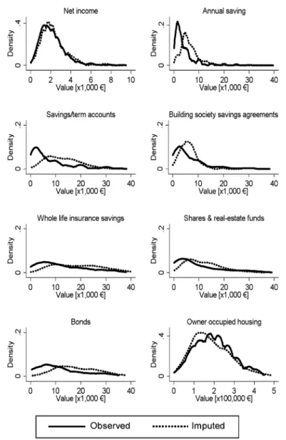
3.3.2 Imputed and observed data
Figure1 shows the estimated distributions of imputed and observed values for six selected variables.13 It is evident that the inclusion of covariates has a substantial effect on the distribution of asset holdings, a conclusion emphasized by various au-thors who used other methods (Chand and Gan2002; Kalwij and van Soest2005; Hoynes et al.1998). For most financial asset items, the included conditioning vari-ables shift the distribution to higher values on average, compared to the original dis-tribution of observed values, which would simply be replicated if no conditioning
13The kernel density is estimated for positive values of the variables that have been analyzed above; an
Epanechnikov kernel and Silverman’s rule of thumb (Silverman1986) for bandwidth selection have been used.
Fig. 1 Density functions of observed and imputed values
variables were used. In contrast to the findings concerning the financial wealth vari-ables, imputed variables of owner occupied housing are lower than observed values. The findings on the effect on financial wealth as well as on owner occupied housing wealth are in line with, e.g., Hoynes et al. (1998) who used a noniterative regression-based imputation. Concerning the income values, a detailed analysis also reveals that MIMS does not have a strong effect on their distribution. Item nonresponse seems to be only mildly selective with respect to the tails of the income distribution, and mean imputed income is slightly higher than mean observed income. The nature of both effects corresponds to the effects reported by Frick and Grabka (2005). Their
find-ings from a regression-based single-imputation procedure of annual income variables for the SOEP suggest that item nonresponse on income appears to be selective with respect to both tails of the income distribution; the overall effect of their imputation is an increase in the mean of after-tax income by 1.7%.
4 Discussion and conclusion
Except for controlled experimental settings, survey-based studies about human past and intended behavior rarely generate complete information. For several reasons, dis-cussed in this paper, it is nevertheless desirable to provide users with a complete data set in which all missing values have been imputed.
The goal of this paper is to present the theoretical underpinnings of a Markov chain Monte Carlo imputation method as well as to outline technical issues related to the application of MCMC-type algorithms to large data sets with complex patterns of missingness. Since missing values are rarely known with certainty, the presented algorithm generates multiply imputed data. This ensures that the uncertainty about the missing data can be appropriately reflected in subsequent analyses.
The Markov chain Monte Carlo technique that is used for the algorithm developed in this paper is similar to the method presented by Schafer (1997), who used smaller data sets with only few conditioning variables and to the method used in Kennickell (1998). Based on the presented theoretical deliberations, it is clear that modifications of this implementation—which might have different convergence properties in prac-tice but should have the same stationary distribution—are conceivable. For example, in each iteration step, the distribution of unobserved values can be simulated a certain number of timesp, and the parameter values for the next iteration step can then be estimated from allpsimulated distributions; this means that multiple versions of the unobserved data are generated from the predictive distribution in one iteration step. This modification has also been implemented for the SAVE data and the findings are perfectly in line with the results presented in this paper, both in terms of distri-butional effects as well as in terms of convergence properties. Other modifications are conceivable and should be explored in the future. The sequential simulation al-gorithm can be modified such that each draw from a certain conditional distribution depends not only on the conditional distribution estimated in the preceding iteration step, but also on conditional distributions estimated in earlier iteration steps. A com-parison of convergence properties between different ways of implementing the data augmentation algorithm would be helpful.
So far, convergence properties of MCMC methods have only been systematically analyzed on simulated data sets and data sets with fewer variables compared to the large household survey that is analyzed in this paper. The findings of the present il-lustrative study suggest that the algorithm converges in only few iteration steps on large data sets with complex patterns of missingness. For most variables, the process is stationary after not more than about 5–10 iteration steps. For all other variables, it is stationary from the first iteration step on, suggesting that the algorithm has al-ready converged in the first iteration step. It is certainly worthwhile to investigate the convergence properties of MCMC algorithms in the context of large surveys or large
simulated data sets in a collaborative effort and with standardized methods. This will further contribute to a more comprehensive evaluation of the relevance of MCMC methods for survey research.
Finally, a comparison between imputed and observed values has revealed that the use of covariates in the imputation process has a substantial effect on the distribu-tions of individual asset holdings. In general, these effects are similar to the effects reported based on other techniques. This finding suggests that item nonresponse is not occurring randomly but is related to the included covariates. The analyses also sug-gest that there might be differences in the character of nonresponse across asset types, and they indicate specific directions for future research on the relationship between socio-economic characteristics and nonresponse to specific items. Furthermore, from the point of view of survey methodology and data quality management—which is of ultimate interest for every researcher and policy maker—the findings underline the need for an ongoing scientific discussion about imputation. In particular, this discussion will have to do with the effects of different imputation strategies on the distribution of data obtained in large-scale socio-economic surveys as well as with a systematic exploration of the feasibility of different imputation methods.
Acknowledgements I gratefully acknowledge many astute comments by Axel Börsch-Supan, Joachim Frick, Michael Hurd, Arthur Kennickell, Enno Mammen, Susanne Rässler, Arthur van Soest, Guglielmo Weber, and Joachim Winter, as well as seminar participants at the University of Mannheim and the con-ference on statistical imputation methods in Bronnbach. I am particularly indebted to Arthur Kennick-ell for his invaluable advice. Gunhild Berg, Armin Rick, Frank Schilbach, Bjarne Steffen and Michael Ziegelmeyer provided excellent research assistance. Financial support was provided by the Deutsche Forschungsgemeinschaft (via Sonderforschungsbereich 504 at the University of Mannheim).
References
Barceló, C.: Imputation of the 2002 wave of the Spanish Survey of Household Finances (EFF). Occasional Paper No. 0603, Bank of Spain (2006)
Beatty, P., Herrmann, D.: To answer or not to answer: Decision processes related to survey item nonre-sponse. In: Groves, R.M., Dillman, D.A., Eltinge, J.L., Little, R.J.A. (eds.) Survey Nonresponse, pp. 71–85. Wiley, New York (2002)
Bernaards, C.A., Farmer, M.M., Qi, K., Dulai, G.S., Ganz, P.A., Kahn, K.L.: Comparison of two multiple imputation procedures in a cancer screening survey. J. Data Sci. 1(3), 293–312 (2003)
Biewen, M.: Item non-response and inequality measurement: Evidence from the German earnings distrib-ution. Allg. Stat. Arch. 85(4), 409–425 (2001)
Cameron, A.C., Trivedi, P.K.: Microeconometrics. Methods and Applications. Cambridge University Press, New York (2005)
Chand, H., Gan, L.: Wealth item nonresponse and imputation in the AHEAD. Working Paper, Texas A&M University (2002)
Essig, L., Winter, J.: Item nonresponse to financial questions in household surveys: An experimental study of interviewer and mode effects. MEA-Discussion paper 39-03, MEA—Manheim Research Institute for the Economics of Aging, University of Mannheim (2003)
Ezzati-Rice, T.M., Johnson, W., Khare, M., Little, R.J.A., Rubin, D.B., Schafer, J.L.: Multiple imputation of missing data in NHANES III. In: Proceedings of the Annual Research Conference, pp. 459–487, U.S. Bureau of the Census (1995)
Ferber, R.: Item nonresponse in a consumer survey. Public Opin. Q. 30(3), 399–415 (1966)
Frick, J.R., Grabka, M.M.: Item nonresponse on income questions in panel surveys: Incidence, imputation and the impact on inequality and mobility. Allg. Stat. Arch. 90(1), 49–62 (2005)
Geman, S., Geman, D.: Stochastic relaxation, Gibbs distribution, and the Bayesian restoration of images. IEEE Trans. Pattern Anal. Mach. Intell. PAMI-6(6), 721–741 (1984)
Graham, J.W., Schafer, J.L.: On the performance of multiple imputation for multivariate data with small sample size. In: Hoyle, R. (ed.) Statistical Strategies for Small Sample Research, pp. 1–29. Sage, Thousand Oaks (1999)
Hartley, H.O., Hocking, R.R.: The analysis of incomplete data. Biometrics 27, 783–808 (1971)
Hastings, W.K.: Monte Carlo sampling methods using Markov chain and their applications. Biometrika 57, 97–109 (1970)
Hoynes, H., Hurd, M., Chand, H.: Household wealth of the Elderly under alternative imputation proce-dures. In: Wise, D.A. (ed.) Inquiries in the Economics of Aging, pp. 229–257. The University of Chicago Press, Chicago (1998)
Kalwij, A., van Soest, A.: Item non-response and alternative imputation procedures. In: Börsch-Supan, A., Jürges, H. (eds.) The Survey of Health, Ageing and Retirement in Europe—Methodology, pp. 128–150. Mannheim Research Institute for the Economics of Aging, Mannheim (2005)
Kennickell, A.B.: Multiple imputation in the survey of consumer finances. In: Proceedings of the 1998 Joint Statistical Meetings, Dallas, TX (1998)
Li, K.: Imputation using Markov chains. J. Stat. Comput. Simul. 30, 57–79 (1988)
Li, K., Raghunathan, T., Rubin, D.: Large sample significance levels from multiply-imputed data using moment-based statistics and anFreference distribution. J. Am. Stat. Assoc. 86, 1065–1073 (1991) Little, R.J.A., Rubin, D.B.: Statistical Analysis with Missing Data. Wiley, New York (2002)
Little, R.J.A., Raghunathan, T.: Should imputation of missing data condition on all observed variables? In: Proceedings of the Section on Survey Research Methods, Joint Statistical Meetings, Anaheim, California (1997)
Manski, C.: Partial identification with missing data: Concepts and findings. Int. J. Approx. Reason. 39(2– 3), 151–165 (2005)
Rässler, S., Riphahn, R.: Survey item nonresponse and its treatment. Allg. Stat. Arch. 90, 217–232 (2006) Riphahn, R., Serfling, O.: Item non-response on income and wealth questions. Empir. Econ. 30(2), 521–
538 (2004)
Rubin, D.B.: Multiple Imputation for Nonresponse in Surveys. Wiley, New York (1987) Rubin, D.B.: Multiple imputation after 18+ years. J. Am. Stat. Assoc. 91(434), 473–489 (1996) Rubin, D.B., Schenker, N.: Multiple imputation for interval estimation from simple random samples with
ignorable nonresponse. J. Am. Stat. Assoc. 81(394), 366–374 (1986)
Schafer, J.L.: Analysis of Incomplete Multivariate Data. Chapman & Hall, London (1997)
Schunk, D.: A Markov chain Monte Carlo multiple imputation procedure for dealing with item nonre-sponse in the German save survey. MEA-Technical Discussion Paper 121-07, MEA—Manheim Re-search Institute for the Economics of Aging, University of Mannheim (2007)
Schräpler, J.-P.: Gross income non-response in the German socio-economic panel: Refusal or don’t know? Schmollers Jahrb. 123, 109–124 (2003)
Silverman, B.W.: Density Estimation for Statistics and Data Analysis. Chapman and Hall, London (1986) Tanner, M.A., Wong, W.H.: The calculation of posterior distributions by data augmentation. J. Am. Stat.
Assoc. 82(398), 528–550 (1987)
van Buuren, S., Boshuizen, H.C., Knook, D.L.: Multiple imputation of missing blood pressure covariates in survival analysis. Stat. Med. 18, 681–694 (1999)