A Bayesian Model for Brain Network Functional Connectivity using PyMC3

(1)

A Bayesian Model for Brain Network

Functional Connectivity using PyMC3

By Rui Wang

Thesis

Submitted to the Faculty of the Graduate School of Vanderbilt University

in partial fulfillment of the requirements for the degree of

MASTER OF SCIENCE in Biostatistics August 10, 2018 Nashville, Tennessee Approved: Hakmook Kang, Ph.D. Qingxia Chen, Ph.D.

(2)

ii

(3)

iii

ACKNOWLEDGEMENTS

First, I would like to express my sincere gratitude to my M.S. thesis advisor, Dr. Hakmook Kang. Without his comprehensive knowledge in the fields of biostatistics and brain imaging, it would be impossible for me to complete this interdisciplinary project involving biostatistical modeling and neuroscience imaging. In addition, I greatly thank Dr. Warren Taylor for offering the financial support and research opportunities and Dr. Christopher Fonnesbeck for his guidance of applying PyMC3 into my research. Furthermore, it is my great honor to work together with the committee member, Dr. Qingxia Chen for taking time to review this thesis and offer suggestions.

I am also grateful for the Department of Biostatistics when it enrolled me into this awesome program in 2016. Particularly, I would like to thank Dr. Jeffrey Blume for his dedicated instructions during the recent two years. I also appreciate all the faculty members in the department for their high-quality teaching, which motivates me to gain more knowledge beyond the experimental sciences. Besides, I would like to thank outstanding students, Sandya Lakkur, David Schlueter and Ya-Chen Lisa Lin for sharing their own experience of implementing related models and tools.

Finally, I would like to thank my family and friends. My mom and dad were able to provide the financial support in the recent two semesters. Minchun Zhou motivated me to complete 2017 Philadelphia full marathon. Dr. Changlin Zhang, Dr. Jun Liu, Dr. Xin Kou and Dr. Guo Li, friends of mine at college and Kaggle community, provided me with insights and encouragements when seeking career directions and industry employment.

(4)

iv

LIST OF TABLES

Page Table 2.1 Various common covariance functions from Ref [35]. ... 10 Table 2.2 Median (standard deviation), credible intervals (2.5% and 97.5% quantiles) of estimated functional connectivity, the Gelman Rubin diagnostic and the effect sample size under the condition of true structural connectivity and structural independence. ... 20 Table 2.3 Descriptive statistics of 41 subjects including control (n=23) and MDD (n=18) groups. ... 25 Table 2.4 Variable selection results from each method. ... 29

(6)

vi

LIST OF FIGURES

Page Figure 1.1 Venn diagram showing the studies combining functional and anatomical data, with focus on anatomical and functional connectivity data. Image reprinted with permission from Ref [4]. Copyright © 2007, John Wiley and Sons. ... 2 Figure 1.2 Resting-state fMRI studies capture the correlation between spontaneous activation patterns of brain regions. (a) The blood oxygen level-dependent (BOLD) signal is measured throughout the experiment. (b) Conventional task-dependent fMRI can be used to select a seed region of interest. (c) To examine the level of functional connectivity, the resting-state time-series of the seed voxel 𝑖 is correlated with the resting-state time-series of region 𝑗. (d) Furthermore, to map out all functional connections of the selected seed region, the time-series of the seed voxel 𝑖 can be correlated with the time-series of all other voxels in the brain, resulting in a functional connectivity map that reflects the regions that show a high level of functional connectivity with the selected seed region. Image reprinted with permission from Ref [1]. Copyright © 2010, Elsevier Inc. ... 3 Figure 1.3 Schematic of the basic principles underlying DTI: isotropy and anisotropy of water motion in tissue. The ellipsoids represent the directionality and the degree of anisotropy. The axes in these ellipsoids are oriented along the diffusion tensor eigenvectors, and the lengths of these axes are proportional to the amount of diffusivity (corresponding eigenvalues) in the respective dimensions. Image reprinted with permission from Ref [4]. Copyright © 2007, John Wiley and Sons. ... 5 Figure 2.1 Schematic of a direct structural connection between 𝑖 and 𝑗 ROIs and a possible indirect structural connection via 𝑘 ROI. ... 12 Figure 2.2 Histogram plots of 10 parameters from their posterior distribution. ... 22 Figure 2.3 Histogram plots of 10 parameters with 1000, 2000 and 3000 sample draws. .... 23 Figure 2.4 Correlation plot of covariates and estimated functional connectivity. ... 26

(7)

vii

ABSTRACT

Our brain network, as a complex integrative system, consists of many different regions. Each region has its own task and function and simultaneously shares structural and functional information. With the developed imaging techniques such as functional magnetic resonance imaging (fMRI) and diffusion tensor imaging (DTI), researchers can investigate the underlying brain functions related to human behaviors and some diseases or disorders in the nervous system such as major depressive disorder (MDD).

In this thesis, we developed a Bayesian hierarchical spatiotemporal model that combined fMRI and DTI data jointly to enhance the estimation of resting-state functional connectivity. Structural connectivity from DTI data was utilized to construct an informative prior for functional connectivity based on resting-state fMRI data through the Cholesky decomposition in a mixture model. The analysis took the advantages of probabilistic programming package as PyMC3 and next-generation Markov Chain Monte Carlo (MCMC) sampling algorithm as No-U-Turn Sampler (NUTS). The simulation study with this advanced algorithm, illustrated reduced mean squared errors (MSEs) of estimation. Furthermore, through a case study of MDD, we applied our model to examine how the estimated functional connectivity was associated with tasks of episodic memory, executive function, processing speed and working memory.

(8)

1

INTRODUCTION TO BRAIN CONNECTIVITY

1.1 Brain Imaging

Our brain consists of many different regions that have each own task and function [1]. As a complex integrative system, the brain network is formed when information is simultaneously processed and transported between structurally and functionally linked brain regions. The studies of brain network apply various techniques to either directly or indirectly image the structure and function of the nervous system. It is highly associated with the fields of medicine, neuroscience and psychology. Currently there are two main categories: one is structural imaging, involving with the structure of the nervous system and the diagnosis of intracranial diseases and disorders on a larger scale; the other is functional imaging, related with the diagnosis of metabolic diseases on a finer scale such as Alzheimer’s disease. It is fundamental for humans to understand how a healthy nervous system can produce activities such as thought, emotion and physical behavior, and regulate body functions to investigate some diseases and disorders.

In the recent decades, magnetic resonance imaging (MRI), a highly versatile imaging technique, was created by Peter Mansfield and Paul Lauterbur to capture the pictures of anatomy and the physiological process of the body in both health and disease. Due to their advanced breakthrough, they were awarded the 2003 Nobel Prize in Physiology or Medicine for their “discoveries concerning magnetic resonance imaging”. In the 1990s, functional magnetic resonance imaging (fMRI) was developed and it has been leading the brain mapping field because of its low invasiveness, lack of radiation exposure, relatively wide availability [2].

(9)

2

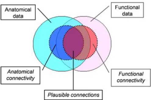
With all the developed imaging techniques, the studies of brain are focused on the structural and functional connectivity between two or more brain regions. Structural connectivity (also called anatomical connectivity) is referred as a structural link or the existence of neural connections between two regions while functional connectivity is defined as the temporal correlation between spatially remote neurophysiological events [3]. In other words, two systems can be assumed to be functionally connected if they illustrate synchronized or correlated patterns of activity [4]. The relationship between structural and functional connectivity is illustrated in Figure 1.1 in the form of a Venn diagram [4]. It highlights that the structural information could offer plausible arguments for the functional information.

Figure 1.1 Venn diagram showing the studies combining functional and anatomical data, with focus on anatomical and functional connectivity data. Image reprinted with permission from Ref [4]. Copyright © 2007, John Wiley and Sons.

(10)

3 1.2 Functional Connectivity

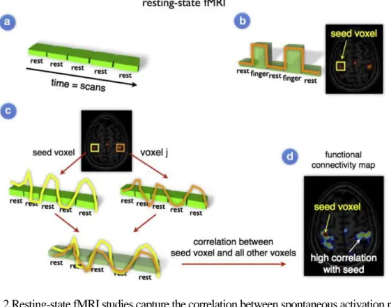
Figure 1.2 Resting-state fMRI studies capture the correlation between spontaneous activation patterns of brain regions. (a) The blood oxygen level-dependent (BOLD) signal is measured throughout the experiment. (b) Conventional task-dependent fMRI can be used to select a seed region of interest. (c) To examine the level of functional connectivity, the resting-state time-series of the seed voxel 𝑖 is correlated with the resting-state time-series of region 𝑗. (d) Furthermore, to map out all functional connections of the selected seed region, the time-series of the seed voxel 𝑖 can be correlated with the time-series of all other voxels in the brain, resulting in a functional connectivity map that reflects the regions that show a high level of functional connectivity with the selected seed region. Image reprinted with permission from Ref [1]. Copyright © 2010, Elsevier Inc.

Functional connectivity is typically measured by analyzing the patterns of concurrent activity between various brain areas that share functional properties. It is also defined as the

(11)

4

temporal dependency between spatially remote neurophysiological events [5, 6]. With deep understanding of fMRI in the recent two decades, more and more studies imply functional connectivity between brain areas as the level of co-activation of spontaneous fMRI time-series recorded at rest [7-9]. In the resting-state experiments, their level of spontaneous brain activity was recorded when subjects were required to relax without thinking anything. Typically, they are placed into the scanner, asked to close their eyes and to think nothing without falling asleep. Experimental evidences demonstrate that the left and right hemispheric regions of the primary motor network at rest show a high correlation between their fMRI time-series [9, 10], indicating the ongoing information transporting and ongoing functional connectivity between these areas at rest [7, 8, 10, 11]. Figure 1.2 illustrates that the state timeseries of a voxel in the motor network was correlated with the resting-state time-series of all other brain voxels, suggesting a high correlation between the spontaneous neuronal activation patterns of these areas. Therefore, resting-state fMRI research focuses on mapping functional communication channels between different brain regions by leveraging the correlated dynamics of fMRI time-series.

1.3 Structural Connectivity

Structural connectivity is typically pointed as the illustration of fiber tracts directly connecting different brain regions. Because of the neuronal axons in these fiber tracts, they can transmit the neural signals across all the brain areas, allowing for communications between brain regions. Previously, it has been applied to study animal with histological methods while it could not reveal much information in humans. Thanks to the advanced development of in vivo imaging techniques, researchers are now able to visualize the white matter. The volumetric estimates of while matter can be used as measures of structural

(12)

5

connectivity [12]. For example, it was found that the degree of while matter preservation in the groups of older adults is highly associated with their performance on tasks that require functional integration involving interhemispheric interactions [4].

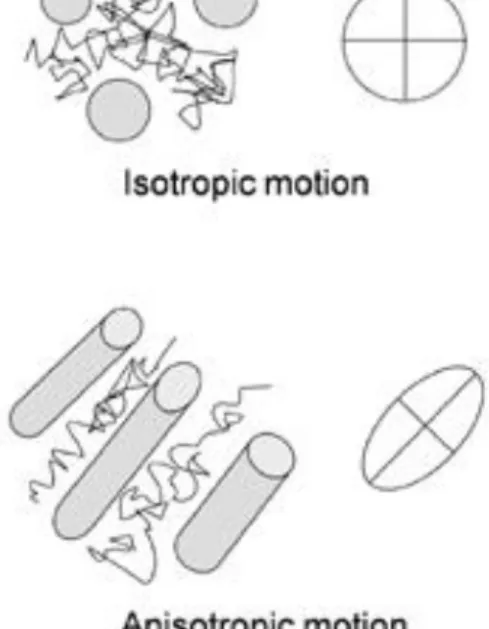
Figure 1.3 Schematic of the basic principles underlying DTI: isotropy and anisotropy of water motion in tissue. The ellipsoids represent the directionality and the degree of anisotropy. The axes in these ellipsoids are oriented along the diffusion tensor eigenvectors, and the lengths of these axes are proportional to the amount of diffusivity (corresponding eigenvalues) in the respective dimensions. Image reprinted with permission from Ref [4]. Copyright © 2007, John Wiley and Sons.

In the recent few years, a new imaging technology, diffusion tensor imaging (DTI) has been developed as a promising method for describing the structural connectivity in vivo. DTI is significant when the neural axons of while matter in the brain has an internal fibrous structure. Water will then diffuse more rapidly in the direction aligned with the internal structure while it moves more slowly in the perpendicular direction. So, DTI yields images

(13)

6

of the anisotropy of water diffusion in the living tissue. Figure 1.3 demonstrates the isotropy and anisotropy of water motion in tissue. Due to the increasingly accurate estimation of fiber orientation/strength and the widespread potential implications, DTI technology will shed light on the development of brain research in the future.

(14)

7

SPATIOTEMPORAL HIERARCHICAL MODEL

2.1 Existing Methods

As introduced in CHAPTER 1, functional connectivity is used as a biomarker for neurological and psychiatric disorders such as Alzheimer’s diseases [13, 14] and bipolar disorders [15, 16]. White matter tracts are the structural pathways of our brain, allowing the information to transmit between various brain areas. With the assistance of DIT data to reconstruct the white matter pathways, it demonstrates the links between structural connectivity and resting-state functional networks [17]. Many existing statistical methods have been developed to analyze fMRI data [18-21] and DTI data [22-25] within a Bayesian framework, separately. For example, a spatial and temporal independent component analysis (ICA) together with Bayesian approximation was applied to process large scale resting-state fMRI data from 200 subjects [21]. A multi-tensor Bayesian model with a new parameterization method was developed for DTI data from a healthy subject, allowing to be suitable for model selection in the post analysis via thresholding the Bayes factor [25].

Some efforts have been made to develop statistical models to combine fMRI data and DTI data jointly. A combined analysis of DTI and fMRI data was conducted to explore whether there were networks of regions where maturation of white matter and changes in brain activity showed similar developmental trends during childhood [26]. In this fMRI data analysis, functional anisotropy, as an indicator of myelination and axon thickness, was used as a covariate in a multiple regression model to find brain regions where functional anisotropy values and blood oxygen level-dependent (BOLD) response were correlated [26].

(15)

8

Another statistical method implementing a hierarchical clustering algorithm, combined various sources of data including anatomically weighted functional connectivity (awFC), fMRI and DTI data, to determine the functional connectivity [27]. What’s more, DTI data was utilized as a supplement of fMRI information, to estimate functional connectivity in a multimodal approach. This Bayesian model can determine the hierarchy among functional connected pairs of brain regions based on the associated probabilities of elevated activity for each node [28]. Other studies also demonstrated the superior advantages of using both fMRI and DTI data to investigate the functional connectivity in brain networks [29-33].

2.2 Spatiotemporal Hierarchical Model

We developed a novel Bayesian hierarchical modeling framework using resting-state fMRI and DTI data to improve the precision and accuracy of estimation of functional connectivity [34]. To mention, we defined a term called “naïve FC” as the correlation between two average time-series across voxels within each region of interest (ROI) without considering the temporal correlation. In general, our approach not only applied the intrinsic spatial and temporal correlation in resting-state fMRI data, but also considered the weighted average of structural connectivity from DTI data and the naïve FC as a source of prior information for functional connectivity. Furthermore, two sources of structural connectivity, direct information and indirect information, were utilized in a mixture model to estimate the functional connectivity. Due to the natural incorporation of functional and structural information from resting-state fMRI and DTI data, we can improve the estimation accuracy and lead to more reliable inference.

2.2.1 Spatiotemporal Structure

(16)

9

𝑌𝑐𝑣(𝑡), where 𝑡 = 1, … , 𝑇. In the same ROI 𝑐, a spatiotemporal model for the resting-state

fMRI time-series can be expressed as the following:

𝑌_𝑐𝑣(𝑡) = 𝛽_𝑐 + 𝑏_𝑐(𝑣) + 𝑑_𝑐 + 𝜖_𝑐𝑣(𝑡).

In the formula above, 𝛽_𝑐 is the grand mean in the ROI 𝑐. 𝑏_𝑐(𝑣) represents a zero-mean voxel-specific random effect in the ROI 𝑐 and captures the local spatial dependency between voxels. A kernel function 𝐾_𝑐(∙) is defined as the covariance structure for local spatial covariance. It is a function of Euclidean distance:

𝐶𝑜𝑣(𝑏_𝑐(𝑣), 𝑏_𝑐(𝑣′_{)) = 𝐾}

𝑐(‖𝑣 − 𝑣′‖).

Note that the voxel-specific random effect 𝑏 values are uncorrelated when two voxels are in different ROIs (𝑐 ≠ 𝑐′), which means the expression below:

𝐶𝑜𝑣(𝑏_𝑐(𝑣), 𝑏_𝑐′(𝑣′_{)) = 0}_if_{𝑐 ≠ 𝑐′}_.

This kernel function can be any valid spatial covariance function. Table 2.1 lists the common kernel functions for the covariance structure [35]. In our model, we apply the exponential function to represent the covariance structure between voxels in ROI 𝑐:

𝐶𝑜𝑣(𝑏_𝑐(𝑣), 𝑏𝑐(𝑣′)) = 𝜎𝑏𝑐

2_{exp (−‖𝑣 − 𝑣}′_‖𝜑 𝑐),

where 𝜎_𝑏_𝑐2_{is defined as the spatial variance at each voxel in the ROI}_𝑐_and_{‖𝑣 − 𝑣}′_‖

denotes the Euclidean distance between two voxels, 𝑣 and 𝑣′. 𝜑𝑐 represents the inversed

ROI-specific decaying parameter in the exponential structure.

𝑑𝑐 is a zero-mean ROI-specific random effect. Its covariance structure is used to

model functional connectivity and expressed as 𝐶𝑜𝑣(𝑑_𝑐(𝑣), 𝑑𝑐′(𝑣′)). We will explain how

(17)

10

Table 2.1 Various common covariance functions from Ref [35].

Constant 𝐾(𝑥, 𝑥′) = 𝑐 Linear 𝐾(𝑥, 𝑥′_{) = 𝑥}𝑇_𝑥′ Gaussian noise 𝐾(𝑥, 𝑥′_{) = 𝜎}2_𝛿 𝑥,𝑥′ Squared exponential 𝐾(𝑥, 𝑥′_{) = exp (−}‖𝑥 − 𝑥′‖ 2 2𝑙2 ) Exponential 𝐾(𝑥, 𝑥′_{) = exp (−}|𝑥 − 𝑥′| 𝑙 ) Matérn 𝐾(𝑥, 𝑥′) = 2 1−𝑣 Γ(𝑣)( √2𝑣|𝑥 − 𝑥′| 𝑙 ) 𝑣 𝐵_𝑣(√2𝑣|𝑥 − 𝑥 ′_| 𝑙 ) Periodic 𝐾(𝑥, 𝑥′) = exp (−2𝑠𝑖𝑛 2₍𝑥 − 𝑥′ 2 ) 𝑙2 ) Rational quadratic 𝐾(𝑥, 𝑥′) = (1 + |𝑥 − 𝑥′_|2₎−𝛼_{, 𝛼 ≥ 0}

Finally, 𝜖_𝑐𝑣(𝑡) is the noise part. We assume this voxel-specific noise follows an autoregressive (AR) temporal process with order one, that is AR (1). So, the expression of the noise follows:

𝜖_𝑐𝑣(𝑡) = 𝛿𝑐 + 𝜙𝑐𝑣 𝜖𝑐𝑣(𝑡 − 1) + 𝑤(𝑡),

where 𝛿𝑐 is the constant shift, 𝜙𝑐𝑣 is the AR (1) coefficient with a requirement of |𝜙𝑐𝑣| < 1. And 𝑤(𝑡) is Gaussian random noise with a distribution as N(0, 𝜎_𝑐𝑣2) and is independent of 𝜖_𝑐𝑣(𝑡). It is straightforward to calculate the mean and variance of 𝜖_𝑐𝑣(𝑡) as the following:

E[𝜖_𝑐𝑣(𝑡)] = 𝛿𝑐 1 − 𝜙_𝑐𝑣 Var[𝜖_𝑐𝑣(𝑡)] = 𝜎𝑐𝑣

2 1 − 𝜙_𝑐𝑣2

(18)

11 2.2.2 Hierarchical Structure

Our goal is to estimate each functional connectivity through its corresponding posterior distribution. To obtain the posterior distribution, each component in the spatiotemporal structure from last section can be rewritten as a hierarchical structure in one ROI level:

𝒀𝑐(𝑡) = 𝜷𝑐 + 𝒃𝑐 + 𝒅𝑐+ 𝝐𝑐(𝑡).

𝒀𝑐(𝑡) denotes a vector ( 1 × 𝑉 ) of signals at each voxel as [𝑌_𝑐1(𝑡), 𝑌𝑐2(𝑡), … , 𝑌𝑐𝑉(𝑡)]𝑇. We use 𝑱 and 𝑰 to indicate the all-one vector and identity matrix,

respectively. Therefore, each component can be vectorized as:

𝜷_𝑐 = 𝛽_𝑐 𝑱_(1×𝑉) 𝒃_𝑐 = [𝑏_𝑐1, 𝑏_𝑐2, … , 𝑏_𝑐𝑉]𝑇

𝒅𝑐 = 𝑑𝑐 𝑱(1×𝑉)

𝝐_𝑐(𝑡) =[𝜖_𝑐1(𝑡), 𝜖_𝑐2(𝑡), … , 𝜖_𝑐𝑉(𝑡)]𝑇_.

And the hierarchical structure follows:

𝛽_𝑐 ~ N(0, 𝜎_𝛽_𝑐2) 𝒃_𝑐 ~ N(0, Σ_𝑏_𝑐) 𝑑𝑐 ~ N(0, Σ𝑑) 𝜖_𝑐𝑣(𝑡) ~ N( 𝛿𝑐 1 − 𝜙_𝑐𝑣, 𝜎_𝑐𝑣2 1 − 𝜙_𝑐𝑣2)

In details, each term 𝛽_𝑐 follows a Gaussian distribution with mean zero and variance 𝜎_𝛽_𝑐2_.

In addition, for different ROIs (𝑐 ≠ 𝑐′), 𝛽𝑐 is independent of 𝛽𝑐′. For the term 𝒃𝑐, it follows

a Gaussian distribution with the covariance Σ_𝑏_𝑐, which applies the distant-dependent exponential function. For the term 𝑑_𝑐, we assume it to follow a Gaussian distribution as

(19)

12

N(0, Σ𝑑). Here the correlation matrix of 𝑑𝑐 represents the functional connectivity among all

ROIs, which is considered as the most important parameter estimated in the whole Bayesian framework. For the noise part with AR (1) time-series structure, it follows a voxel-specific Gaussian distribution as N( 𝛿𝑐

1−𝜙𝑐𝑣, 𝜎𝑐𝑣2 1−𝜙𝑐𝑣2).

2.2.3 Double Fusion

Σ_𝑑, as the covariance matrix of 𝑑_𝑐, is obtained through a novel method considering both structural and functional information. In other words, the prior distribution of the correlation matrix can be established from the structural and naïve functional connectivity of each pair of ROIs in two steps and we name this method as “a double fusion model”.

Figure 2.1 Schematic of a direct structural connection between 𝑖 and 𝑗 ROIs and a possible indirect structural connection via 𝑘 ROI.

We combine the structural connectivity and naïve functional connectivity together because the effect of direct structural connectivity is different from that of indirect structural connectivity. For example, relatively lower values of structural connectivity imply no direct

i ROI

k ROI

(20)

13

correlated pathways between two ROIs. However, it is likely that there exist indirect structural connections between two ROIs, resulting in high functional coupling (Figure 2.1). And the low structural connectivity will indicate very low functional connectivity if no structural connection exists. Therefore, we should treat the indirect structural connectivity differently from direct structural connectivity in the fusion step.

Then the prior distribution of the covariance matrix Σ𝑑 is further considered to be a

function of structural and naïve functional connectivity matrix. With the Cholesky decomposition, we name 𝐿_𝑠𝑐, 𝐿_𝑛𝑓𝑐 and 𝐿_𝑑 as the lower triangular matrix from the structural covariance matrix, naïve functional covariance matrix and functional covariance matrix. To identify the different effects from direct structural connectivity and indirect structural connectivity, we denote 𝐿_𝑑(𝑑𝑖𝑟𝑒𝑐𝑡) and 𝐿_𝑑(𝑖𝑛𝑑𝑖𝑟𝑒𝑐𝑡) as the lower triangular matrix from direct and indirect structural information, separately. To regulate each source of information, we assume a weighted combination to represent 𝐿_𝑑(𝑑𝑖𝑟𝑒𝑐𝑡), 𝐿_𝑑(𝑖𝑛𝑑𝑖𝑟𝑒𝑐𝑡) and 𝐿_𝑑:

𝐿_𝑑(𝑑𝑖𝑟𝑒𝑐𝑡) = λ𝐿𝑠𝑐+ (1 − λ )𝐿𝑛𝑓𝑐 𝐿𝑑(𝑖𝑛𝑑𝑖𝑟𝑒𝑐𝑡) = 𝑀𝑠𝑐λ𝐿𝑠𝑐+ (1 − 𝑀𝑠𝑐λ)𝐿𝑛𝑓𝑐 𝐿_𝑑 = 𝜔𝐿_𝑑(𝑑𝑖𝑟𝑒𝑐𝑡) + (1 − 𝜔)𝐿_𝑑(𝑖𝑛𝑑𝑖𝑟𝑒𝑐𝑡)

where λ and 𝜔 are weight parameters. 𝑀_𝑠𝑐 is the measurement of structural connectivity. Finally, Σ_𝑑 is reconstructed as 𝐿_𝑑 × 𝐿_𝑑𝑇 and the corresponding correlation matrix

ρ_𝑑 can be obtained to denote the resting-state functional connectivity through a normalization step. It is also important to mention that the estimated Σ_𝑑 and ρ_𝑑 are demonstrated to be positive semidefinite due to the Cholesky decomposition and reconstruction. For a correlation matrix within 𝑛 ROIs, it follows:

(21)

14 ρ_𝑑 = ( 1 ρ₁₂ 1 … ρ1𝑛 ⋱ ⋮ 1 ρ(𝑛−1)𝑛 1 ) 𝑛×𝑛 .

The elements in the upper triangular part can be vectorized as:

[ρ₁₂, … , ρ_1𝑛, ρ₂₃, … , ρ_2𝑛, … , ρ_{(𝑛−1)𝑛}] 𝑛_𝑣𝑒𝑐.

The total number of estimation is 𝑛_𝑣𝑒𝑐 = (𝑛 − 1) + (𝑛 − 2) + ⋯ + 1 = (𝑛 − 1) 𝑛/2. 2.2.4 Prior Distribution

Because we have no prior information about the values of each parameter, we decide to apply uninformative priors. In the exponential function 𝐶𝑜𝑣(𝑏𝑐(𝑣), 𝑏𝑐(𝑣′)) = 𝜎𝑏𝑐

2_{exp (−‖𝑣 − 𝑣}′_‖𝜑

𝑐), we assume the corresponding parameters follow: 𝜑_𝑐 ~ Unif(0, 20)

𝜎𝑏𝑐 ~ Unif (0, 100).

In the temporal correlation 𝜖_𝑐𝑣(𝑡) = 𝛿_𝑐 + 𝜙_𝑐𝑣 𝜖_𝑐𝑣(𝑡 − 1) + 𝑤(𝑡), we assume the prior distribution of each parameter as:

𝜙𝑐𝑣 ~ Unif(0, 1) 𝜎_𝑐𝑣 ~ Unif(0, 100). And the grand mean 𝛽_𝑐:

𝛽𝑐 ~ N(0, 1002).

Two weight parameters λ and 𝜔 in the double fusion model:

λ ~ Beta(1, 1) 𝜔 ~ Beta(1, 1).

Also, the covariance matrix for functional connectivity and structural connectivity is constructed via a prior diagonal matrix. The diagonal element is generated from a function

(22)

15 of a 𝜎𝑑𝑐 parameter in a logarithmic scale:

𝜎_𝑑_𝑐 ~ Unif(−8, 8).

Finally, with adding all the separate components, we assume the observed values 𝒀𝑜𝑏𝑠

follow a Gaussian distribution 𝒀_𝑜𝑏𝑠 ~ N(𝒀_𝑐𝑣, 𝜎2_{) under the Bayesian framework and}_𝜎_has

a prior distribution:

𝜎 ~ Unif(0, 100). 2.3 Introduction to PyMC3 and NUTS

Probabilistic programming is designed for flexible specification and fitting of Bayesian statistical model. PyMC3 is new, open-source framework with a readable but powerful syntax close to the natural syntax statisticians will use to describe models [36]. It includes the new-generation Markov Chain Monte Carlo (MCMC) sampling algorithms as the No-U-Turn Sampler (NUTS) [37], which avoids the random walk behavior and sensitivity to correlated parameters by taking a series of steps informed by first-order gradient information. In other words, the NUTS method is a self-tuning variant of Hamiltonian Monte Carlo (HMC) [38].

Many simulations have demonstrated that the new-generation sampler is good for high dimensional and complex posterior distributions such as the spatiotemporal hierarchical model we built. Because HMC and NUTS apply the gradient information from the likelihood, they can achieve much faster convergence than traditional sampling methods. Taking our spatiotemporal hierarchical model as an example, to ensure the convergence of model parameters, we need to set the sampling size as 300000 in the Metropolis-Hastings algorithm, which is another MCMC method. The Metropolis-Hastings method also requires a long burn-in period, where an initial number of samplers are thrown away. In our model,

(23)

16

the burn-in number of samplers is usually set to one third of the sampling size as 100000. However, with the adoption of NUTS in the model, we only need to set the sampling size as 1000 and the burn-in (or tuning) number as 1000. The NUTs also have a few self-tuning strategies for adaptively setting the parameters of HMC and it allows many complex models to be fit without specialized knowledge about fitting algorithms [36]. Therefore, the work of our spatiotemporal model is mainly maintained by PyMC3.

It is also important to mention that PyMC3 take the advantage of Theano [39, 40] as backend to transparently transcode models to C and compile them to machine code. So, it can boost the performance of sampling procedure by taking the advantage of graphical processing units (GPU) architectures. Theano is a numerical computation library for Python, which allows expressions to be like NumPy syntax. Here I illustrate a simple example of linear regression in PyMC3.

The model includes a predicting outcome 𝑌 with normal-distributed observations with mean 𝜇 and variance 𝜎2. The expected value 𝜇 is a linear combination of two predictor variables, 𝑋₁ and 𝑋₂:

𝑌 ~ N(𝜇, 𝜎2)

𝜇 = 𝛼 + 𝛽1 𝑋1+ 𝛽2 𝑋2.

Each parameter (𝛼, 𝛽₁, 𝛽₂, 𝜎) corresponds to the following prior distribution:

𝛼 ~ N(0, 100)

𝛽₁𝑜𝑟 𝛽₂ ~ N(0, 20)

(24)

17

This simple model of linear regression is specified in PyMC3 as the following:

import pymc3 as pm

1

with pm.Model() as basic_model:

2 3

# Priors for unknown model parameters

4

alpha = pm.Normal('alpha', mu=0, sd=100)

5

beta = pm.Normal('beta', mu=0, sd=20, shape=2)

6

sigma = pm.HalfNormal('sigma', sd=1)

7 8

# Expected value of outcome

9

mu = alpha + beta[0]*X1 + beta[1]*X2

10 11

# Likelihood (sampling distribution) of observations

12

Y_obs = pm.Normal('Y_obs', mu=mu, sd=sigma, observed=Y)

13

And the tuning step goes through with NUTS algorithm in 1000 draws from the posterior:

with basic_model:

# instatiate sampler

step = pm.NUTS()

# draw 1000 posterior samples and tune 500 as default

trace = pm.sample(1000, step = step)

When the sampling is complete, the posterior analysis can be inspected through trace plot of each parameters and various diagnostics such as Geweke statistics [41] and Gelman Rubin statistics [42, 43]. The Geweke score on some series 𝑥 is computed by:

𝐸[𝑥𝑠] − 𝐸[𝑥𝑒] √𝑉[𝑥𝑠] + 𝑉[𝑥𝑒]

where 𝐸 stands for the mean, 𝑉 the variance, 𝑥𝑠 a section at the start of the series and 𝑥𝑒 a

(25)

18

𝑅̂ = 𝑉̂ 𝑊

where 𝑊 is the within-chain variance and 𝑉̂ is the posterior variance estimate for the pooled traces. This is the potential scale reduction factor, which converges to unity when each of the traces is a sample from the target posterior. Values greater than one indicate that one or more chains have not yet converged. In practice, we look for values of 𝑅̂ close to one (say, less than 1.1) to be confident that a particular estimate has converged.

What’s more, the effective sample size is computed to check the model diagnostics:

𝑛̂𝑒𝑓𝑓 =

𝑚𝑛 1 + 2 ∑𝑇 𝜌̂_𝑡

𝑡=1

Where 𝑚 is the number of chains, 𝑛 is the sample draws, 𝜌̂𝑡 is the estimated autocorrelation

at lag 𝑡, and 𝑇 is the first odd positive integer for which the sum 𝜌̂_𝑇+1+ 𝜌̂_𝑇+2 is negative [44].

2.4 Optimization and Decomposition

To reduce the computation cost in this spatiotemporal hierarchical model using PyMC3, we avoid defining the prior distribution of parameters by each ROI. Instead, we optimize all the parameters through vectorization. For example, the normal distribution of the noise in the voxel-specific AR (1) temporal correlation is defined through a mean vector (𝑛 × 1) and a diagonal matrix (𝑛 × 𝑛) as covariance for 𝑛 ROIs. Another advantage is to define the module without using the hard coding style. This example can be referred in the APPENDIX.

(26)

19

correlated random variables. For a positive definite covariance matrix Σ, Cholesky decomposition expresses Σ as 𝑈𝑇𝑈, where 𝑈 is a unique upper-triangular matrix with positive diagonal entries. For example, to generate correlated random variables that follow a 𝑛 dimension multivariate normal distribution 𝑋 ~ N(𝜇, Σ) with a mean vector 𝜇 (𝑛 × 1) and a covariance matrix Σ (a 𝑛 × 𝑛 positive definite matrix), we can decompose the covariance matrix Σ into 𝑈𝑇_𝑈_{and generate a vector as}_𝑍_with_𝑛_independent_{𝑁(0, 1)}

random variables. Therefore, 𝑋 can be generated as:

𝑋 = 𝜇 + 𝑈𝑇𝑍

We illustrate this technique by generating the exponential covariance structure between two voxels. What’s more, we can generate a matrix (𝑚 × 𝑛) from the univariate random variable 𝑍 ~ N(0, 1) to speed up the sampling procedure. Here 𝑚 is the number of voxels in each ROI. This optimization greatly helps reduce the computation cost from ~30 hours to ~20 hours for modeling each subject.

2.5 Simulation Study 2.5.1 Data Generation

We generated time-series data with a length of 𝑇 = 128 scans using AR (1) at 5 ROIs and each ROI contains 100 voxels. The AR (1) temporal correlation coefficient is assume as 0.6. Then we imposed correlation between each ROI using a multivariate normal distribution with zero mean and the correlation matrix as the following:

ρ𝑑 = ( 1 0.6 1 0 0.5 0 0.2 0.1 0 1 0 0.1 1 0.2 1 )

(27)

20

we assume that the structural connectivity is the same as the above correlation matrix, but the functional connectivity is sampled from a Wishart distribution with mean covariance matrix ρ_𝑑 as the above matrix and six degrees of freedom:

𝑆𝐶 ~ 𝑊𝑝(6, ρ𝑑).

2.5.2 Estimation

Table 2.2 Median (standard deviation), credible intervals (2.5% and 97.5% quantiles) of estimated functional connectivity, the Gelman Rubin diagnostic and the effect sample size under the condition of true structural connectivity and structural independence.

Bayesian correct SC Bayesian independence

FC Correct Median (SD) [2.5% 97.5%] 𝑹̂ 𝒏̂_𝒆𝒇𝒇 Median (SD) [2.5% 97.5%] 𝑹̂ 𝒏̂_𝒆𝒇𝒇

ρ1 0.6 0.645 (0.014) [0.617 0.669] 0.999 1675.438 0.531 (0.125) [0.170 0.652] 1.002 979.951 ρ₂ 0.0 0.310 (0.080) [0.074 0.378] 0.999 1110.936 0.305 (0.078) [0.091 0.379] 0.999 1303.385 ρ3 0.5 0.546 (0.017) [0.513 0.576] 0.999 1877.821 0.463 (0.108) [0.151 0.572] 0.999 1033.009 ρ₄ 0.0 0.145 (0.042) [0.039 0.204] 0.999 1341.864 0.146 (0.042) [0.040 0.204] 0.999 1034.929 ρ5 0.2 0.478 (0.053) [0.340 0.547] 0.999 1152.252 0.432 (0.090) [0.197 0.537] 1.001 1285.429 ρ6 0.1 0.123 (0.020) [0.088 0.165] 1.000 1721.880 0.017 (0.106) [-0.194 0.216] 1.000 1218.262 ρ₇ 0.0 0.399 (0.083) [0.180 0.522] 0.999 1102.607 0.419 (0.098) [0.174 0.558] 0.999 1381.804 ρ8 0.0 0.173 (0.049) [0.047 0.235] 0.999 1293.770 0.158 (0.068) [0.016 0.283] 1.000 1251.840 ρ₉ 0.1 0.105 (0.070) [-0.026 0.254] 0.999 1417.283 0.057 (0.063) [-0.066 0.177] 1.000 1458.304 ρ10 0.2 0.316 (0.077) [0.165 0.484] 1.000 1524.805 0.348 (0.118) [0.054 0.532] 0.999 1095.445

The data were analyzed with two different priors for functional connectivity: one was the informative prior based on true correlation matrix ρ_𝑑 and the other prior was based on the identity matrix 𝑰_5×5, which assumed no structural dependence. The posterior of functional connectivity was obtained via our Bayesian model using NUTS sampler implemented in PyMC3. We draw 500 posterior samples with 500 tuning steps. Table 2.2 lists the estimated functional connectivity and some

(28)

21

important statistics of the model diagnostics. We define three different strength of functional connectivity as zero, low (0.1, 0.2) and strong (0.5 or 0.6). The mean squared errors (MSEs) are very close to two conditions. For zero functional connectivity, two MSEs are 0.277 and 0.281; for low functional connectivity, two MSEs are 0.151 and 0.145; for high functional connectivity, two MSEs are 0.045 and 0.055. This result based on the NUTS algorithm in PyMC3 is quite different from that from previous report using Metropolis-Hastings algorithm in PyMC2 [34], implying the superior advantage of NUTS algorithm even though the Bayesian independence assumption might be incorrect. To explore more about the estimated functional connectivity, we plot the histograms of 10 parameters from their posterior distributions in Figure 2.2. We can clearly observe smaller variances in the correct Bayesian structural connectivity than those in the Bayesian independence assumption. Furthermore, to ensure the convergence with the right number of sample draws using NUTS algorithms, we conduct an experiment of 3000 posterior samples under the correct correlation matrix in PyMC3. The histogram of each functional connectivity is shown in Figure 2.3. The posterior distributions of each parameter under 1000, 2000 and 3000 sample draws are almost identical. In practice, the typical sample draw using NUTS is 500 or 1000, which is more advantageous than the Metropolis-Hastings algorithm (usually more than 100000).

(29)

22

(30)

23

(31)

24 2.6 Case Study

2.6.1 Background

Major depressive disorder (MDD), also known as depression, is a mental disorder characterized by a period of low mood, low self-esteem, loss of interest, low energy or pain [45]. Although MDD is diagnosed based on behaviors, deficient signs in cognitive performance are also common. Changes in the connectivity and function of the brain networks are likely to affect the emotional processes directly related to depressive symptoms but also negatively affect cognitive function. Recent studies have demonstrated that intrinsic networks exhibit altered connectivity between brain regions associated with emotional processes and cognitive function [46]. In this case study, we are interested to establish the relationship between altered resting-state fMRI connectivity and cognitive function in depressed individuals, which can facilitate understanding the role of network connectivity in MDD.

Forty-one subjects were enrolled and completed resting-state fMRI. In the current analysis, we have 23 subjects that are non-depressed and 18 subjects that are in MDD group. From Table 2.3, there were no significant difference between the control and MDD groups in the covariates as age, sex or education. The MDD group had significantly higher Montgomery–Asberg Depression Rating Scale (MADRS) and Beck Depression Inventory (BDI) scores as expected.

(32)

25

Table 2.3 Descriptive statistics of 41 subjects including control (n=23) and MDD (n=18) groups.

Control (n=23) Mean (SD)

MDD (n=18) Mean (SD)

Wilcoxon Rank Sum Tests

Age(years) 31.78 (10.16) 32.06 (8.55) t = -0.512, p = 0.608

Sex (% female) 65% 50% t = 0.828, p = 0.408

Education (years) 15.78 (1.73) 16.28 (1.90) t = -0.512, p = 0.608

Beck Depression Inventory (BDI) 1.90 (2.62) 22.11 (9.38) t = -4.085, p <0.001 Montgomery–Asberg

Depression Rating Scale (MADRS)

0.70 (1.06) 25.29 (3.20) t = -5.438, p < 0.001

Processing Speed Domain 0.36 (0.67) 0.20 (0.61) t = 0.841, p = 0.401

Working Memory Domain 0.10 (0.88) 0.02 (0.81) t = 0.158, p = 0.875

Episodic Memory Domain 0.23 (0.55) 0.07 (0.75) t = 0.578, p = 0.563

Executive Function Domain 0.20 (0.55) 0.23 (0.59) t = -0.053, p = 0.958

2.6.2 Exploratory Analysis

Based on fMRI and DTI data, we estimated the functional connectivity between 14 ROIs, which are main regions in the default mode network, for each subject through the established Bayesian spatiotemporal model using PyMC3 and NUTS. Each ROI contains

300 voxels and the length of time-series per voxel is 150. Because the large dimension leads to more parameters in the MCMC process, the computation costs for each subject range from 16 hours to 30 hours. The sampling draw is 1000 with 1000 tuning step. We also conducted sampling for 3000 draws on three subjects and check the trace plot between 0-1000, 0-2000 and 0-3000, which is consistent with the convergence illustrated in Figure 2.3. The plots of 3000 draws on one subject are shown in the APPENDIX.

The number of the estimated functional connectivity on each subject is ninety-one and each is named with prefix “FC” such as “FC24”. The correlation among age, sex, education, depress (control or MDD) and functional connectivity is visualized in Figure 2.4

(33)

26 based on the hierarchical clustering order.

Figure 2.4 Correlation plot of covariates and estimated functional connectivity.

Furthermore, we conducted the correlation tests between the estimated functional connectivity and multiple cognitive domains including episodic memory, executive function, processing speed and working memory. Here p values from the tests were adjusted to control the false discovery rate (FDR), which is the expected proportion of false discoveries amongst

(34)

27

the rejected hypotheses. Across all the ninety-one functional connectivity, we did not find any adjusted p value below 0.1, implying that there is no significant evidence that each of functional connectivity is correlated with any of the cognitive domains at FDR = 0.1. Later, similar tests were conducted on the control and MDD groups, separately. In the MDD group, there is no adjusted p value below 0.1, indicating that we don’t see correlation between the functional connectivity and cognitive domains at FDR = 0.1. However, in the control group, we find that “FC80” is correlated with executive function domain after we adjusted the correlation tests using the FDR method at 0.1.

2.6.3 Regression Analysis

In order to explore the relationship between MDD and multiple cognitive domains, we applied the following regression models to check how the interaction between the estimated functional connectivity and depression:

Cognitive domain ~ Age + Sex + Education + FC_𝑖+ Depress + FC_𝑖∗ Depress

where FC𝑖 is the 𝑖th estimated functional connectivity of the upper triangular elements in the

correlation matrix. The regression coefficients can be referred in the APPENDIX. For one cognitive domain regressed with each of ninety-one functional connectivity measures, p values obtained from the interaction term were adjusted using the FDR method. For processing speed domain, working memory domain and episodic memory domain, we observed that no adjusted p value was below 0.1, indicating that there was no significant interaction between functional connectivity and depression status. However, for executive function domain, we found that the adjusted p value for the interaction term between “FC80” and depress was below 0.1. In other words, there exists significant evidence that “FC80” were associated with depression. The coefficient of that interaction is 1.9, meaning higher association between executive function domain and “FC80” for subjects who are suffering from MDD

(35)

28

than that for subjects in control while all the other conditions hold the same.

What’s more, we examined which of the estimated functional connectivity could affect each cognitive function through several methods of variable selection. First, we employed four different subset selection approaches, which are exhaustive, forward, backward and sequential methods. Due to the large number of explanatory variables including four covariates (age, sex, education and depress), we decide to force the four covariates always in the model setting and then choose six best variables from “FC1” to “FC91”. The plots of residual sum of squares and adjusted R2_{for each search algorithm are}

illustrated in APPENDIX.

Another comparable method of variable selection is to apply LASSO (least absolute shrinkage and selection operator) method. It utilizes the 𝑙1 penalty for both fitting and

penalization of the coefficients. The model is also validated through the bootstrapping technique with 1000 iterations. We calculated the percentage of each functional connectivity that was selected in each bootstrapping sample. The four covariates were also not allowed to be dropped out. The results of percentages can be referred in the APPENDIX.

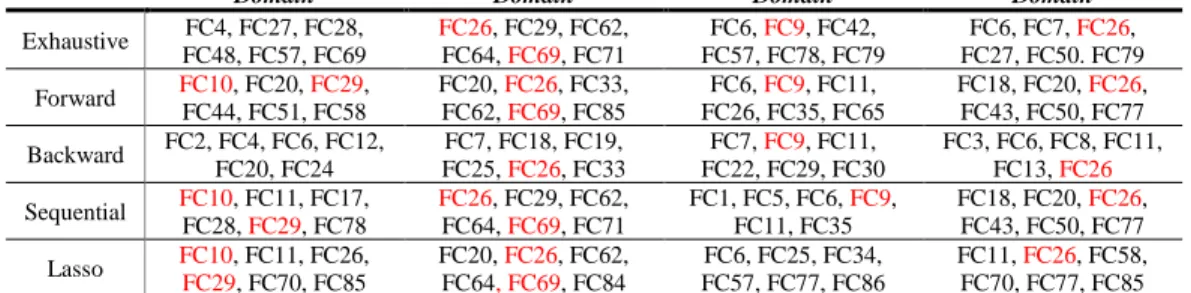
After we obtained the variable selection results from all the methods, we listed six of the selected variables in Table 2.4. For processing speed domain, “FC10” and “FC29” were selected frequently in all the five methods. For working memory domain, “FC26” was selected five times, which warrants more research on the network connectivity between the corresponding brain regions. “FC69” is the second frequent of all the selected variables. For episodic memory domain, “F9” is the most frequent variable with four times. For executive function domain, “FC26” are included in five methods, the same frequency for working memory domain. All the selected functional connectivity could be of future research interests

(36)

29

to explore the relationship between brain connectivity – cognition association and depression.

Table 2.4 Variable selection results from each method.

Processing Speed Domain Working Memory Domain Episodic Memory Domain Executive Function Domain Exhaustive FC4, FC27, FC28, FC48, FC57, FC69 FC26, FC29, FC62, FC64, FC69, FC71 FC6, FC9, FC42, FC57, FC78, FC79 FC6, FC7, FC26, FC27, FC50. FC79 Forward FC10, FC20, FC29, FC44, FC51, FC58 FC20, FC26, FC33, FC62, FC69, FC85 FC6, FC9, FC11, FC26, FC35, FC65 FC18, FC20, FC26, FC43, FC50, FC77 Backward FC2, FC4, FC6, FC12, FC20, FC24 FC7, FC18, FC19, FC25, FC26, FC33 FC7, FC9, FC11, FC22, FC29, FC30 FC3, FC6, FC8, FC11, FC13, FC26 Sequential FC10, FC11, FC17, FC28, FC29, FC78 FC26, FC29, FC62, FC64, FC69, FC71 FC1, FC5, FC6, FC9, FC11, FC35 FC18, FC20, FC26, FC43, FC50, FC77 Lasso FC10, FC11, FC26, FC29, FC70, FC85 FC20, FC26, FC62, FC64, FC69, FC84 FC6, FC25, FC34, FC57, FC77, FC86 FC11, FC26, FC58, FC70, FC77, FC85

(37)

30

SUMMARY AND FUTURE WORK

In this thesis, we developed a Bayesian hierarchical spatiotemporal model that combined fMRI and DTI data jointly to enhance the estimation of resting-state functional connectivity. Structural connectivity from DTI data was utilized to construct an informative prior for functional connectivity based on resting-state fMRI data through the Cholesky decomposition in a mixture model. The analysis took the advantages of probabilistic programming package as PyMC3 and next-generation Markov Chain Monte Carlo (MCMC) sampling algorithm as No-U-Turn Sampler (NUTS). The simulation study with this advanced algorithm, illustrated reduced mean squared errors (MSEs) of estimation. Furthermore, through a case study of MDD, we applied our model to examine how the estimated functional connectivity was associated with tasks of episodic memory, executive function, processing speed and working memory. Through five various methods of variable selection, certain estimated functional connectivity can be extended to investigate the correlated links between ROIs and depression in the future.

We have made significant progress in the development of estimating functional connectivity using PyMC3. However, abundant exciting opportunities are still available to further advance the capabilities and applications of our model. For example, we have listed a set of covariance function to capture local spatial correlation, which can be extended to compare the estimated results. Another explorable work is to combine all the variables including the covariates, estimated functional connectivity and multiple cognitive domains, and to build a classifier to identify whether this subject is under MDD or not. The case study in this thesis only have forty-one subjects, which is likely to be overfitted using the modern

(38)

31

machine learning techniques. For 200 ~ 300 subjects, multiple methods such as random forest, gradient boosting tree and support vector machine, can be applied to predict the classification of subjects or the value of cognitive domains.

In conclusion, we have proposed a Bayesian model for resting-state brain networks using the newly-developed probabilistic programming even though many challenges still exist. Hopefully, the work presented in this thesis will bring attention to future development of brain imaging.

(39)

32

APPENDIX

A.1 Setting of PyMC3 and Theano

The latest version of pymc3 package can be installed from PyPI using pip:

pip install pymc3

Or via conda-forge channel if you have installed Anaconda to manage installations of various packages:

conda install -c conda-forge pymc3

To mention, other related packages like numpy, pandas, theano will be installed together with pymc3. In addition, to ensure running pymc3 and theano in various OS systems such as Unix, Mac and Windows, other packages such as mkl-service and m2w64-toolchain

need to be installed with the underlined notices during the setup. For Windows users, environmental variables need to be added in the system setting to use conda command in the terminal and theano package in Python environment. C++ compiler such as Cygwin needs to be installed before running pymc3 and theano in Windows if it does not exist.

To use GPUs for intensive parallel computation purposes in theano on either Vanderbilt ACCRE or your own devices, a theanorc file is required and can be added based on theano GPU documentation or ACCRE python documentation in the GitHub pages. All the setting and examples are also illustrated in my GitHub repository named DoubleFusion (https://github.com/wangruinju/Double-Fusion).

(40)

33 A.2 Spatiotemporal Hierarchical Model in PyMC3

import numpy as np import pymc3 as pm import theano.tensor as tt import theano import csv import os

from datetime import date

def get_data(name):

yreader = csv.reader(open(name + ".csv"))

Y = np.array([row for row in yreader]).astype(float) return Y

def get_func(name, n):

sreader = csv.reader(open(name + ".csv"))

mFunc = np.array([row for row in sreader]).astype(float) func_new = np.array(mFunc[0, 0:n*(n-1)//2])

func_temp = np.triu(np.ones([n, n]),1) func_temp[func_temp==1] = func_new

Func_mat = func_temp.T + np.eye(n) + func_temp return Func_mat

def get_struct(name, n):

sreader = csv.reader(open(name + ".csv"))

S_read = np.array([row for row in sreader]).astype(float) struct_new = np.array(S_read[0:n*(n-1)//2, 0])

Struct_temp = np.triu(np.ones([n, n]), 1) Struct_temp[Struct_temp ==1] = struct_new

Struct_mat = Struct_temp.T + np.eye(n) + Struct_temp return Struct_mat

def get_dist(name, n): Dist = []

for i in range(1, n+1):

distreader = csv.reader(open(name + "_" + str(i) + ".csv")) Dist.append(np.array([row for row in distreader]).astype(float)) return Dist

def run_model(index, in_dir, out_dir, data_filename, func_filename, struct_file-name, dist_filestruct_file-name, n, sample_size, tune_size):

os.chdir(in_dir + str(index)) Y = get_data(data_filename)

mFunc = get_func(func_filename, n) Struct = get_struct(struct_filename, n)

(41)

34 Dist = get_dist(dist_filename, n) m = Dist[0].shape[0] k = Y.shape[1] n_vec= n*(n+1)//2 Y_mean = [] for i in range(n): Y_mean.append(np.mean(Y[i*m:(i+1)*m, 0])) Y_mean = np.array(Y_mean)

with pm.Model() as model_generator: # convariance matrix

log_Sig = pm.Uniform("log_Sig", -8, 8, shape=(n, )) SQ = tt.diag(tt.sqrt(tt.exp(log_Sig)))

Func_Covm = tt.dot(tt.dot(SQ, mFunc), SQ) Struct_Convm = tt.dot(tt.dot(SQ, Struct), SQ)

# double fusion of structural and FC

L_fc_vec =

tt.reshape(tt.slinalg.chole-sky(tt.squeeze(Func_Covm)).T[np.triu_indices(n)], (n_vec, )) L_st_vec =

tt.reshape(tt.slinalg.chole-sky(tt.squeeze(Struct_Convm)).T[np.triu_indices(n)], (n_vec, ))

Struct_vec = tt.reshape(Struct[np.triu_indices(n)], (n_vec, )) lambdaw = pm.Beta("lambdaw", alpha=1, beta=1, shape=(n_vec, )) Kf = pm.Beta("Kf", alpha=1, beta=1, shape=(n_vec, ))

rhonn = Kf*( (1-lambdaw)*L_fc_vec + lambdaw*L_st_vec ) + \ (1-Kf)*( (1-Struct_vec*lambdaw)*L_fc_vec + Struct_vec*lamb-daw*L_st_vec )

# correlation

Cov_temp = tt.triu(tt.ones((n,n)))

Cov_temp = tt.set_subtensor(Cov_temp[np.triu_indices(n)], rhonn) Cov_mat_v = tt.dot(Cov_temp.T, Cov_temp)

d = tt.sqrt(tt.diagonal(Cov_mat_v)) rho = (Cov_mat_v.T/d).T/d

rhoNew = pm.Deterministic("rhoNew", rho[np.triu_indices(n,1)]) # temporal correlation AR(1)

phi_T = pm.Uniform("phi_T", 0, 1, shape=(n, )) sigW_T = pm.Uniform("sigW_T", 0, 100, shape=(n, )) B = pm.Normal("B", 0, 100, shape=(n, ))

muW1 = Y_mean - B # get the shifted mean

mean_overall = muW1/(1.0-phi_T) # AR(1) mean

tau_overall = (1.0-tt.sqr(phi_T))/tt.sqr(sigW_T) # AR (1) variance

W_T = pm.MvNormal("W_T", mu = mean_overall, tau = tt.diag(tau_overall), shape = (k, n))

(42)

35

# add all parts together

one_m_vec = tt.ones((m, 1)) one_k_vec = tt.ones((1, k))

D = pm.MvNormal("D", mu=tt.zeros(n), cov=Cov_mat_v, shape = (n, )) phi_s = pm.Uniform("phi_s", 0, 20, shape = (n, ))

spat_prec = pm.Uniform("spat_prec", 0, 100, shape = (n, )) H_base = pm.Normal("H_base", 0, 1, shape = (m, n))

Mu_all_temp = [] for i in range(n):

# exponential covariance function

H_temp = tt.sqr(spat_prec[i])*tt.exp(-phi_s[i]*Dist[i]) L_H_temp = tt.slinalg.cholesky(H_temp)

Mu_all_temp.append(B[i] + D[i] + one_m_vec*W_T[:,i] + tt.dot(L_H_temp, tt.reshape(H_base[:,i], (m, 1)))*one_k_vec) MU_all = tt.concatenate(Mu_all_temp, axis = 0)

sigma_error_prec = pm.Uniform("sigma_error_prec", 0, 100)

Y1 = pm.Normal("Y1", mu = MU_all, sd = sigma_error_prec, observed = Y) with model_generator:

step = pm.NUTS()

trace = pm.sample(sample_size, step = step, tune = tune_size, chains = 1)

# save as pandas format and output the csv file

save_trace = pm.trace_to_dataframe(trace)

save_trace.to_csv(out_dir + date.today().strftime("%m_%d_%y") + "_sam-ple_size_" + str(sample_size) + "_index_" + str(index) + ".csv")

(43)

36 # initializing parameters index_list = [8007, 8012, 8049, 8050, 8068, 8072, 8077, 8080, \ 8098, 8107, 8110, 8146, 8216, 8244, 8245, 8246, \ 8248, 8250, 8253, 8256, 8257, 8261, 8262, 8263, \ 8264, 8265, 8266, 8273, 8276, 8279, 8280, 8282, \ 8283, 8284, 8285, 8288, 8290, 8292, 8293, 8295, \ 8299] in_dir = "/Users/ruiwang/source/doublefusion/simulation/data/" out_dir = "/Users/ruiwang/source/doublefusion/simulation/results/" data_filename = "ROI_timeseries_data" func_filename = "DMN_MeanFunctional_Connectivity" struct_filename = "DMN_StructuralConnectivity" dist_filename = "distMatrix_ROI" n = 14 sample_size = 1000 tune_size = 1000

# run the model

for index in index_list:

run_model(index, in_dir, out_dir, data_filename, func_filename, struct_file-name, dist_filestruct_file-name, n, sample_size, tune_size)

(44)

37

(45)

38 A.4 Regression Coefficients

Intercept Age sex Education FC_i Depress FC_i*Depress

1 1.17 -0.01 -0.00 -0.03 0.26 0.09 -0.53 2 -0.41 -0.01 -0.13 -0.03 2.80 3.19 -5.91 3 0.68 -0.02 -0.07 -0.02 1.00 1.05 -2.70 4 0.86 -0.02 -0.15 -0.01 1.07 -0.37 0.63 5 1.28 -0.01 -0.10 -0.04 0.75 -0.09 -0.10 6 1.18 -0.02 0.07 -0.02 0.83 -0.27 0.62 7 1.38 -0.02 0.05 -0.03 -0.15 -0.28 1.48 8 1.29 -0.02 0.02 -0.03 0.21 -0.14 0.44 9 1.12 -0.02 0.06 -0.02 -0.03 -0.08 1.00 10 0.60 -0.01 -0.08 -0.03 2.03 0.08 -0.47 11 1.09 -0.02 0.03 -0.01 -1.07 -0.10 0.06 12 1.05 -0.01 0.04 -0.02 -0.58 -0.08 1.37 13 1.66 -0.01 -0.08 -0.05 -1.08 -0.13 1.74 14 0.52 -0.02 0.02 -0.01 1.87 0.71 -3.25 15 -0.15 -0.02 -0.06 -0.01 2.72 2.23 -5.16 16 1.27 -0.02 0.03 -0.04 1.28 0.42 -3.23 17 1.59 -0.02 0.03 -0.04 -0.11 0.27 -1.52 18 1.25 -0.01 -0.01 -0.03 -0.04 -0.10 1.19 19 1.18 -0.01 0.04 -0.03 -0.93 -0.17 1.78 20 1.51 -0.02 -0.02 -0.05 -0.91 -0.09 0.50 21 1.35 -0.02 -0.01 -0.04 -0.54 -0.06 0.72 22 1.38 -0.01 -0.04 -0.04 0.14 -0.11 0.45 23 1.42 -0.02 0.01 -0.03 -0.27 -0.15 -0.02 24 1.40 -0.02 0.02 -0.03 -1.06 -0.24 1.38 25 1.50 -0.02 -0.05 -0.05 -1.44 -0.02 0.98 26 -0.66 -0.01 -0.10 -0.07 4.01 1.89 -3.44 27 1.05 -0.01 0.00 -0.04 0.74 0.56 -1.60 28 0.16 -0.00 -0.06 -0.05 3.24 1.10 -3.57 29 1.16 -0.02 -0.01 -0.02 0.36 -0.65 1.75 30 1.46 -0.02 0.01 -0.03 -0.66 -0.63 2.47 31 1.64 -0.02 -0.06 -0.05 0.98 -0.19 0.35 32 1.09 -0.02 -0.02 -0.02 -0.63 -0.10 2.11 33 1.05 -0.02 -0.04 -0.02 0.58 -0.62 1.37 34 1.37 -0.02 -0.00 -0.02 -1.32 -0.47 2.16 35 0.52 -0.01 -0.06 0.02 -1.39 -0.25 2.86 36 1.50 -0.02 -0.12 -0.03 -1.97 -0.17 3.12 37 1.29 -0.01 0.02 -0.04 0.47 0.63 -2.56 38 1.04 -0.01 -0.02 -0.04 0.84 0.49 -1.61 39 1.02 -0.02 0.06 0.00 -0.56 -0.63 2.31 40 1.28 -0.02 0.05 -0.02 -1.07 -0.49 1.89 41 1.43 -0.02 -0.03 -0.03 0.44 -0.16 0.70 42 1.49 -0.02 -0.03 -0.04 0.10 -0.12 1.47 43 1.33 -0.02 -0.00 -0.02 -0.67 -0.63 2.12 44 1.61 -0.02 -0.02 -0.02 -1.24 -0.23 0.64 45 0.91 -0.01 -0.01 -0.00 -0.65 -0.38 1.74 46 1.06 -0.01 -0.05 -0.02 -1.48 -0.02 2.21 47 -1.14 -0.01 -0.05 -0.06 4.07 3.51 -5.65 48 0.92 -0.02 -0.03 0.01 0.14 -0.42 2.16 49 1.12 -0.02 -0.01 -0.01 -0.25 -0.29 1.58 50 1.57 -0.01 0.03 -0.05 1.08 -0.11 -0.95 51 1.39 -0.01 -0.03 -0.04 -0.52 -0.12 -0.33 52 1.29 -0.02 -0.16 -0.03 1.14 -0.18 0.53 53 1.32 -0.02 -0.02 -0.02 -0.98 -0.22 1.44 54 1.20 -0.01 -0.00 -0.03 -0.25 -0.15 0.56 55 1.26 -0.02 -0.03 -0.02 -0.13 -0.06 1.44 56 0.90 -0.02 0.04 0.00 -0.24 -0.39 2.59 57 1.20 -0.01 0.02 -0.02 -0.41 -0.22 1.07 58 1.43 -0.01 0.04 -0.04 1.19 -0.17 -0.74 59 1.41 -0.01 -0.01 -0.04 0.19 -0.13 -0.05 60 1.38 -0.02 -0.10 -0.04 0.75 -0.11 0.15 61 1.68 -0.01 0.02 -0.04 -1.41 -0.26 0.64 62 1.50 -0.01 -0.06 -0.04 0.45 -0.10 -0.15 63 1.34 -0.02 -0.00 -0.03 0.67 -0.08 0.53 64 1.56 -0.01 -0.05 -0.04 -0.07 -2.47 3.56 65 1.39 -0.02 -0.05 -0.03 0.00 -0.33 1.66 66 1.41 -0.02 -0.11 -0.03 0.11 -0.29 1.85 67 1.53 -0.01 0.01 -0.03 -0.80 -0.60 1.22 68 1.51 -0.01 -0.02 -0.04 -0.45 0.08 -0.93 69 1.39 -0.01 -0.03 -0.04 0.09 -0.14 0.02 70 1.22 -0.01 -0.11 -0.02 1.96 -0.22 -0.11 71 1.44 -0.02 -0.05 -0.04 1.25 -0.07 -0.01 72 1.30 -0.02 -0.06 -0.02 0.22 -0.30 1.87 73 1.43 -0.02 0.06 -0.02 -1.46 -0.61 2.49 74 1.53 -0.02 0.01 -0.03 -0.98 -0.16 0.22 75 1.35 -0.01 -0.01 -0.03 -0.38 -0.14 0.62 76 2.08 -0.02 -0.19 -0.06 2.26 -0.21 -1.09 77 0.76 -0.01 -0.12 -0.04 1.08 -0.43 0.69 78 1.21 -0.02 -0.02 -0.02 -0.74 -0.19 2.62 79 1.07 -0.02 0.01 -0.02 -1.12 -0.04 2.58 80 2.31 -0.01 -0.01 -0.08 -2.82 -0.46 3.30 81 1.73 -0.02 -0.08 -0.04 -0.84 -0.63 2.30 82 1.56 -0.02 0.01 -0.04 0.98 -0.21 -0.14 83 1.53 -0.01 0.00 -0.05 0.54 -0.14 0.01 84 0.85 -0.01 0.07 -0.02 1.34 0.10 -1.38 85 1.00 -0.01 -0.00 -0.02 1.06 -0.03 -0.03 86 2.43 -0.01 0.12 0.00 -3.98 -2.86 6.38 87 1.58 -0.02 -0.05 -0.04 0.05 0.10 -1.80 88 0.40 -0.02 -0.01 0.03 0.78 -0.23 1.18 89 1.68 -0.02 0.06 -0.03 -1.32 -0.12 0.12 90 0.95 -0.01 -0.02 -0.01 0.20 -0.12 1.66 91 1.15 -0.02 0.00 -0.02 0.47 -0.06 -1.13 1

(46)

39

Intercept Age sex Education FC_i Depress FC_i*Depress

1 0.57 -0.03 -0.22 0.04 0.01 -0.68 1.31 2 0.80 -0.03 -0.06 0.06 -0.88 -2.60 4.33 3 0.97 -0.03 -0.10 0.04 -0.85 -1.81 3.77 4 0.20 -0.03 -0.12 0.08 -0.77 -0.68 1.78 5 0.29 -0.03 -0.09 0.07 -0.88 -0.47 1.37 6 -0.02 -0.04 -0.06 0.08 0.61 -0.37 1.06 7 0.26 -0.04 -0.08 0.07 0.80 -0.26 0.68 8 0.25 -0.03 -0.16 0.06 0.01 -0.16 -0.24 9 0.27 -0.03 -0.18 0.06 -0.15 -0.17 -0.29 10 -0.15 -0.03 -0.16 0.09 0.15 -0.46 0.99 11 0.00 -0.03 -0.10 0.08 -0.91 -0.30 1.32 12 0.00 -0.03 -0.12 0.08 -0.31 -0.13 0.78 13 0.02 -0.03 -0.10 0.08 0.59 -0.18 -0.25 14 0.28 -0.03 -0.16 0.06 -0.11 -0.24 0.34 15 0.38 -0.03 -0.14 0.07 -0.46 -0.03 -0.37 16 0.08 -0.03 -0.15 0.07 0.73 -0.00 -1.01 17 0.22 -0.03 -0.15 0.07 -0.07 -0.16 0.02 18 -0.01 -0.03 -0.16 0.08 0.30 -0.08 1.98 19 0.25 -0.03 -0.16 0.06 0.61 -0.17 -0.09 20 0.35 -0.03 -0.13 0.06 0.81 -0.33 -1.55 21 0.32 -0.03 -0.15 0.06 0.15 -0.23 -0.59 22 0.09 -0.03 -0.21 0.07 -0.81 -0.17 3.43 23 0.29 -0.03 -0.11 0.07 -0.62 -0.20 0.07 24 -0.06 -0.03 -0.16 0.08 0.02 -0.17 0.76 25 0.08 -0.03 -0.12 0.08 1.29 -0.28 -0.99 26 0.04 -0.03 -0.24 0.06 0.69 -1.36 2.08 27 0.13 -0.03 -0.12 0.06 0.28 0.46 -1.43 28 0.33 -0.03 -0.11 0.07 -0.31 0.04 -0.65 29 0.05 -0.03 -0.15 0.07 0.55 -0.31 0.47 30 0.18 -0.03 -0.15 0.07 0.09 -0.20 0.14 31 0.12 -0.03 -0.13 0.07 0.85 -0.15 -1.25 32 0.27 -0.03 -0.13 0.06 -0.05 -0.16 -1.00 33 0.24 -0.04 -0.13 0.10 -1.31 -1.10 2.66 34 0.35 -0.03 -0.18 0.08 -1.40 -0.32 1.26 35 -0.20 -0.03 -0.20 0.09 0.38 -0.17 0.60 36 -0.09 -0.03 -0.10 0.09 0.75 -0.22 0.13 37 0.26 -0.03 -0.13 0.07 -0.19 -0.08 -0.26 38 0.60 -0.03 -0.12 0.06 -0.87 -0.10 -0.18 39 0.18 -0.03 -0.15 0.07 0.06 -0.17 0.05 40 0.34 -0.03 -0.17 0.06 -0.13 -0.02 -0.62 41 0.34 -0.03 -0.15 0.06 0.73 -0.17 -1.14 42 0.37 -0.03 -0.17 0.06 0.41 -0.16 0.03 43 0.15 -0.04 -0.13 0.09 -0.89 -0.80 2.75 44 0.37 -0.03 -0.15 0.07 -0.86 -0.23 0.47 45 0.15 -0.03 -0.16 0.06 0.66 -0.11 -0.30 46 0.25 -0.03 -0.13 0.07 0.81 -0.21 -0.52 47 1.34 -0.03 -0.20 0.05 -1.18 -2.53 3.79 48 0.13 -0.03 -0.18 0.08 0.61 -0.21 0.18 49 0.16 -0.03 -0.15 0.07 -0.17 -0.19 0.40 50 0.50 -0.03 -0.11 0.04 1.47 -0.08 -2.74 51 0.36 -0.03 -0.17 0.06 0.57 -0.14 -0.97 52 0.08 -0.03 -0.19 0.09 -0.54 -0.48 2.44 53 0.33 -0.03 -0.12 0.06 0.07 -0.13 -0.57 54 0.56 -0.03 -0.17 0.05 0.52 -0.13 -1.06 55 0.20 -0.03 -0.10 0.07 0.65 -0.21 -0.81 56 0.48 -0.03 -0.18 0.04 0.12 -0.01 -1.50 57 0.48 -0.03 -0.14 0.04 -0.28 -0.03 -1.38 58 0.31 -0.03 -0.14 0.06 0.89 -0.17 -1.16 59 0.23 -0.03 -0.13 0.07 0.44 -0.14 0.35 60 0.36 -0.03 -0.19 0.06 -0.44 -0.39 2.16 61 0.22 -0.03 -0.13 0.06 0.14 -0.05 -0.87 62 0.18 -0.03 -0.21 0.07 0.27 -0.17 0.45 63 0.21 -0.03 -0.15 0.07 0.05 -0.17 -0.14 64 0.37 -0.03 -0.18 0.06 -0.10 -1.95 2.72 65 0.15 -0.03 -0.13 0.08 -1.04 -0.30 0.81 66 0.12 -0.03 -0.14 0.07 -0.61 -0.23 0.72 67 0.07 -0.03 -0.09 0.08 0.11 -1.17 2.48 68 0.26 -0.03 -0.15 0.07 -0.45 -0.16 -0.02 69 0.24 -0.03 -0.23 0.07 0.37 -0.17 0.26 70 -0.00 -0.03 -0.18 0.08 0.03 -0.18 1.05 71 0.19 -0.03 -0.14 0.07 -0.40 -0.20 0.25 72 0.15 -0.03 -0.13 0.08 -1.02 -0.29 1.11 73 0.18 -0.03 -0.11 0.08 -0.69 -0.51 1.73 74 0.32 -0.03 -0.12 0.08 -1.21 -0.31 0.81 75 0.19 -0.03 -0.15 0.07 -0.30 -0.16 0.47 76 0.40 -0.03 -0.21 0.06 0.57 -0.19 0.29 77 0.57 -0.03 -0.34 0.07 -0.61 -1.77 3.38 78 0.42 -0.03 -0.15 0.06 1.55 -0.15 -2.04 79 0.28 -0.03 -0.17 0.06 0.35 -0.21 -1.46 80 0.54 -0.03 -0.19 0.05 -0.48 -0.26 1.65 81 0.55 -0.03 -0.22 0.07 -0.77 -0.65 2.31 82 0.46 -0.03 -0.16 0.05 1.00 -0.19 -2.41 83 0.24 -0.03 -0.18 0.06 -0.04 -0.16 -2.05 84 0.09 -0.03 -0.13 0.07 0.30 -0.10 -0.32 85 0.47 -0.03 -0.20 0.07 -0.91 -0.45 2.14 86 1.20 -0.03 -0.09 0.07 -2.56 -1.08 1.96 87 0.21 -0.03 -0.17 0.07 0.31 -0.08 -0.70 88 -0.22 -0.03 -0.14 0.09 0.60 -0.17 0.04 89 0.54 -0.03 -0.10 0.07 -1.27 -0.33 0.91 90 -0.19 -0.03 -0.16 0.09 -0.36 -0.12 2.07 91 0.41 -0.03 -0.16 0.06 -0.37 -0.16 -0.30 1