University of Lethbridge Research Repository
OPUS http://opus.uleth.ca
Theses Arts and Science, Faculty of
2016
Testing the predictive power of various
exchange rate models in forecasting the
volatility of exchange
Obeng, Prince
Lethbridge, Alta : University of Lethbridge, Dept. of Economics
http://hdl.handle.net/10133/4611
TESTING THE PREDICTIVE POWER OF VARIOUS EXCHANGE RATE MODELS IN FORECASTING THE VOLATILITY OF EXCHANGE RATE
PRINCE OBENG
Bachelor of Arts, KNUST, 2012
A Thesis
Submitted to the School of Graduate Studies of the University of Lethbridge
in Partial Fulfillment of the Requirement for the Degree
MASTER OF ARTS
Department of Economics University of Lethbridge
LETHBRIDGE, ALBERTA, CANADA
TESTING THE PREDICTIVE POWER OF VARIOUS EXCHANGE RATE MODELS IN FORECASTING THE VOLATILITY OF EXCHANGE RATE
PRINCE, OBENG
Date of Defence: August17, 2016
Dr. Kien Tran Professor Ph.D. Co Supervisor
Dr. Duane Rockerbie Professor Ph.D. Co Supervisor
Dr. Alexander Darku Associate Professor Ph.D. Committee Member
Dr. Stavroula Malla Associate Professor Ph.D. Committee Member
Dr. Richard Mueller Professor Ph.D. Chair, Thesis Examination Committee
iii
Dedication
iv
Abstract
This Thesis tests the predictive power of ARCH, GARCH and EGARCH models in forecasting exchange rate volatility of Canadian dollar, Euro, British Pound, Swiss Franc and Japanese Yen using the US dollar as the base currency. We investigate both in-sample and out-of-in-sample performance of the volatility models using loss functions. The study further examines if the best model for the in-sample forecast will emerge as the best model for the out-of-sample forecast. The study finds that the GARCH(1,1) model outperforms all the other volatility models during the in-sample period. However in terms of the out-of-sample performance of the volatility models, the results are inconclusive, even though the ARCH model performed better most of the time than the complex models. The study concludes that the simple models should be given special consideration in terms of forecasting. Our results are robust to research on exchange rate volatility forecasting.
v
Acknowledgement
First and foremost, I am really thankful to the Almighty God for the gift of life, strength and knowledge bestowed on me to pursue this graduate degree. I wish to express my profound gratitude to my thesis supervisors Professor Kien Tran and Dr. Duane Rockerbie of the Department of Economics at the University of Lethbridge. The doors to Prof. Kien Tran and Dr. Duane Rockerbie were always open whenever I ran into trouble or had a question about my research. They consistently steered me in the right direction whenever I needed help. I am grateful for the unfailing patience, encouragement and valuable time they dedicated to the success of this thesis and my entire graduate degree.
I would like to express my sincere gratitude to my committee members, Dr. Alexander Darku and Dr. Starvoula Malla for their invaluable contribution to the completion of the thesis. I am most grateful to Dr. Darku for his encouragement, constructive criticism and time dedication throughout my entire graduate program. A special thanks to the faculty and staff of the Economics Department especially Dr. Richard Mueller, Dr. Kurt Klein, Dr. Pascal Ghanzalian, Jeff Davidson and Merle Christie.
I would like to express a special word of thanks to my colleagues and friends, Cosmas Dery, Richard Yeboah, Solomon Akowuah, Kwaku Adoo, Jessie Acquah, Frederick Amponsem, Frank Opoku, Innocent Kumah and last but not the least Prince Opoku Ware for their encouragement and support during my graduate studies. The love and encouragement of Nance Yaw together with the unwavering support of my mother, Mrs. Dorothy Asante has contributed to this height that I have achieved in the academic ladder.
vi Table of Contents CHAPTER ONE ... 1 1.1 Introduction ... 1 CHAPTER TWO... 13 2.1 Literature Review ... 13 CHAPTER THREE ... 21 3.1 Volatility Models ... 21 3.1.1 ARCH(p) ... 22 3.1.2 GARCH(p,q) ... 24
3.1.3 The Exponential GARCH ... 26
CHAPTER FOUR ... 28
4.1 ESTIMATION AND FORECASTING ... 28
4.1.1 Maximum Likelihood Estimation ... 28
4.2 Forecasting ... 30
4.2.1 Forecasting with ARCH (p) model ... 31
4.2.2 Forecasting with GARCH (p,q) model ... 33
4.2.3 Forecasting with the EGARCH(p,q) model ... 34
4.3 Forecasting using the Data ... 34
4.4 Model Selection ... 37
4.5 Forecast Evaluation ... 38
CHAPTER FIVE ... 41
5.1 Data and Results... 41
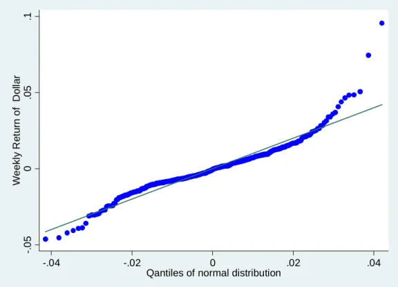
5.1.3 Jarque-Bera Test ... 48
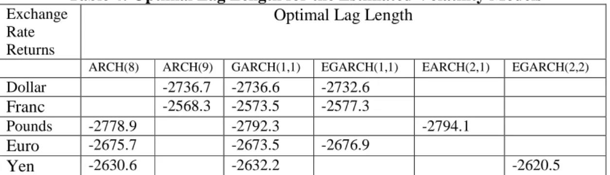
5.1 Model Selection for Forecasting ... 50
5.2 Evaluation of in-sample fit of the models. ... 52
5.3 Summary of the In-Sample performance of the Volatility Models ... 60
5.4 Evaluation of Out-of-sample forecast ... 61
CHAPTER SIX ... 72
6.1 SUMMARY CONCLUSION AND RECOMMENDATIONS ... 72
REFERENCES ... 76
APPENDIX A ... 80
APPENDIX B ... 81
APPENDIX C ... 82
vii
List of Tables
Table 1: Descriptive statistics of exchange rate returns ... 47
Table 2: Jacque-Bera test for CAN ... 49
Table 3: ADF test of exchange rate returns ... 50
Table 4: Optimal Lag Length for the Estimated Volatility Models ... 51
Table 5: MSE, R2LOG, MAD, and PSE values of In-Sample Forecasts ... 58
Table 6: MSPE,R2LOG, MAD and PSE values of Out-of-Sample Forecasts ... 61
viii
List of Figures
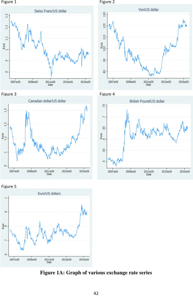
Figure 1A: Graph of various exchange rate series ... 42
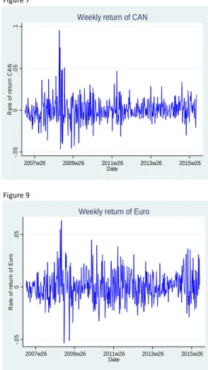
Figure 1B: Weekly return of the various exchange rate series ... 44
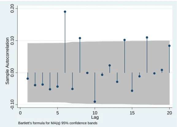
Figure 2: Sample Autocorrelation function for CAN ... 45
Figure 3: In-sample forecast of CAN... 53
Figure 4: In-sample forecast of Swiss Franc... 54
Figure 5: In-sample forecast of the BPS ... 55
Figure 6: In-sample forecast of the Euro. ... 56
Figure 7: In-sample forecast of Yen ... 57
Figure 8: Out-of-sample forecast of CAN ... 65
Figure 9: Out-of-sample forecast of Swiss Franc ... 67
Figure 10: Out-of-sample forecast of BPS... 68
Figure 11: Out-of-sample forecast of Swiss Franc. ... Error! Bookmark not defined. Figure 12: Out-of-sample forecast of Yen ... 70
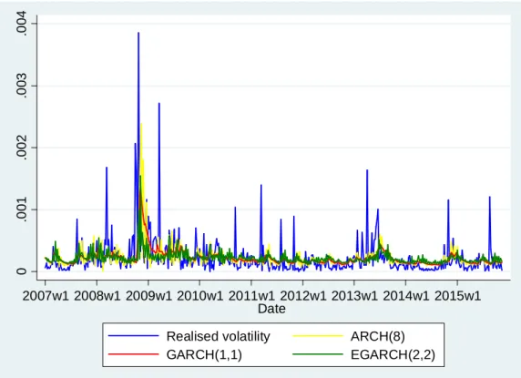
Figure 14: Realised volatility for the various exchange rate series ... 80
1
CHAPTER ONE
1.1 Introduction
Issues related to foreign exchange rate have always been the interest of researchers in modern financial theory because exchange rate, which is the price of one currency in terms of another currency, has a great impact on the volume of foreign trade and investment. Analysing the Forex market by volume shows that global daily Foreign Exchange transactions exceeded $4 trillion in 2010 which is bigger than the annual value of global trade (Bank for International Settlement, 2010). It is therefore not surprising that stable exchange rate has served as a catalyst for economic growth for most developed countries (countries which produce for export) whereas a highly volatile exchange rate is a major problem for most developing countries (developing countries who are import dependent).
The huge volume of transactions in the forex market makes it difficult for one to examine global interaction among countries with little or no understanding of the driving forces of exchange rates. In addition to that, the forex market is also an extremely nonlinear vibrant system which performance is influenced by a number of factors, namely inflation rates, interest rates, economic atmosphere, political issues, and many other factors. Hence forecasting the exchange rate index is challenging and a tricky issue for both for investors and academics (Sutheebanjard and Premchaiswadi, 2010).
The post Bretton Woods exchange system has seen substantial and growing literature on testing the predictive power of models used for forecasting foreign exchange rates movements. Reasons put forward for the intense research in this topical area are that,
2
accurate forecasts of exchange rate volatility can signal an early warning to a government of an upcoming economic crisis, and thereby aids policy makers to design and implement appropriate exchange rate policies to mitigate the anticipated economic turmoil. Similarly, accurate exchange rates volatility forecast is an important decision instrument that guides the choice of an exchange rate regime that is best for a particular country (Hernandez and Montiel, 2001) and can signal the optimality of a monetary union (Wyplosz, 2002). Ogawa (2002) posits that forecasting high exchange rate volatility in countries with flexible exchange rate regimes can influence the countries to enter a common exchange regime system as it is said to promote economic stability.
According to Antonakakis (2007), increase knowledge of the behaviour of the exchange rate does not only benefit the governments of countries but also the Central banks. His study asserts that, the Central banks rely on internal forecasts of exchange rate volatility to ascertain whether an exchange rate will fluctuate within or outside a target zone. Thus, exchange rate forecast in excess of the target rate will necessitate the intervention of the central bank, some of which include inflation targeting, interest rate targeting and other controls. The research by Antonakakis (2007) also posits that accurate knowledge of exchange rate forecasting is important for international traders’ export and import decisions because forecasting excessive exchange rate volatility in a country, ceteris paribus, will have a different impact on traders as it will make risk-averse traders reduce the volume of their transactions with such a country because of the uncertainty of their profits. However, risk-lover traders who trade on risk could benefit from seeking out hedging opportunities.
3
Accurate volatility forecasting of exchange rate also guides the decisions of investors, especially international investors who require portfolio diversification beyond national borders, or risk managers using internal models such as value-at-risk applications. International investors and risk managers have certain levels of risks that they can bear, so an accurate forecast of exchange rate volatility over the investment holding period serves as a good starting point for assessing their investment risk. As far as a risk-averse investor is concerned, uncertainty is the most important factor in pricing any financial asset. Hence most asset pricing theories try to model this uncertainty or risk by using the covariance between asset return and the market portfolio. Although it has been recognized for quite some time that the uncertainty of speculative prices, as measured by the variance and covariance, is changing through time, it is not until recently that researchers have started to explicitly model this time variation in second or higher order moments. This breakthrough in the area of volatility modeling confirms that accurate forecast of large exchange rate volatility has greatly affected the decision making process of highly risk-averse as opposed to risk-neutral investors. In addition, risk managers who want to minimize risks and are aware of accurate forecasts of large exchange rate volatility in a country, can still hold assets denominated in that country’s currency by investing in a second country’s currency, where exchange rate volatility is equally large but negatively correlated with that in the former country. This negative correlation could help offset risks. Accurate volatility forecasts therefore act as an input in their portfolio diversification and risk management (Antonakakis, N. 2007). In conclusion, a continuous improvement in forecasting accuracy will no doubt have substantial benefits for the various groups of agents since their decision making will be better informed. In contrast,
4
the costs of generating poor forecasts are substantial, as their decision making will be flawed and have unanticipated effect on the global economy.
Notwithstanding the importance of forecasting exchange rate volatility, theories of forecasting volatility of exchange rate has been in existence for many centuries with different models yielding different forecasting results either in-sample or out of sample data. The traditional financial economics research on exchange rate volatility has focused on the mean of exchange rate returns but in recent times the emphasis on mean retuned of exchange rate has shifted to the volatility of the exchange rate. Also the international stock market crash of 1987 has further increased the focus of regulators, practitioners and researchers on forecasting the volatility of exchange rate (Brailsford, 1995). As a result, some researchers have employed multivariate regression approach to study and predict the exchange rate volatility based on macroeconomic variables. Several others have also relied on structural models to predict the volatility of exchange rate, but these approaches have limitations in the sense that there are generally weak relationships between exchange rate and virtually any macroeconomic variable a situation commonly known as the “exchange rate disconnect puzzle” (Obstfeld et al., 2000). Also Flood et al., (1995), observes that nominal exchange rates are much more volatile (at low frequencies) than the macroeconomic variables which determines exchange rate theoretically hence this excess volatility associated with exchange rate makes structural models unsuccessful in forecasting exchange rate volatility. Cheung, Chinn and Pascual (2002), provides a survey of the literature on forecasting exchange (conditional mean) based on macro fundamentals. The study fails to identify papers with good predictive power that are able to overcome the random walk model. Also following the seminal paper of Meese and
5
Rogoff (1983), many tests have been done in search of macroeconomic models that have good power for forecasting movements but prove futile. These limitations associated with macroeconomic variables and structural models in predicting exchange rate volatility have led some researchers to ask the question that “why not exchange rate explains itself?”. That is with the little information on exchange rate, it should be able to forecast its current as well as future volatility by using robust time series or technical model (Onasanye et al., 2013). Nevertheless, the uncertainty of the exchange rate continues to present a challenge for economic agents to determine the directionality of the actual or future volatility of exchange rate. This is because the more forecast errors economic behaviors make in predicting the directionality of exchange rate volatility, the higher the trends in the uncertainty of the exchange rate are shown (Yoon et al, 2008).
Forecasting volatility of financial assets continues to occupy a center stage in research (Longmore and Robinson 2004). However, variance or standard deviation which is the traditional measure for volatility is unconditional and does not recognize the patterns in asset volatility such as time-varying and clustering properties. Researchers have therefore introduced various models to explain and predict these patterns in volatility. Engle (1982) is the first to introduce the autoregressive conditional heteroscedasticity (ARCH) to model volatility. The ARCH, models the heteroscedasticity by relating the conditional variance of the disturbance term to the linear combination of the squared disturbances in the recent past. Bollerslev (1986) generalizes the ARCH model by modeling the conditional variance to depend on its lagged values as well as squared lagged values of disturbance, and he calls this model generalized autoregressive conditional
6
development of financial econometrics in the past two decades. The GARCH model is useful for interpreting the volatility-clustering effect, which is an important facet of asset prices (Mandelbrot, 1963). Volatility clustering means that large changes of an asset’s price are followed by large changes in either sign. The model is also useful for many financial applications, such as measuring volatility of financial markets, pricing options, and computing Value at Risk (VAR) (Engle, 2002). Engle (1982) notices that although OLS (Ordinary Least Square) maintains its optimality properties when it is used to forecast exchange rate volatility, however, the parameters of ARCH models provides a better estimate when maximum likelihood method is employed. Similarly, Lastrapes (1989) complements the work of Engle when he observes that ARCH provides a better explanation of exchange rate process and it is consistent with exchange rates behaviour. Zivot (2009) also provides an in-depth empirical analysis of GARCH models for financial time series with emphasis on practical issues associated with model specification, estimation, diagnostics, and forecasting and finds the GARCH model to
provide better description of financial data compared to the OLS. According toBala et
al., (2013) the GARCH model has dominated the literature on volatility since the early 1980s because the model allows for persistence in conditional variance by imposing an autoregressive structure on squared errors of the process. This indicates that the superiority of the ARCH/GARCH models over other models in forecasting exchange rate volatility has contributed to its entrenched position and success in the forecasting literature.
Since the work of Engle (1982) and Bollerslev (1986), various forms of GARCH model have also been developed to model volatility. Some of the models include Integrated
7
GARCH (IGARCH) originally proposed by Engle and Bollerslev (1986), GARCH in- Mean (GARCH-M) model introduced by Engle, Lilien and Robins (1987),the standard deviation GARCH model introduced by Taylor (1986) and Schwert (1989), the Exponential GARCH model (EGARCH) proposed by Nelson (1991), Threshold ARCH (TARCH), and the Threshold GARCH have been introduced independently by Zakoïan (1994) and Glosten, Jaganathan, and Runkle (1993), the Power ARCH model generalised by Ding, Zhuanxin, C. W. J. Granger, and R. F. Engle (1993) etc.
Recently, the observance of volatility breaks in time series data has paved way for volatility models which allow for volatility breaks, a typical example is the Markov– switching models of conditional heteroscedasticity (see Lange and Rahbek, 2008). In view of that, Hammoudeh and Li (2008) have analysed sudden changes in volatility for five Gulf area stock markets and find that accounting for the large shifts in volatility in the GARCH (1,1) models reduces the estimated persistence of the volatility of the Gulf stock markets significantly.
Notwithstanding the vast aforementioned models in forecasting the volatility of exchange rate, other research work indicate that the behavior of dealers and other market participants can influence fluctuations in exchange rates (Lyons and Evans, 2002; Covrig and Melvin, 1998). Inventory adjustments and bid–ask spread reactions to informative incoming order flows are some of ways by which dealer behavior affects exchange rate determination and volatility. Also different market participants depend on both private and public information sets; hence it is natural to assume that equilibrium exchange rate expectations are formed based on a combination of macroeconomic fundamentals and market microstructure variables (Goldberg and Tenorio, 1997). Moreover, it is most
8
likely that the macroeconomic information and order flow information are processed in a nonlinear fashion. In line with this thinking, Gradojevic et al. (2006) apply the (Artificial Neural Network) ANN model to forecast high-frequency Canadian/US dollar exchange rate.
1.2 Thesis Objectives
Despite the different models that have evolved to forecast exchange rate volatility, large swings in price movements has become more prevalent and observers have damned institutional changes for this increase in volatility. These concerns have led researchers to analyse the level and stationarity of volatility over time. Specifically, research have been directed toward examining the accuracy of volatility forecasts obtained from various econometric models including the autoregressive conditional heteroscedasticity (ARCH) family of models. Interestingly, research conducted in the area of comparing volatility models are very limited. Also empirical research aim at comparing volatility models using at most three currencies and most of the time ignore the vehicle currencies in the world.
However, given the important role that exchange rate plays in each economy and the challenge in explicitly rating one volatility model over the other, this thesis examines the predictive power of various exchange rate models for six major trading currencies (Canadian dollar, US dollars, British pounds, Euro, the Japanese Yen, and Swiss franc).
Specifically, the study will
1. Provide extensive development of each model
9
3. Test the out-of-sample performance of the ARCH, GARCH and EGARCH model.
Various models have been used to forecast the volatility of exchange rate. However, researchers have not reached a consensus as to which model is better than the other in terms of exchange rate volatility forecasting. It is against this background that the purpose of this research is unique as it seeks to test the predictive power of various ARCH/GARCH (Generalised Autoregressive Conditional Heteroscedasticity) type models which include ARCH(p,q), GARCH(p,q) and EGARCH(p,q) to forecast exchange rate volatility in the context of six major trading currencies in the world (Euro, Canadian dollar, the Great British Pound, the Japanese Yen and the Swiss franc). The US dollar is used as the base currency against which all the other currencies are compared.
Adamu (2005) for example examines the impact of exchange rate volatility on private investment using GARCH type models and confirms an adverse effect of exchange rate volatility on private investment. Mordi (2006) employing GARCH model argues, that failure to properly manage exchange rates can induce distortions in consumption and production patterns. The study concludes that; excessive currency volatility creates risks with destabilizing effects on the economy. Hence a study that compares the predictive power of volatility models will contribute immensely to the smooth running of the global economy.
The study compares the ARCH family model which is at the core of volatility modelling with other extensions of volatility models in order to ascertain whether the basic models should be repudiated during forecasting exchange rate volatility since available literature advocate for complex models in forecasting volatility.
10
1.3 Thesis Contribution
Forecasting volatility and determinants of exchange rate have been well established in the literature. Efforts have been made to compare the performance of volatility models in forecasting exchange rate at various forecasting horizons. Also noted in the literature is the evaluation of the forecasting performance of volatility models in a particular family. Almost all the empirical research are either limited in the number of currencies used or focus on estimating the forecasting performance of volatility models at various forecasting horizons. An area which has witnessed less quantitative research is the evaluation of the forecasting performance of various exchange rate models from different family of volatility models. Hence the main objective of the thesis is to assess the forecasting performance of various exchange rate models in forecasting the volatility of exchange rate. This will help assess whether the simple models like the ARCH are able to perform better than the complex models or not. Most of the time research are directed towards assessing the performance of complex exchange rate volatility models with little or no reference to the simple models for forecasting exchange rate volatility. However as noted by Dimson and Marsh (1990), the simple models cannot be overlooked in forecasting volatility of exchange.
The thesis compares the forecasting performance of volatility models across six vehicle currencies in the world (Euro, Canadian dollar, the Great British Pound, the Japanese Yen and the Swiss franc). Previous studies have investigated only a limited range of exchange rates volatility between different currencies. Hence the use of six major currencies serves as an extension of previous studies. This also makes study particular of interest against the background that these six currencies are the world’s most heavily traded currencies, a
11
fact which cannot be explained by economic size alone. Furthermore, these currencies are characterised by a relatively high degree of speculative activity and a significant and highly variable amount of interventions by their monetary authorities. This study therefore assesses the performance of the volatility models notwithstanding the monetary control of the respective countries.
The study contributes to available literature by employing current data set and extensively developing the volatility models used in the study. With the passage of time the evolution of volatility may change, hence the use of current data set which spans the period where the world has witnessed the greatest financial crisis of the time will be literature enriching. Unlike other empirical studies which just state the volatility model to be compared, this study extensively develop each model to be used for forecasting which contributes to clear understanding of the subject matter of the thesis.
1.4 Thesis Organisation
This thesis is organized as follows: Chapter 2 provides a detailed discussion of empirical studies on exchange rate forecasting exchange rate volatility. Chapter 3 provides extensive development of the forecasting models. Chapter 4 provides estimation and forecasting with the various models, distributional assumptions of the volatility models and how the data are used for forecasting both in-sample and out of sample. It also presents how the models for comparison are going to be selected and also discusses the forecast evaluation of each model. Chapter 5 presents data and discusses the empirical results while summary, recommendation and concluding remarks are presented in Chapter 6. Appendix A describes the realized volatility for the various exchange rate
12
series. Appendix B contains the sample autocorrelation for the various exchange rate series and Appendix C describes the selection of the models for forecasting using AIC.
13
CHAPTER TWO 2.1 Literature Review
Predicting exchange rate volatility is difficult task. Despite the large body of research on exchange rate modeling, a key popular fact in international finance is that the best prediction for tomorrow’s exchange rate is today’s rate (known as the “random-walk forecast”). This result is first discovered by Meese and Rogoff (1983a, b) and after 25 years later, only few models could do better than random walk. A related result, also found in the literature by Hansen et al. (1980) indicates that the forward rate does not provide the best prediction for tomorrow’s exchange rate. Clarida et al., (2003) reaffirms the proposition of Hansen et al., (1980) as he notes that “from the early 1980s onwards, exchange rate forecasting is a difficult task because of the uncertainty associated with its forecast. The uncertainty associated with exchange rate forecast has made forecasting exchange rate increasingly come to be seen as a hazardous occupation and hence using the random walk model is the best specification for modeling exchange rate volatility.
A good review of the theories that have dilated on the exchange rate variability can be found in the research work by Cheung, Chinn and Pascual (2002). These authors use different approaches to study exchange rate volatility and they test the predictive power of four exchange rate models for the exchange rates series of Canada, Britain, Germany, Switzerland and Japan using the U.S. dollars as a base currency. The models tested in their works include stick-price monetary model, in line with Dornbush-Frankel, Balassa-Samuelson, which considers productivity differentials among countries, Behavioral Equilibrium Exchange Rate (BEER), which incorporates features of a wide range of models; and Unconvered Interest Rate Parity. Their studies find that, none of the tested
14
models outperforms the random walk model in forecasting the exchange rate volatility using the criterion of mean squared error. However, their studies conclude that on a longer horizon, structural models on the average provides a higher forecasting performance than the random walk model.
Since the seminal works of Mandelbrot (1963a, 1963b, 1967) and Fama (1965), researchers have found that the characteristics of the foreign exchange returns are non-linear, exhibits temporal dependence, and the distribution of exchange rate returns are leptokurtic (Friedman and Vandersteel (1982), Bollerslev (1987), Diebold (1988), Hsieh (1988, 1989a, 1989b) Diebold and Erlove (1989), Baillie and Bollerslev (1989)). Their researches also find that both large and small changes in returns are ' clustered' together over time, and the return distribution of the data used are bell-shaped, symmetric and fat-tailed. Data with such characteristics are captured well by Autoregressive Conditional Heteroskedasticity (ARCH) model introduced by Engle (1982) and the Generalised ARCH (GARCH) model developed by Bollerslev (1986).
However, the ARCH model is first used to model the currency exchange rate by Hsieh (1989a). The study investigates whether daily changes in five major foreign exchange rates contain any nonlinearity. The research concludes that although the data contains no linear correlation, however there is the presence of substantial nonlinearity in a multiplicative rather than additive form. The study then suggested that the generalized ARCH (GARCH) model can offer explanation to a large part of the nonlinearities for all five exchange rates. Since then, applications of these models to currency exchange rates have increased tremendously, with studies like Hsieh (1989b), Bollerslev (1990), Pesaran et al. (1993), Copeland et al. (1994), Takezawa (1995), Episcopos et al. (1995), Brooks
15
(1997), Hopper (1997), Cheung et al. (1997), Laopodis (1997), Lobo et al. (1998) and Duan et al. (1999). In most of the applications of the ARCH model, it is found that a very high-order ARCH model is required to model the changing variance. The alternative and more flexible lag structure is the Generalised ARCH (GARCH) introduced by Bollerslev (1986). Bollerslev et al., (1992) indicates that the squared returns of not only exchange rate data, but all speculative price series, typically exhibit autocorrelation and that large and small error tend to cluster together in continuous time periods in what has come to be known as volatility clustering.
Amidst the difficulty in forecasting the exchange behavior, Lam et al., (2008) compares five structural models (the PPP (Purchasing Power Parity) model, the UIP (Uncovered Interest Parity) model, the SP(semiparametric) model, the BMA (Bayesian Moving Average) model) and the composite (specification incorporating the above four models) model to the random walk model in predicting exchange rate behaviour in Hong Kong. The research uses the mean- square errors to determine the predictive power of the models and concludes that, the structural models are able to outperform the random walk model in certain time horizons but the combined forecast model has the best predictive power as it dominates all the models compared.
Similarly, Dan Bianco et al (2012) construct fundamentals-based econometric model for the weekly changes in the euro-dollar rate between 1999-2010 to forecast both the short run and the long run exchange rate between the euro and the dollar. The research further tests the predictive power of this model against the random walk model using mean square prediction error and a non-parametric test of predictive performance developed by Pesaran and Timmermann (1992). The research finds statistically significant
16
improvements upon the hard-to-beat random walk model using traditional statistical measures of forecasting error at all horizons. Also the study employs Direction of Change (DCH) measure, which evaluates out-of-sample forecasts by comparing the sign of the forecasts with the sign of the true observation. This test also complements the predictive power of the economic model against the hard to beat random walk model.
In a similar vein, Groen (2005) tests the a long-run link between monetary fundamentals, the Euro, exchange rates of Canada, Japan, and the United States and finds out that there exist a strong link between the monetary fundamentals and the long run exchange rate of the countries involved. The research further tests the out-of-sample performance of the model with the random walk model and finds out that, the model is superior to the random walk using the cointegrated VAR (Vector Autoregressive) model-based forecasts, especially at horizons of 2 to 4 years.
Gradojevic et al. (2006) applies the ANN (Artificial Neural Network model) model to forecast high-frequency Canadian/US dollar exchange rate. This is the first time microstructure variable is applied to forecast Canada/US exchange rate. The research concludes that the introduction of the microstructure variable improved both the linear and nonlinear models of exchange rate. The research further employs the Root mean square error prediction to the test the predictive power of the model and concludes that the ANN model is consistently better than the random walk and other linear models for the various out-of-sample set sizes.
Andersen and Bollerslev (1998a) have examined the DM/USD (Deutsh mark/US dollar) intraday volatility based on a year sample of five minutes returns with emphasis on
17
activity patterns, macroeconomic announcement and calendar effects. The study reveals that market activity is correlated with price variability. Hansen and Lunde (2005) compare 330 ARCH–type models in terms of their ability to describe the conditional variance, and finds no evidence that a GARCH (1,1) model is outperformed by more sophisticated models in their analysis of exchange rates. However, Teräsvirta (2009) reviews several univariate models of conditional heteroscedasticity and reports that GARCH models tend to exaggerate volatility persistence.
Kasman et al. (2011) investigates the relationship between interest rate and exchange rate changes on Turkish bank’s stock returns and finds significant negative association. Their results further reveal that interest and exchange rate volatility are the major determinants of conditional bank stock return volatility.
In assessing the performance of volatility models in the in-sample, Taylor (1987) and more recently West and Chow (1995) examine the forecast ability of exchange rate volatility using a number of models including ARCH. The study considers five U.S. bilateral exchange rate series. They find that generalised ARCH (GARCH) models are preferable at a one-week horizon, whilst for less frequent data, no clear victor is evident. Some other studies which tested the forecasting ability of volatility models in the in-sample include Meese and Rose 379 (1991), McKenzie (1997), Christian (1998), Longmore and Wayne Robinson (2004), Yang (2006) Yoon and Lee (2008) among others.
It is quite surprising that the available literature concentrates on in-sample forecast of exchange rate volatility with little emphasis on out-of-sample forecast. The few papers
18
that have tested the forecasting ability of ARCH/GARCH models in the out-of-sample have reached mixed results. Akgiray (1989), finds that a GARCH (1,1) specification exhibits superior forecasting ability of weekly US stock market volatility compared to more traditional models. However, Tse (1991) and Tse and Tung (1992) reach a different conclusion on the superiority of the GARCH model in the Japanese and Singaporean markets, respectively. Their studies find evidence strongly in favour of an exponentially weighted moving average (EWMA) model. In an examination of the UK equity market, Dimson and Marsh (1990) conclude that simple models provide more accurate forecasts, and hence the study recommends the exponential smoothing and simple regression models. However, Dimson and Marsh did not subject ARCH models to examination. Nevertheless, the conclusions of Dimson and Marsh have important implications for forecasts obtained from the relatively complex GARCH model as their research finally concludes that with the increase interest in using complicated econometric techniques for volatility forecasting, their research bet to differ from the status quo. That implies that those who are interested in forecasts with reasonable predictive accuracy, the best forecasting models may well be the simplest ones (Dimson and Marsh, 1990).
Also Hansen et al. (2005) compare 330 ARCH-type models in terms of their ability to
describe the conditional variance. The models are compared based on their out-of-sample performance using DM/USD (Deutsche Mark/US Dollars) exchange rate data and IBM return data. The study finds no evidence that a GARCH(1,1) is outperformed by more sophisticated models in the analysis of exchange rates. However, the GARCH(1,1) model is found inferior to models that can accommodate a leverage effect in the analysis of IBM returns. The study also employs the test for superior predictive ability (SPA) and the
19
reality check for data snooping (RC) to compare the models’ predictive power. The empirical results show that the RC lacks power to an extent that makes it unable to distinguish ‘good’ from ‘bad’ models in their analysis.
In forecasting exchange rate volatility between Naira and US Dollar, the Statistics Unit of Usmanu Danfodiyo University (2014), investigates the volatility modeling of daily Dollar/Naira exchange rate using GARCH, GJR-GARCH, TGARCH and TS-GARCH() models and daily data over the period June 2000 to July 2011. The results show that the GJR-GARCH and TGARCH models exhibit the existence of statistically significant asymmetry effect. The research further examines the forecasting ability of the models using the symmetric lost functions which are the Mean Absolute Error (MAE), Root Mean Absolute Error (RMAE), Mean Absolute Percentage Error (MAPE) and Theil inequality Coefficient. The results show that TGARCH model provide the most accurate forecasts because it captures all the necessary stylize facts (common features) of financial data, such as persistent, volatility clustering and asymmetric effects.
Bonilla et al (2003) apply the Hinich portmanteau bicorrelation test to find out the suitability of using GARCH (Generalized Autoregressive Conditional Heteroscedasticity) as the data-generating process to model conditional volatility of stock market index rates of return in 13 emerging economies. The study finds that a GARCH formulation or any of its forms fail to provide an adequate description for the underlying process of the 13 emerging stock market indices. The study also examines the existence of ARCH effects, over windows of 200, 400 and 800 observations, using Engle’s LM (Lagrange Multiplier) test, and find no evidence to support the existence of ARCH effects over long periods of time. The results of the study also hints that policymakers should exercise caution when
20
using autoregressive models for policy analysis and forecast because of the failure of the GARCH models to efficiently model the data generating process of the stock indices. The failure of the GARCH to model the stock indices has strong implications for the pricing of stock index options, portfolio selection and risk management. The study finally concludes that in analysing spillover effects and output volatility the GARCH model will not be efficient and hence cannot be used to evaluate economic policy in this direction. Will the same conclusion be reached when the GARCH model is used to forecast exchange rate volatility?
21
CHAPTER THREE 3.1 Volatility Models
The volatility models that is estimated in this study include ARCH(p), GARCH(p,q) and EGARCH(p,q). According to Tsay (2005), differences in volatility models are due to the way variance evolves over time. Conditional heteroscedastic models can therefore be classified into two groups. The first group uses exact functions to govern evolution of
variance() , while the second category uses stochastic equations to describe .
ARCH/GARCH models belong to the first category whereas stochastic volatility models belong to the second category (Tsay, 2005). This study therefore adopts a family in the first group where an estimated volatility model is used to examine volatilities in the six exchange rate series under investigation. We choose the ARCH/GARCH models because of the limitation of the ordinary least square.
A major assumption behind Ordinary least square is that the expected value of all errors terms when squared is the same at any given point or constant variance (a property of OLS commonly known as homoscedastic). If this condition is violated, then the Ordinary least square estimates for the coefficients will not have minimum variance even though the coefficients will still be unbiased estimates. However, the standard error and confidence intervals calculated in this case become too narrow, giving a false sense of precision. The ARCH/GARCH models handle this problem by modeling volatility to depend on previous volatility in the regression equation and thereby correcting the
deficiencies of least squares model.The ability of the ARCH model to capture volatility
clustering and the fact that it is mean reverting makes it a preferred model over other models which fail to capture these important features of time series data.
22
The GARCH model is a generalization of the ARCH model and it contains the ARCH
model as a special case. The GARCH model has an added lagged conditional variance
to prevent adding many lagged squared returns as is the case of the ARCH model. The GARCH(p,q) can be explained in a context where a currency trader predicts this period’s variance by forming a weighted average of a long term average (the constant), the forecasted variance from last period (the GARCH term), and information about volatility observed in the previous period (the ARCH term). If the asset return is unexpectedly large in either upward or downward direction, then the trader will increase/decrease his estimate of next period’s variance. There are some limitations of the GARCH(p,q) model since the model places restriction on the coefficients. The non-negativity conditions on can be violated by the estimation method, since the coefficients of the model can be negative. This limitation of the GARCH model influenced the consideration of another volatility model called the Exponential GARCH (EGARCH) model proposed by Nelson (1991). The EGARCH model eliminates the restriction that the GARCH model imposes on its parameters. The EGARCH model also allows for asymmetric effects between positive and negative asset returns and is a slight modification of the GARCH(p,q) model. This model has been proposed to solve the GARCH model’s failure to capture the asymmetric effects of positive and negative asset returns.
3.1.1 ARCH(p)
Let be the return on exchange rate. In a standard linear regression, the ARCH model
according to Engle, (1982) and Tsay, (2005), is characterized by mean and volatility equations, which are specified as:
23
where is the information set up to t-1 and ⎸ = (⎸)
⎸ is a conditional mean of , which is a function of the information set containing
all relevant information up to time − 1. The conditional variance at time t, that is ⎸
is defined as the expectation of the squared process in deviation from its mean:
⎸ =
− ⎸⎸ = (⎸) (2)
If the conditional mean ⎸ is zero which is a common feature of the financial returns,
then the conditional variance becomes ⎸ = (⎸) . To model the variance
efficiently, an important characteristic of the error term and the conditional variance
must be noted. The error term is conditionally heteroscedastic because the conditional
variance is time varying. We assume that the error term is multiplicative as in =
⎸ with being an independent and identically distributed innovation with
() = 0 and () = 1. The assumption on is consistent with the definition of the
conditional variance. Hence by taking conditional expectation of following an ARCH
process of order p, (ARCH(p)) is given by:
(⎸) ≡ − ⎸⎸ = ⎸ ⎸ = ⎸ (⎸) =
⎸ (3)
= + + + ⋯ !! (4)
where we have used the law of iterative expectation in equation (4). From equation (4),
the dependent variable is and there are p autoregressive terms , ……….! .
24
magnitude of the previous surprises # for $= 1, 2 ….p. Because # is squared, the
sign of the surprise is irrelevant; only the magnitude. This specification makes sense if we think that “surprises” are the source of uncertainty, which is at the heart of volatility.
To obtain the conditional variance of equation (3), the values of #s need to be estimated.
For the conditional variance to be positive, > 0, # ≥ 0 ∀$ .Also we assume that the
conditional mean ⎸ is constant over time hence we concentrate on modeling of the
conditional variance of the stochastic process that is equation (4). To be able to fit the
model to the data, the order of p needs to be specified. The order of ( in the ARCH
model can be determined by using either the AIC or the Sample Partial Autocorrelation function (PACF) of the squared returns where the Sample PACF is not significantly different from zero for lags greater than p. Research has shown that the ARCH model requires a high order to be able to accurately model conditional variance (see Hansen and Lunde (2005) and Bollerslev et al., (1992).
3.1.2 GARCH(p,q)
A generalization of the ARCH model is the GARCH parameterization introduced by Bollerslev (1986). The GARCH models the conditional variance to depend on the weighted average of past squared residuals and it assigns a declining weight to past squared residuals which does not go completely to zero. The most commonly used GARCH specification states that, the best predictor of the variance in the next period is a weighted average of the long run average variance. There are several extensions of GARCH models, however this study follows the general GARCH(p,q) model proposed by Bollerslev (1986). In the traditional GARCH(p,q) model, using equation(1) where
25
= ⎸+ )* = − ⎸
then conditional variance is specified as
= + ∑ !#, # (#− ⎸)+ ∑ -/., .. (5)
where > 0, # ≥ 0, -. ≥ 0 )* ∑123 (!,/)#, (#+ -#) < 1
Equation (6) can also be written as
= + ∑ #,! ## + ∑ -/., .. (6)
Equation (6) shows that the GARCH model is similar to ARCH model with a certain structure for the value of the parameters of the lagged returns. In equation (6), the conditional variance does not only depend on past innovation but also on the most recent
past level of volatility. is a function of three terms: the mean , the ARCH
(∑ !#, ## ) term and the GARCH term (∑.,/ -.. ). The coefficients for the GARCH
model are assumed to be positive in order to keep the conditional variance () positive.
According to Zivot (2009), a GARCH (1,1) model with only three parameters in the conditional variance equation is enough to obtain a good fit for financial time series.
In considering the GARCH(1,1) the conditional variance can be obtained by using a continuous recursive substitution
= + + - (7)
where = + + - hence by replacing
26 = (1 + -) + ( + -−22 ) + - = (1 + -+ -) + ( + -2−2+-−32 )+-6−32 = 78 9:+ ∑ # # ; #, (8)
From equation (8) it is seen that the GARCH (1,1) model looks like ARCH(∞) model
with a variation in the structure of the value of the parameters and the lagged returns
.
As already noted the GARCH model cannot account for leverage effects and does not allow for any direct feedback between the conditional variance and the conditional mean. For these reasons the study considers an asymmetric GARCH model called EGARCH model created by Nelson (1991) to measure the volatility of exchange rate.
3.1.3 The Exponential GARCH
The EGARCH (p,q) is specified as
= = then conditional variance is given by (9)
where ~?(0, ) and the function @(. ) is specified as
log() = + ∑ D!#, ##+ E#F ⎸#⎸ − ( ⎸#⎸)GH+ ∑ -/., .log. (10)
From equation (10) the asymmetrical effect of positive and negative asset returns is very
clear. Positive shocks have an impact(# + E#) on the logarithm of the conditional
variance while negative shocks have an impact (#− E#). Normally, # < 0, 0 ≤ E# <
27
than positive shocks which conforms to the empirical evidence by the so called leverage effect. The EGARCH model does not impose any restriction on the parameters to ensure that the variance is nonnegative. The EGARCH model has the unique ability to model volatility persistence, mean reversion as well as asymmetrical effect. The ability of the EGARCH model to split the impact of positive shocks and negative shocks on volatility makes it differ from the GARCH model.
28
CHAPTER FOUR 4.1 Estimation and forecasting
This chapter discusses the various techniques used in estimating the parameters of the volatility models. Once the models and their respective order has been then we employ the maximum likelihood estimation fit the models to the data by estimating the parameters of the models.
4.1.1 Maximum Likelihood Estimation
The likelihood function is a joint probability density function which estimates the
parameters of a statistical model with a given data. J(Ө⎸, , … … , M) where Ө is the
set of parameters to be estimated. If the returns are independent of each other the joint density function will simply be defined as the product of the marginal densities. In the ARCH/GARCH models returns are not independent however, the joint density function can be decomposed as the products of the conditional density and the marginal density functions and it can be written as
N(, , … … . M⎸Ө) = N(M⎸M)N(M⎸M) … N(M) … N() (11) The likelihood function is maximized with respect to the unknown parameters and is defined as
J(Ө⎸M) = ∏ NM, (⎸) (12)
Where represents the information available at time t and N is the density function of .
The exact form of the likelihood function is dependent on the parametric form of the
29
be determined to be able to fully specify each model. The error terms are assumed to be identically distributed and independent with zero mean and unit variance. This study will therefore consider two types of error distributions, the standard normal distribution ~?(0,1) and the heavier tailed student’s t-distribution = ( − 2)⁄ ~Q. The study considers the student’s t-distribution because the analysis of the exchange rate return data exhibit heavier tail most of the time. The scale factor of the error term when the distribution is assumed to be a student-t distribution is introduced to make the variance of
equal to 1.
Normal Distribution
If is assumed to follow a normal distribution with mean and variance then the
density function of the distribution is defined as
N() ==RS TU
(VWXT)Y
YZTY , − ∞ < < ∞ (13)
Student t-distribution
On the other hand, if is assumed to follow student t distribution with v degrees of
freedom then the density function is given by
N() = [\ ]^: Y _ √QR[\]Y_\1 + aY Q_ \]^:Y _ , − ∞ < < ∞ (14)
Where v represents the degree of freedom and Γ denotes the gamma function, b(c) =
d e; fUg*e
30
with hQQ . Given the distributional assumptions for , it follows that the corresponding
log-likelihood is given by
logFJ(Ө⎸M)G = −Mlog(2i) −∑ log(M, )−∑ aT
Y STY M , (15) When ~?(,) and logFJ(Ө⎸M)G = ) log j [\ ]^: Y _ =R(Q)[\]Y_k − ∑ log(M, )− Ql ∑ log 1 + amY STY(Q) M , (16)
When ~no*U) distribution with v degrees of freedom.
Note that the variance is substituted recursively with the specified conditional
variance model discussed in section 3. For a given volatility model, by maximizing either equation (18) or (19) will yield the estimates of the parameters. However, for this study, the maximization of the likelihood functions is done using E-view software. The log-likelihood function is maximized with respect to the parameters to yield the optimal in-sample fit for each model. These parameters will then be used to construct volatility forecasts for the respective models.
4.2 Forecasting
In forecasting, it is most appropriate to select the loss function to be used. However, in Economics and Finance the use of a quadratic loss function is common because it is often more mathematically tractable than other loss functions. Also the quadratic loss function is symmetric which means that an error above a set target causes the same loss as the same magnitude of error below the set target. In quadratic loss function, the loss is
31
expressed in a quadratic form as the deviations of the variables of interest from their desired values; this approach is tractable because it results in linear first-order conditions.
The functional form for a quadratic loss function is given by J,p = ,p for >
0 )* ℎ $n ℎU NrUsn ℎr$r). In the context of stochastic control, the expected value of the quadratic form is used to obtain the optimal forecast. To construct the expected value of the loss is to minimize the expected loss function.
J,p⎸ = ,p = (elp− N,p∗ ⎸) (17) uvwaT,x⎸yT uzT,x = −2 (elp⎸) + 2N,p ∗ = 0 (18) which implies; N,p∗ = (e lp⎸) (19)
Where N,p∗ is the optimal forecast at time t of the random variable elp. If we assume that
the conditional density is a normal density with conditional mean. The uncertainty of the forecast which is defined as the variance of the forecast error, is given by,
lp⎸ ≡ (e
lp⎸) = (elp− N,p⎸)
4.2.1 Forecasting with ARCH (p) model
In obtaining the optimal forecast of the stochastic process, using equation (3) will necessitate the use of the recursive process and we also assume a quadratic loss function that is the mean squared errors. With information set up to time t, the 1-step-ahead variance forecast is given by:
32
l⎸ =
+ (20)
If ℎ = 2 given the information set up to t, the innovation l is unknown at time t,
hence conditional expectation of the squared innovation is used in the forecasting process. Thus the two step-ahead forecasts is:
l⎸ =
+ l ⎸ = + l⎸ (21)
Reasoning along the same lines the three-step-ahead forecast is given by:
l6⎸ =
+ l ⎸ = + l⎸ (22)
By substituting the previous expression for l⎸ from equation (22) we obtain
l6⎸ = 1 + + l⎸ (23)
Hence for any ℎ > 1, using backward substitution we find the ℎ − nU( − ℎU*
forecast of the conditional variance is
l6⎸ = 1 + + + 6+ ⋯ + p + plp⎸ (24) = 78 7:+ p l⎸ as ℎ → ∞ (25)
Equation (28) follows by taking into account the sum of geometric progression with <
1, which is equal to 1 1 −
| = 1 + + + 6+ ⋯ In addition, the forecast
converges to a constant when the forecast horizon is large, that is lp⎸ =778
: for ℎ →
∞.
33
4.2.2 Forecasting with GARCH (p,q) model
To obtain the optimal forecast of the GARCH(1,1) model, as in the ARCH processes we assume a quadratic loss function that is a mean squared error loss. With an information set up to time t, the 1-step-ahead variance forecast is given as
l⎸ =
+ + -⎸ (26)
When the forecast horizon is more than 1-step-ahead that is h>1 the recursive procedure is used. For instance, when h=2, with information up to time t, the 2-step-ahead forecast is
l⎸ =
+ l ⎸ + -l⎸ = + + -l⎸ (27)
and the 3-step-ahead forecast is:
l6⎸ =
+ l ⎸ + -l⎸ = + + -l⎸ (28)
= 1 + + - + + -l⎸ (29)
The general j-step ahead forecast for l.⎸ at the forecast origin t using recursive
substitution is given by l.⎸ = + l. ⎸ + -l.⎸ (30) = + + -l.⎸ = + + -}+ + -l.⎸ ~ = F+ + -G + + -}+ + -l.6⎸ ~
34 = F+ + -+ + -G + + -6}+ + -l.⎸ ~ . . . = ∑ .#, + -#+ + -.l⎸ (31)
Using the sum of geometric progression formula where ∑ .#, # =W: the last
equation becomes l.⎸ = 7:l9: W: 7:l9: + + - . l⎸ (32)
4.2.3 Forecasting with the EGARCH(p,q) model
To obtain the forecast of the EGARCH(1,1) which is reported in this study, at the
forecast origin t, the 1-step-ahead forecast of l is
log l = + + E ⎸⎸ − ⎸⎸ + -log (33)
4.3 Forecasting using the Data
For the in-sample period the data used are weekly exchange rate of the five currencies. The study also uses the sum of the daily return of exchange rate to compute the proxy for the latent weekly volatility (realized volatility). The realized volatility is used as one of the variables to calculate for both the in-sample and the out-of-sample performance of the volatility model. The study considers both in-sample-fit and out-of-sample forecast because in forecasting, it is not necessarily the case that the model that provides the best in-sample fit becomes the model that produces the best out-of-sample volatility forecast Sharmiri et al (2009). Hansen and Lunde (2001) assert that, it is very important to use
35
the out-of-sample forecast to guide the selection of the model which possesses the best predictive power. The evaluation of the out-of-sample forecast performance of the various volatility models use a different data set from the one that is used to fit the model for the in-sample-forecast. Typically, the data is divided into two subsets. One subset is for fitting the parameters of the model and the other subset is used to evaluate the forecasting performance of the models. That is if the data consist of n number of data
points D(, (, (6, … … … , (MH then it can be divided into the subset D(, (, (6, … … … , (H
and D(l, (l, (l6, … … … , (MH where t is the initial forecast origin. According to Tsay
(2008), a reasonable choice is =M
6 for the in-sample fit and the rest is for forecasting the
out-of-sample. if ℎ is the maximum forecast horizon of interest, then the out-of-sample
forecasting evaluation process using the recursive scheme following the work of Wennstrom (2014) work as follows
1. If is the initial forecast origin. Then we fit each of the models using the data
D(, (, (6, … … … , (H. After that we calculate the 1-step to ℎ-step ahead
forecast from the forecast origin using the fitted models.
2. The forecast errors can be estimated for each of the 1- ℎ-step ahead forecast
for the models. That is the difference between the forecast volatility and the actual volatility.
3. As we advance the origin by 1, that is + 1 and start over from step 1. Repeat
this process until the forecast origin is equal to the last data point n
After all the forecast and their forecast errors for the models have been estimated then the
36
models. The forecasting scheme described above clearly shows that the estimation sample expands as the forecast origin is increased. The advantage of this type of forecasting scheme is that at each step all forecast is based on all past information and the forecasting scheme is most useful when the model is stable over time but everything breaks down when there is structural break in the data. However, this study makes use of fixed forecasting environment where each model is fitted to the data only once using the estimation sample that contains information up to the forecasting origin. Then the forecast can be estimated. To compute the forecast for the next data point will necessitate the use of the same parameters but when forecasting from the origin, the observation until that week is available, that is at each observation only the data is updated with new information. This study sets the forecast horizon to 1 hence the forecast that is computed at each data point is 1-week-ahead forecasts. This is in line with the objective of this study which focuses on comparing the forecasting performance of volatility models and not comparing forecasting horizons.
In analyzing financial time series most researchers study the return time series rather than raw price data. Campbell, Lo and MacKinlay (1997) provide two main reasons for this. First, the return of an asset is a complete, scale free summary of that particular investment opportunity. Secondly, the return series are much easier to analyze than the raw price series since returns are uncorrelated, have time-varying volatility and a large (small) movements tends to be followed by large (small) movements. Another interesting future worth noting about returns is that, it is not normally distributed because it has fat tails. There are several definitions of returns (the absolute return, squared return and log of return). However, this paper uses the log of the returns to replace returns. The
37
variables of interest are weekly log returns, , defined by the intraweek difference of the
natural logarithm of the weekly exchange rate, c. Log of the returns is used because it
possesses all the properties which are required for successful implementation of our model (that is the log of the returns are stationary, have serial correlation and volatile as well). Also volatility cluttering maybe more apparent in the log of the return than using just the absolute return. The weekly exchange rate returns are thus defined by
= Flogc⁄c#G = Flogc − logc#G (34)
)* $ = $p nU$Un rN ℎU Ucsℎ@U U
4.4 Model Selection
To select the models to be used for comparison, each volatility model with the appropriate order has to be determined. This appropriate order selection of volatility models can be done by fitting each model to the data. The general evaluation methods that are commonly used to compare any model’s fit to data is an information criterion test. The basic idea of information criteria tests are that the maximum likelihood for each of the model is subjected to a penalty for its complexity, usually the numbers of parameters. The calculation of the penalty differs from one information criterion test to the other. This study employs one of the most well used criteria, Akaike information criterion (AIC) since it suitable for weekly financial time series data as noted in literature.
The Akaike information criterion is given by
38
Where log JӨ is the maximized log-likelihood function for a model with k number of
parameters.
To compare the in-sample fit of models using the AIC information criterion tests, the smaller the value of the criterion, the better. A model with a smaller AIC provides the best in-sample fit taking into account the numbers of parameters needed.
4.5 Forecast Evaluation
When the conditional variance models have been fully specified with their respective order and error distribution, the models have been fitted to the in-sample data and the 1 week-ahead forecasts for each of the week in the out-of-sample period has been computed, the out-of-sample evaluation is the final step which is performed in the study. However, volatility is unobserved hence to achieve the objective of examining the in-sample forecast and out-of-in-sample performance of the various models requires the construction of realized volatility to serve as a proxy for the actual volatility. In addition to the realized volatility is the choice of statistical measure for the evaluation of the volatility models and as pointed out by Bollerslev et al., (1994), the estimation of the realized volatility and the choice of the statistical measure is a difficult task.
Realized volatility used in this study is given by
r = ∑ M, where the = continuously compounded daily returns as calculated by