Targeting a simple statistical bandit problem
Antoine Chambaz, Wenjing Zheng
To cite this version:
Antoine Chambaz, Wenjing Zheng. Targeting a simple statistical bandit problem. 2016.
<
hal-01359222
>
HAL Id: hal-01359222
https://hal.archives-ouvertes.fr/hal-01359222
Submitted on 2 Sep 2016
HAL
is a multi-disciplinary open access
archive for the deposit and dissemination of
sci-entific research documents, whether they are
pub-lished or not.
The documents may come from
teaching and research institutions in France or
abroad, or from public or private research centers.
L’archive ouverte pluridisciplinaire
HAL
, est
destin´
ee au d´
epˆ
ot et `
a la diffusion de documents
scientifiques de niveau recherche, publi´
es ou non,
´
emanant des ´
etablissements d’enseignement et de
recherche fran¸cais ou ´
etrangers, des laboratoires
publics ou priv´
es.
Targeting a simple statistical bandit problem
Antoine Chambaz1,2,3 and Wenjing Zheng2 1 Modal’X, Universit´e Paris Nanterre
2 Division of Biostatistics, School of Public Health, UC Berkeley 3 MAP5 (UMR CMRS 8145), Universit´e Paris Descartes
1 Introduction
Statistical challenge.An infinite sequence of independent and identically distributed (iid) random variables (Wn, Yn(0), Yn(1))n≥1drawn from a common lawQ0 is to be sequentially and partially disclosed during the course of a controlled experiment. The first component,Wn, describes thenth context in which we will have to carry out one action out of two, denoted a = 0 and a = 1. The second and third components, Yn(0) and Yn(1), are the rewards that actions a = 0 and a = 1 would grant. The set W of contexts may be high-dimensional. The rewards take their values in ]0,1[.
The controlled experiment will unfold as follows. Sequentially, we will be informed of the new contextWn. We will then carry out a randomized action An ∈ {0,1} with probability either gn(1|Wn) or gn(0|Wn)≡ 1−gn(1|Wn) to go for either actiona= 1 or actiona= 0, wheregn(·|Wn) will be determined by us based on observationsO1, . . . , On−1 accrued so far during the course of the experiment. We will then be granted rewardYn≡Yn(An) corresponding to the action undertaken, the alternative reward being kept undisclosed, hence the nth observation On ≡ (Wn, An, Yn). This setting is one of the simplest bandits settings in the machine learning literature, hence the expression “simple bandit problem” in the title of this manuscript.
Our objective justifies why the expression actually reads “simple statistical bandit problem”. Indeed, it consists in inferring the optimal rule
r0(W)≡arg max a=0,1
EQ0(Y(a)|W)
(by convention,r0(W) = 1 if equality occurs) withrn and the mean reward underr0,
ψ0≡EQ0 Y(r0(W))
,
trying to get a narrow confidence interval (CI) for ψ0 and a sense of how well we sequentially determined our actions through the estimation of the following regret:
Rn ≡ 1 n n X i=1 Yi(rn(Wi))−Yi.
Regret is one the most central notion in the bandits literature. Seen here as a data-adaptive parameter, Rn compares the actual average of the rewards granted at step n, n−1P
n
i=1Yi, with the counterfactual average of the rewards we would have been be granted at stepnif we had constantly usedrn from the start of the experiment to decide which action to carry out at the nsuccessive steps, n−1Pn
i=1Yi(rn(Wi)). We emphasize that the former average is known to us but the latter is not, since it may occur thatAi6=rn(Wi) for some 1 ≤i ≤ n, in which case Yi(rn(Wi)) is the reward that was kept secret from us at step i. If all actionsAi coincide withrn(Wi) (1≤i≤n), a very unlikely event, thenRn= 0. In general,nRn equals
X
1≤i≤n Ai6=rn(Wi)
Yi(1−Ai)−Yi(Ai),
this alternative expression showing thatnRn is the counterfactual sum of the differences between the two possible rewards at each step i where the randomized action Ai differs from the optimal action rn(Wi) according to the estimate of the optimal rule at stepn. Since the optimal action is that which has the larger conditional mean given the context, as opposed to that action which grants the larger reward, it is not guaranteed thatRn is non-negative.
Inference of data-adaptive parameters are at the core of the present manuscript. We will derive CIs forψ0and forRn, the first data-adaptive parameter we introduced, from a targeted minimum loss estimator (TMLE, which also stands for targeted minimum loss estimation) of the second data-adaptive parameter
ψrn,0≡EQ0 Y(rn(W))
,
the mean reward underrn, thus justifying entirely the title of the manuscript. There is much more toψrn,0
than being a convenient proxy for the inference of ψ0. In fact, we may argue thatψrn,0 is more interesting
thanψ0 itself because it is the mean reward under rulern that we know and can use concretely. The same reasoning motivates our choice of regretRn instead of its counterpart with r0substituted forrn.
Quick review of literature. Chakraborty and Moodie (2013) present an excellent unified overview on the estimation of optimal rules. Their focus is on dynamic rules, which actually prescribe successive actions at successive time points based on time-dependent contexts. The estimation of the optimal rule from iid observations has been studied extensively, with a recent interest in the use of machine learning algorithms to reach this goal (Qian and Murphy, 2011; Zhao et al.,2012,2015;Zhang et al., 2012a,b;Rubin and van der Laan,2012; Luedtke and van der Laan, 2016). The estimation of the mean reward under the optimal rule is more challenging. Zhao et al. (2012, 2015) use their theoretical risk bounds evaluating the statistical performance of the estimator of the optimal rule as measures of statistical performance of the resulting estimators of the mean reward under the optimal rule. However, this approach does not yield CIs.
Constructing CIs for the mean reward under the optimal rule is known to be more difficult when there exists a stratum of context where no action dominates the other (if action means treatment, no treatment is neither beneficial nor harmful) (Robins, 2004). In this so called “exceptional” case, the definition of the optimal rule has to be disambiguated. Assuming non-exceptionality,Zhang et al.(2012a) derive CIs for the mean reward under the (sub-) optimal rule defined as the optimal rule over a parametric class of candidate rules.Luedtke and van der Laan(2015a) derive CIs for the actual mean reward under the optimal rule. In the more general case where exceptionality can occur, different approaches have been considered (Chakraborty et al., 2014; Goldberg et al., 2014;Laber et al.,2014b;Luedtke and van der Laan,2015b). Here, we focus on the non-exceptional case under a companion margin assumption (Mammen and Tsybakov, 1999).
We already unveiled that our pivotal TMLE is actually conceived as an estimator of the mean reward under the current estimate of the optimal rule. Worthy of interest on its own, this data-adaptive statistical parameter (or similar ones) has also been considered in (Chakraborty et al., 2014; Laber et al., 2014a,b;
Luedtke and van der Laan,2015a,b).
Our main result is a central limit theorem (CLT), which enables the construction of various CIs. The analysis (for the proofs that we omit here, see the full-blown Chambaz et al., 2016) builds upon previous studies on the construction and statistical analysis of targeted, covariate-adjusted, response-adaptive trials also based on TMLE (Chambaz and van der Laan, 2014; Zheng et al., 2015; Chambaz et al., 2015). The asymptotic variance in the CLT takes the form of the variance of an efficient influence curve at a limiting distribution, allowing to discuss the efficiency of inference. One of the cornerstones of the theoretical study is a new maximal inequality for martingales with respect to (wrt) the uniform entropy integral. Proved by decoupling (de la Pe˜na and Gin´e,1999), symmetrization and chaining, it allows us to control several empir-ical processes indexed by random functions.
Organization.The manuscript is organized as follows. Section 2 presents our sampling strategy and how we implement TMLE. Section3describes the convergence of the data-adaptive sampling strategy, states the CLT satisfied by the TMLE, and Section4discusses the construction of CIs based on it. Section5illustrates the manuscript with the results of a simulation study. Section6 concludes the manuscript (on a twist).
2 Sampling strategy and targeted minimum loss estimation
Let us introduce some notation. We let ¯Q0,Y and ¯q0,Y respectively denote the true conditional expectation ¯
Q0,Y(a, W)≡EQ0(Y(a)|W) (fora= 0,1) and related “blip function” ¯q0,Y(W)≡Q¯0,Y(1, W)−Q¯0,Y(0, W).
More generally, every (measurable) function ¯QY from{0,1} × W to ]0,1[ is associated with its blip function ¯ qY(W)≡Q¯Y(1, W)−Q¯Y(0, W). Thus, r0(W) = arg max a=0,1 ¯ Q0,Y(a, W) =1{q¯0,Y(W)≥0} ≡R( ¯Q0,Y)(W) (0.1) (recall that, by convention,r0(W) = 1 if equality occurs),ψ0 equalsEQ0 Q¯0,Y(r0(W), W)
andψrn,0equals
EQ0 Q¯0,Y(rn(W), W)
.
The adaptive sampling strategy and TMLE rely on a working model ¯QY and loss function LY for ¯Q0,Y that we determine prior to starting the controlled experiment. Requirements on the complexity of ¯QY will be given in Section 3. They also rely on a non-decreasing, Lipschitz function G from [−1,1] to [0,1] such thatG(0) = 1/2 and, for some fixed and small real numbersp, ξ >0,|x|> ξ impliesG(x) =pifx <0 and G(x) = (1−p) ifx >0
2.1 Sampling strategy
The firstn0 randomized actionsA1, . . . , An0 are drawn from the Bernoulli distribution with parameter 1/2.
In other words, we setgi =gbfori= 1, . . . , n0wheregb(1|W) = 1−gb(0|W)≡1/2, thus giving equiprobable chance to each action to be carried out as long as deemed necessary to start estimating ¯Q0,Y from the accrued observations. Suppose now thatO1, . . . , On−1 have been observed. Explaining how the next observation is obtained will complete the description of the sampling strategy.
We estimate ¯Q0,Y with ¯
Qn,Y ∈arg min ¯ QY∈Q¯Y 1 n−1 n−1 X i=1 LY( ¯QY)(Oi) gb(Ai|Wi) gi(Ai|Wi) . (0.2) The weightsgb(A
i|Wi)/gi(Ai|Wi) (i= 1, . . . , n) compensate for the fact that our observations are not
identi-cally distributed. We associate the above estimator with its blip function ¯qn,Y and rulern≡R( ¯Qn,Y)(W)≡
1{¯qn,Y(W)≥0}. They are substitution estimators of ¯q0,Y andr0. We now define gn+1(1|W) = 1−gn+1(0|W)≡G(¯qn,Y)(W),
and thus are in a position to sampleOn+1: we request the disclosure ofWn+1, drawAn+1 from the Bernoulli distribution with parameter gn+1(1|Wn+1), carry out actionAn+1, are granted rewardYn+1=Yn+1(An+1) and formOn+1≡(Wn+1, An+1, Yn+1).
The randomized action An+1 rarely differs from the deterministic actionrn(Wn+1) in the sense that |gn+1(1|Wn+1)−rn(Wn+1)|1{|¯qn,Y(Wn+1)|> ξ}=p: (0.3) if|¯qn,Y(Wn+1)| is sufficiently away from 0, meaning that we confidently believe that one action is superior to the other, thenAn+1 equals rn(Wn+1) with (large) probability (1−p). On the contrary, if|¯qn,Y(Wn+1)| is small, meaning that it is unclear whether an action is superior to the other or not, then the probability thatAn+1 be equalrn(Wn+1) lies between (1−t) and 1/2, and is continuously closer to 1/2 as|¯qn,Y(Wn+1)| gets closer to 0.
2.2 TMLE
The initial substitution estimator ofψrn,0,
ψn0≡ 1 n n X i=1 ¯ Qn,Y(rn(Wi), Wi),
may fail to be √n-consistent and must therefore be enhanced. Fortunately, we can rely on TMLE. Indeed, just like any mappingΨρ : PQ,g 7→EQ(Y(ρ(W))) with a fixed ruleρfrom W to {0,1}, the data-adaptive Ψrn is pathwise differentiable from the nonparametric set of all possible data-generating distributionsPQ,g
of O ≡(W, A, Y) withg bounded away from 0 to [0,1] (Luedtke and van der Laan, 2015a,b). Its efficient
influence curve atPQ,g is∆rn(Q, g) where, for every ruleρ:W → {0,1},∆ρ(Q, g) is characterized by ∆ρ(Q, g)(O) = (Y −Q¯Y(ρ(W), W))
1{A=ρ(W)}
g(A|W) + ¯QY(ρ(W), W)−Ψρ(PQ,g). (0.4)
We let `denote the quasi negative-log-likelihood loss function, which is characterized by −`( ¯QY)(O)≡Ylog( ¯QY(A, W)) + (1−Y) log(1−Q¯Y(A, W)), and introduce the one-dimensional regression model through ¯Qn,Y given by
logit ¯Qn,Y()(A, W) ≡logit ¯Qn,Y(A, W) +1{A=rn(W)} gn(A|W)
for all ∈R. It is tailored to the estimation ofψrn,0 =Ψrn(PQ0,gn) in the sense that
∂
∂`( ¯Qn,Y())(O)|=0 equals (Y −Q¯n,Y(A, W))1{A =rn(W)}/gn(A|W), the component of ∆rn(Qn, gn) which is orthogonal to
the set of PQn,gn-square-integrable and centered functions of W. Here, Qn denotes any distribution of
(W, Y(0), Y(1)) such thatEQn(Y(a)|W) = ¯Qn,Y(a, W) for each a= 0,1,Qn-almost surely.
The optimal fluctuation parameter is
n∈arg min ∈R 1 n n X i=1 `( ¯Qn,Y(ε))(Oi) gn(Ai|Wi) gi(Ai|Wi) .
Setting ¯Q∗n,Y ≡Q¯n,Y(n), the TMLE ofψrn,0 finally writes
ψn∗≡ 1 n n X i=1 ¯ Q∗n,Y(rn(Wi), Wi).
3 Convergence of sampling strategy and asymptotic normality of TMLE
We must choose the working model ¯QY and loss functionLY for ¯Q0,Y in such a way that ¯QY and the sub-sequent working modelsLY( ¯QY)≡ {L( ¯QY) :QY ∈Q¯Y} andR( ¯QY)≡ {R( ¯QY) :QY ∈Q¯Y}be reasonably large/complex relative to a measure of complexity central to the theory of empirical processes (van der Vaart and Wellner,1996). Specifically, we must choose them so that ¯QY, L( ¯QY),R( ¯QY) be separable (countable would be sufficient) and that each admit a finite uniform entropy integral wrt an envelope function (van der Vaart and Wellner, 1996, Sections 2.5.1 and 2.6).
Introduce the norm k · kQ0 characterized by kfk
2
Q0 ≡EPQ0,gb(f
2(O)). We will assume that ¯Q
Y satisfies the following assumption:
A1. There exists ¯Q1,Y ∈Q¯Y such that ¯QY 7→EPQ
0,gb(LY( ¯QY)(O)) from ¯QY to R is minimized at ¯Q1,Y.
Moreover, ¯Q1,Y is well-separated in the sense that, for allδ >0,
EPQ 0,gb LY( ¯Q1,Y)(O) <infnEPQ 0,gb LY( ¯QY)(O) : ¯QY ∈Q¯Y,kQ¯Y −Q¯1,YkQ0 ≥δ o . Finally, ¯q1,Y = ¯q0,Y.
The most stringent condition is the equality of the blip functions.
Our second assumption concerns the fluctuation/targeting step in the construction of the TMLE. Letg0 be given by
g0(1|W) = 1−g0(0|W)≡G(¯q0,Y(W)). (0.5) Just like gn is an approximation to rn, see (0.3) and its comment, g0 is an approximation to the optimal ruler0. We will soon see thatg0is the limit ofgn. For every ruleρ:W → {0,1}, consider the one-dimensional regression model through ¯Q1,Y characterized by
logit ¯Q1,Y,ρ()(A, W)≡logit
¯ Q1,Y(A, W) + 1{A=ρ(W)} g0(A|W) (0.6) for all∈R. We will assume that:
A2. For every ruleρ:W → {0,1}, there exists a unique0(ρ)∈Rwhich minimizes the real-valued mapping
7→EPQ0,g0 `( ¯Q1,Y,ρ())(O)
overR.
The third and last assumption concerns Q0:
A3. The conditional distributions ofY(0) andY(1) givenW underQ0is not degenerated. Moreover, there exist γ1, γ2>0 such that, for all t≥0,
PQ0(0≤ |¯q0,Y(W)| ≤t)≤γ1t
γ2. (0.7)
Takingt= 0 in (0.7) yields ¯q0,Y(W) = 0 with probability zero underQ0. In words, the optimal actionr0(W) is defined without ambiguityQ0-almost surely. In the terminology of (Robins,2004),Q0is non-exceptional. More generally, (0.7) fort >0 is a known as a margin assumption. Inspired from the seminal article (Mammen and Tsybakov,1999),A3formalizes a tractable concentration of ¯q0,Y(W) around 0, where our inference task is the most challenging.
We may now state our results. According to the first proposition, the sampling strategy nicely converges asntends to infinity:
Proposition 0.1.Under A1, A2and A3, it holds that kQ¯n,Y −Q¯1,YkQ0, k¯qn,Y −q¯0,YkQ0, krn−r0kQ0,
kgn−g0kQ0 and the non-negative data-adaptive parameterψ0−ψrn,0 all converge in probability to zero as ntends to infinity.
The second proposition establishes the asymptotic normality of√n(ψ∗
n−ψrn,0). Let us introduce ¯Q ∗ 1,Y ≡ ¯
Q1,Y,r0(0(r0)) (see (0.6) andA2),D
∗ 1 given by D1∗(O)≡(Y −Q¯1∗,Y(A, W))1{A=r0(W)} g0(A|W) + ¯Q ∗ 1,Y(r0(W), W)−ψ0, (0.8) andσ21≡EPQ0,g0 D ∗ 1(O)2
. Analogously, recalling the definition of ¯Q∗n,Y ≡Q¯n,Y(n), let us define
D∗ni(Oi)≡(Yi−Q¯∗n,Y(Ai, Wi)) 1{Ai =rn(Wi)} gi(Ai|Wi) + ¯Q∗n,Y(rn(Wi), Wi)−ψ∗n (each 1≤i≤n) thenσ2 n≡n−1 Pn i=1D ∗ ni(Oi)2.
Proposition 0.2.Under A1, A2 and A3, ψn∗ consistently estimates ψrn,0 hence ψ0 as well by Proposi-tion0.1. Moreover, σ2
n consistently estimatesσ21, which is positive, and
p
n/σ2
n(ψ∗n−ψrn,0)converges in law to the standard normal distribution asntends to infinity.
Obviously, the larger is γ2 from A3, the less concentrated is ¯q0,Y(W) around zero under Q0, the less difficult is our inference task. If we assume that γ2 ≥1 and that the rate of convergence of ¯qn,Y to ¯q0,Y is sufficiently fast, then a first corollary to Proposition 0.2shows that √n(ψ∗
n−ψ0) is also asymptotically normal. Introduceγ3≡ 14+2(1+1γ2).
Corollary 0.1.Under A1, A2and A3, if γ2 ≥1 hence γ3 ∈ (14,12] and if nγ3k¯qn,Y −q¯0,YkQ0 converges
in probability to zero as ntends to infinity, then the data-adaptive parameter √n(ψrn,0−ψ0) converges in probability to zero asntends to infinity. Therefore,pn/σ2
n(ψ∗n−ψ0)converges in law to the standard normal
distribution asntends to infinity.
The proofs of Propositions 0.1, 0.2 and Corollary 0.1 rely on arguments typical of empirical processes theory and the analysis of TMLEs (Chambaz et al.,2016). The underlying martingale structure of the em-pirical process proves again a nice extension to an iid structure.
Let Q∗
1 be any distribution of (W, Y(0), Y(1)) such that W has the same distribution under Q0 and Q∗
1 and EQ∗
1(Y(a)|W) =
¯
Q∗
1,Y(a, W) for each a = 0,1, Q0-almost surely. The influence func-tion D∗1 in (0.8) equals ∆r0(Q
∗
1, g0), the efficient influence curve of Ψr0 at PQ∗1,g0 (0.4). Consequently,
σ2 1=EPQ0,g0 ∆r0(Q ∗ 1, g0)(O)2 .
If ¯Q1,Y = ¯Q0,Y (a stronger condition than equality ¯q1,Y = ¯q0,Y inA1), then ¯Q∗1,Y = ¯Q0,Y (because0(r0) from A2 equals zero) hence σ2
1 = EPQ0,g0 ∆r0(Q0, g0)(O)
2
: the asymptotic variance of √n(ψn∗−ψrn,0)
coincides with the generalized Cram´er-Rao lower bound for the asymptotic variance of any regular and asymptotically linear estimator ofΨr0(PQ0,g0) =ψ0when sampling independently fromPQ0,g0 (Luedtke and
van der Laan,2015b). Otherwise, the discrepancy betweenσ2
1andEPQ0,g0 ∆r0(Q0, g0)(O)
2
will vary subtly depending on that between ¯Q1,Y and ¯Q0,Y, hence in particular on our working model ¯QY.
4 Confidence intervals
Set a confidence level α ∈]0,1/2[ and let ξ1−α/2 be the corresponding (1−α/2)-quantile of the standard normal distribution. By Proposition0.2and Corollary 0.1, the TMLE can be used to construct CIs for the data-adaptive parameterψrn,0 orψ0 itself, as stated in this second corollary to Proposition0.2:
Corollary 0.2.Under the assumptions of Proposition0.2, ψn∗±ξ1−α/2 σn √ n (0.9)
contains ψrn,0 with probability tending to (1−α) as n tends to infinity. Moreover, under the stronger as-sumptions of Corollary 0.1, the above CI also containsψ0 with probability tending to (1−α) asn tends to
infinity.
Deriving a CI for Rn is not as immediate because of its counterfactual nature. We need to introduce a new assumption:
A4. There exist an infinite sequence (Un)n≥1of iid random variables independent from (Wn)n≥1and taking values in U and a deterministic (measurable) function ¯Q0,Y mapping {0,1} × U × W to ]0,1[ such that Yn(a) = ¯Q0,Y(a, Un, Wn) for alln≥1 and botha= 0,1.
With A4, we frame the present discussion in the context of non-parametric structural equations mod-els (Pearl,2000). The notation ¯Q0,Y is justified by the equalities
¯
Q0,Y(a, Wn) =EQ0(Yn(a)|Wn) =EQ0( ¯Q0,Y(a, Un, Wn)|Wn)
showing that, for eachn≥1 anda= 0,1, the conditional mean ofYn(a) givenWnis obtained by averaging outUn from ¯Q0,Y(a, Un, Wn) conditionally onWn.
Introduce s21≡EPQ0,g0 D1∗(O) +ψ0−Q¯0,Y(r0(W), W) 2 , s2n ≡ 1 n n X i=1 Dni∗ (Oi) +ψ0n−Q¯n,Y(rn(Wi), Wi) 2 .
The latter is an empirical counterpart to and estimator of the former. We may now state the last result of this manuscript, which exhibits a conservative CI forRn:
Proposition 0.3.Under A1,A2,A3andA4,s2n consistently estimatess21, which is positive. Moreover, " ψ∗n− 1 n n X i=1 Yi±ξ1−α/2 sn √ n # (0.10)
containsRn with probability converging to(1−α0)≥(1−α)asntends to infinity.
The proof of Proposition 0.3 unfolds as follows. Pretending, contrary to facts, thatUn is also observed at each step though not used to define the TMLE, which is thus the same as before, we adapt the proof of Proposition 0.2 to obtain a similar CLT. The normalization factor involved now depends on U1, . . . , Un as well. We straightforwardly derive from it a CI forRnwhose widthλndepends onU1, . . . , Untoo. Fortunately, we can prove that the width of the CI in (0.10) is always larger thanλn. Since it is free ofU1, . . . , Un, this yields the desired result. This clever scheme of proof draws its inspiration from (Balzer et al.,2015).
5 Simulation study
We now illustrate Sections2,3and4with a simulation study. Section5.1presents its settings and Section5.2 its results.
5.1 Settings
Under Q0, the baseline covariate W decomposes as W ≡ (U, V) ∈ [0,1]× {1,2,3}, where U and V are independent random variables respectively drawn from the uniform distributions on [0,1] and {1,2,3}. Moreover,Y(0) andY(1) are conditionally drawn givenW from Beta distributions with a constant variance set to 0.1 and means ¯Q0,Y(0, W) and ¯Q0,Y(1, W) satisfying
¯ q0,Y(W) = ¯Q0,Y(1, W)−Q¯0,Y(0, W)≡ 98 U2−52U+23 +3 √ V 4√31{U ≥ 1 4b V+3 3 c} and ¯ Q0,Y(1, W) + ¯Q0,Y(0, W)≡ 45+ 1 3√V cos π24VU 1{4U ≤V}+ sinπ244U−−VV1{4U > V} −1 2 . The conditional means ¯Q0,Y(0,·), ¯Q0,Y(1,·) and associated blip function ¯q0,Y are represented in Fig-ure 0.2 (left plots). We compute the numerical values of the following parameters: ψ0 ≈ 0.5570 (mean reward under optimal ruler0); VarPQ
0,gb∆(Q0, g
b)(O)≈0.18122 (variance underP
Q0,gb of the efficient
VarPQ0,g0∆(Q0, g0)(O)≈0.1548
2 (variance underP
Q0,g0 of the efficient influence curve ofΨ atPQ0,g0,i.e.,
underQ0 and the approximationg0to r0); and VarPQ0,r0∆(Q0, r0)(O)≈0.1512
2 (variance underP Q0,r0 of
the efficient influence curve ofΨ atPQ0,r0,i.e., underQ0and r0).
We setp= 10%,ξ= 1% and chooseGcharacterized over [−1,1] by
G(x)≡p1{x≤ −ξ}+−1/22ξ−3px3+ 1/2−p 2ξ/3 x+ 1 2 1{−ξ≤x≤ξ}+ (1−p)1{x≥ξ}.
Reducing p to 5% did not change the results significantly (not shown). Working model ¯QY consists of functions ¯QY,βmapping{0,1} × W to [0,1] such that, for eacha= 0,1 andv∈ {1,2,3}, logit ¯QY,β(a,(U, v)) is a linear combination of 1, U, U2, . . . , U5and1{j−1
10 ≤U <
j
10}(1≤j≤10). The resulting global parameter β belongs toR96. Neither ¯Q0,Y nor ¯q0,Y belongs to ¯QY or {q¯Y,β : ¯QY,β ∈ Q¯Y}. However, expit(¯qY,0) does belong to the latter working model.
The targeting steps are performed when sample size is a multiple of 25, at least 200 and no more than 1000, when the experiment is stopped. Working model ¯QY is fitted wrt quasi log-likelihood loss function` using thecv.glmnetfunction from packageglmnet(Friedman et al.,2010), with weights given in (0.2) and the option "lambda.min". This means imposing (data-adaptive) upper-bounds on the`1- and`2-norms of parameterβ (via penalization), hence the search for a sparse optimal parameter.
We repeat N = 1000 times, independently, the strategy described in Section 2. Each time a targeting step is performed, we construct the CIs of Corollary0.2and Proposition0.3, with a nominal coverage set to (1−α) = 95% for each of them.
5.2 Results
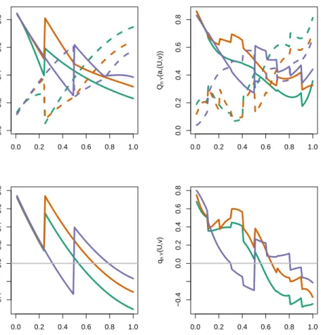
Figures 0.1 and 0.2 illustrate a typical realization. Figure 0.2 represents ¯Q0,Y, ¯q0,Y and their estimators ¯
Qn,Y, ¯qn,Y at final sample sizen= 1000. The top plot of Figure0.1 shows the 95%-CIIn in (0.9) at every sample sizenwhere a CI is derived. By Corollary0.2, the probability of the event “ψrn,0∈In” is more likely
to be close to 95% than the probability of the event “ψ0∈In” in the sense that the latter property requires that the rate of convergence of ¯qn,Y to ¯q0,Y be sufficiently fast. Nevertheless, we observe on this realization that eachIn contains both its corresponding data-adaptive parameterψrn,0 (pink cross) andψ0 (blue line).
Moreover, the difference between the length ofIn and that of the vertical segment joining the two curves of the same nuance of darker gray at sample sizengets smaller asngrows. This indicates that the variance of ψ∗n gets closer to the optimal variance VarPQ0,r0∆(Q0, r0)(O) asngrows.
The bottom plot of Figure0.1shows the actual value ofRn (green cross) and 95%-CI in (0.10) at every sample sizen where a CI is derived. We observe on this realization that the regrets are all positive, a fact that was not granted. Moreover, each CI contains its corresponding data-adaptive parameterRn.
We can evaluate if our 95%-CIs achieve their nominal 95%-coverage. To do so, we carry out binomials tests. By construction, the empirical number of CIs which cover ψrn,0 is a random variable drawn from a
Binomial distribution with parameters (N, π). We choose to test the null “π≥95%” against its one-sided alternative “π <95%”. A largep-value is interpreted as the absence of empirical evidence supporting that the CI does not achieve its nominal coverage. We do the same forψ0 andRn, mutatis mutandis.
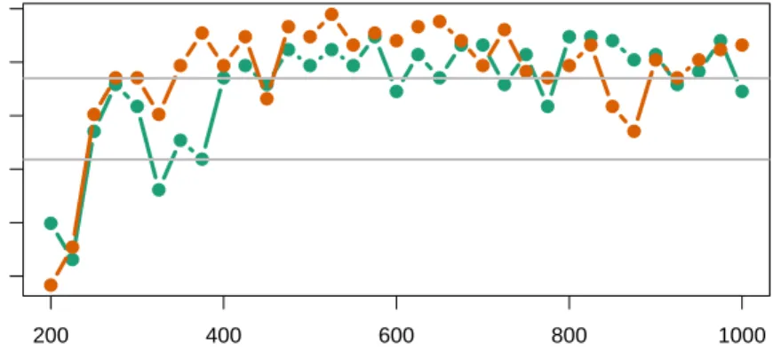
Instead of reporting 3×33 = 99 empirical proportions of coverage and relatedp-values, we simply plot the logarithms of thep-values of the tests evaluating the coverage ofψrn,0 andψ0, see Figure 0.3. Overall,
the orange curve dominates the green one, indicating that empirical coverage tends to be higher for ψrn,0
(it ranges between 0.917 and 0.955 with an average of 0.940) than forψ0 (it ranges between 0.919 and 0.946 with an average of 0.937). This does not come as a surprise, as argued in the first paragraph of this section. Moreover, a majority of thep-values are larger than 5% (top grey horizontal line), and even more of them are larger than the Bonferroni-corrected threshold of 5/33%. Furthermore, the smallestp-values correspond to sample sizesn= 200 andn= 225, where inference is based on little information. As for the coverage of Rn, it is far above the nominal 95%-coverage, ranging between 0.951 and 0.990 with an average of 0.997. This does not come as a surprise either since the CIs forRn are conservative by construction.
● ● ● ● ● ●●● ●● ● ● ● ● ● ●● ● ● ● ● ● ● ● ● ● ● ● ● ● ● ● ● 200 400 600 800 1000 0.53 0.55 0.57 0.59
Sample size at targeting steps
ψn * [0.95−confidence inter v al] Mean rewards ● ● ● ● ● ● ● ● ●● ● ● ● ● ● ● ● ● ● ● ● ● ● ● ● ● ● ● ● ● ● ● ● 200 400 600 800 1000 0.00 0.05 0.10 0.15
Sample size at updating steps
ψn *− 1 ∑ ni= 1 n Yi Regret [0.95−confidence inter v al]
Fig. 0.1. Illustrating the data-adaptive inference of the optimal rule, its mean reward and the related
regret(see also Figure0.2).Top plot.The blue horizontal line represents the value of the mean reward under the
optimal rule,ψ0. The gray curves represent the mappingn7→ψ0±ξ97.5%σk/
√
n(k= 1,2), whereσ1≈0.1512 is the
square root of VarPQ0,r0∆(Q0, r0)(O) (darker gray) and σ2 ≈0.1812 is the square root of VarPQ0,gb∆(Q0, g
b)(O)
(lighter gray). Thus, at a given sample sizen, the length of the vertical segment joining the two darker gray curves equals the length of a CI based on a regular, asymptotically efficient estimator ofψ0. The pink crosses represent the
successive values of the data-adaptive parametersψrn,0. The black dots represent the successive values ofψ
∗
n, and
the vertical segments centered at them represent the successive 95%-CIs forψrn,0and, under additional assumptions,
forψ0 as well. Bottom plot. The green crosses green represent the successive values of regret Rn. The black dots
represent the successive values ofψ∗n−n−1Pni=1Yi, and the vertical segments represent the successive 95%-CIs for
0.0 0.2 0.4 0.6 0.8 1.0 0.0 0.2 0.4 0.6 0.8 Q0 Y (a,(U ,v)) truth 0.0 0.2 0.4 0.6 0.8 1.0 −0.4 0.0 0.2 0.4 0.6 0.8 U q0 Y (U ,v) 0.0 0.2 0.4 0.6 0.8 1.0 0.0 0.2 0.4 0.6 0.8 Qn Y (a,(U ,v)) estimated 0.0 0.2 0.4 0.6 0.8 1.0 −0.4 0.0 0.2 0.4 0.6 0.8 U qn Y (U ,v)
Fig. 0.2. Illustrating the data-adaptive inference of the optimal rule, its mean reward and the related
regret through the representation of the conditional meanQ¯0,Y, blip functionq¯0,Y and their estimators
(see also Figure0.1). Top left plot.The solid curves representU 7→Q¯0,Y(1,(U, v)) for v= 1 (in dark green, lowest
value in 1),v= 2 (in dark orange, middle value in 1) andv= 3 (in dark blue, largest value in 1). The dashed curves representU7→Q¯0,Y(0,(U, v)) forv= 1 (in dark green, largest value in 1),v= 2 (in dark orange, middle value in 1)
andv= 3 (in dark blue, smallest value in 1).Bottom left plot.The curves representU 7→q¯0,Y(U, v) forv= 1 (in dark
green, smallest value in 1),v= 2 (in dark orange, middle value in 1) andv= 3 (in dark blue, largest value in 1).
Right plots. Counterparts to the left plots, where ¯Q0,Y and ¯q0,Y are replaced with ¯Qn,Y and ¯qn,Y forn= 1000, the
● ● ● ● ● ● ● ● ● ● ● ● ● ● ● ● ● ● ● ● ● ● ● ● ● ● ● ● ● ● ● ● ● 200 400 600 800 1000 −5 −4 −3 −2 −1 0
Sample size at updating steps
lo g10 (p −v alues) ● ● ● ● ● ● ● ● ● ● ● ● ● ● ● ● ● ● ● ● ● ● ● ● ● ● ● ● ● ● ● ● ●
of binomial tests on empir
ical co
v
er
age
Fig. 0.3. Empirical evaluation of the coverage of the CIs.The curves represent the logarithms ofp-values of
binomial tests of adequate coverage (null)vs.inadequate coverage (alternative). A largep-value is interpreted as the absence of empirical evidence supporting that the related CI does not achieve its nominal coverage of 95%. The dark green curve corresponds with CIs forψrn,0, and the dark orange with CIs forψ0. The gray curves show the threshold
6 Conclusion (on a twist)
We acknowledged that assuming the equality ¯q1,Y = ¯q0,Y inA1is a stringent condition. It happens that the equality is mandatory only in the context of Corollary0.1, which provides sufficient conditions for the TMLE to estimateψ0, the mean reward underr0. Yet we argued that we are more interested in the data-adaptive parameterψrn,0, the mean reward underrn, than inψ0. What can be said then without assuming ¯q1,Y = ¯q0,Y?
LetA1* be assumptionA1deprived of its condition ¯q1,Y = ¯q0,Y. In light of (0.1) and (0.5), let rule r1 and its approximationg1 be given byr1(W)≡1{¯q1,Y(W)≥0}andg1(1|W) = 1−g1(0|W)≡G(¯q1,Y(W)). Introduce
ψ1≡EQ0(Y(r1(W))),
the mean reward under ruler1. Now, letA2*be assumptionA2with7→EPQ0,g1 `( ¯Q
0
1,Y,ρ())(O)
substi-tuted for7→EPQ0,g0 `( ¯Q1,Y,ρ())(O)
, where ¯Q01,Y,ρ() is defined as in (0.6) usingg1in lieu ofg0. Introduce ¯ Q01∗,Y,r 1 ≡ ¯ Q01,Y,r 1(0(r1)) and, in light of (0.8),D 0∗ 1 given by D10∗(O)≡(Y −Q¯10∗,Y(A, W))1{A=r1(W)} g1(A|W) + ¯Q 0∗ 1,Y(r1(W), W)−ψ1, thenΣ2 1≡EPQ0,g1(D 0∗
1(O)2). Finally, consider the following counterpart toA3:
A3*. The conditional distributions ofY(0) andY(1) givenW underQ0is not degenerated. Moreover, there exist γ1, γ2>0 such that, for all t≥0,
PQ0(0≤ |¯q1,Y(W)| ≤t)≤γ1t
γ2. (0.11)
In addition, the ratio |¯q0,Y/q¯1,Y|can be defined and its (essential) supremum is finite.
The margin condition inA3* now concerns the limit blip function ¯q1,Y. The true blip function ¯q0,Y needs not take positive values Q0-almost surely anymore. As for the constraint on the ratio |¯q0,Y/q¯1,Y| (which is obviously met when ¯q1,Y = ¯q0,Y), we could simply enforce it by choosing ¯QY in such a way that|¯qY| ≥δ >0 for all ¯QY ∈Q¯Y. We may now state the final result of this manuscript.
Proposition 0.4.Under A1*, A2* and A3*, it holds that kQ¯n,Y −Q¯1,YkQ0, kq¯n,Y −q¯1,YkQ0, krn −
r1kQ0,kgn−g1kQ0 and the data-adaptive parameterψ1−ψrn,0all converge in probability to zero asntends to infinity. Furthermore, ψ∗n consistently estimates ψrn,0 hence ψ1 as well. It does so in such a way that p
n/σ2
n(ψ∗n−ψrn,0) converges in law to the standard normal distribution as n tends to infinity, where σ
2 n
consistently estimates the positiveΣ2 1.
Therefore, under the assumptions of Proposition 0.4, the CI defined in (0.9) still contains ψrn,0 with
probability tending to (1−α) as ntends to infinity. The most important result of the manuscript is thus preserved without assuming that the limit blip function and the true one coincide.
References
L. B. Balzer, M. L. Petersen, and M. J. van der Laan. Targeted estimation and inference for the sample average treatment effect. Technical Report 334, U.C. Berkeley Division of Biostatistics Working Paper Series, 2015. URLhttp://biostats.bepress.com/ucbbiostat/paper334.
B. Chakraborty and E. E. M. Moodie. Statistical methods for dynamic treatment regimes. Statistics for Biology and Health. Springer, New York, 2013. doi: 10.1007/978-1-4614-7428-9. URLhttp://dx.doi. org/10.1007/978-1-4614-7428-9. Reinforcement learning, causal inference, and personalized medicine. B. Chakraborty, E. B. Laber, and Y-Q. Zhao. Inference about the expected performance of a data-driven
dynamic treatment regime. Clin. Trials, 11(4):408–417, 2014.
A. Chambaz and M. J. van der Laan. Inference in targeted group-sequential covariate-adjusted randomized clinical trials. Scand. J. Stat., 41(1):104–140, 2014. doi: 10.1111/sjos.12013. URLhttp://dx.doi.org/ 10.1111/sjos.12013.
A. Chambaz, M. J. van der Laan, and W. Zheng. Targeted covariate-adjusted response-adaptive lasso-based randomized controlled trials. In A. Sverdlov, editor, Modern Adaptive Randomized Clinical Trials: Statistical, Operational, and Regulatory Aspects, pages 345–368. CRC Press, 2015.
A. Chambaz, W. Zheng, and M. J. van der Laan. Data-adaptive inference of the optimal treatment rule and its mean reward. The masked bandit. Technical report, 2016. URL https://hal.archives-ouvertes. fr/hal-01301297.
V. H. de la Pe˜na and E. Gin´e.Decoupling. Probability and its Applications (New York). Springer-Verlag, New York, 1999. doi: 10.1007/978-1-4612-0537-1. URL http://dx.doi.org/10.1007/978-1-4612-0537-1. From dependence to independence, Randomly stopped processes.U-statistics and processes. Martingales and beyond.
J. Friedman, T. Hastie, and R. Tibshirani. Regularization paths for generalized linear models via coordinate descent. Journal of Statistical Software, 33(1):1–22, 2010. URLhttp://www.jstatsoft.org/v33/i01/. Y. Goldberg, R. Song, D. Zeng, and M. R. Kosorok. Comment on “Dynamic treatment regimes: Technical
challenges and applications”. Electron. J. Stat., 8:1290–1300, 2014.
E. B. Laber, D. J. Lizotte, M. Qian, W. E. Pelham, and S. A. Murphy. Dynamic treatment regimes: Technical challenges and applications. Electron. J. Stat., 8(1):1225–1272, 2014a.
E. B. Laber, D. J. Lizotte, M. Qian, W. E. Pelham, and S. A. Murphy. Rejoinder of “Dynamic treatment regimes: Technical challenges and applications”. Electron. J. Stat., 8(1):1312–1321, 2014b.
A. R. Luedtke and M. J. van der Laan. Targeted learning of the mean outcome under an optimal dynamic treatment rule. Journal of Causal Inference, 3(1):61–95, 2015a.
A. R. Luedtke and M. J. van der Laan. Statistical inference for the mean outcome under a possibly non-unique optimal treatment strategy. Ann. Statist., 2015b. To appear.
A. R. Luedtke and M. J. van der Laan. Super-learning of an optimal dynamic treatment rule. International Journal of Biostatistics, 2016. To appear.
E. Mammen and A. B. Tsybakov. Smooth discrimination analysis. Ann. Statist., 27(6):1808–1829, 1999. doi: 10.1214/aos/1017939240. URLhttp://dx.doi.org/10.1214/aos/1017939240.
J. Pearl. Causality: Models, Reasoning and Inference, volume 29. Cambridge University Press, Cambridge, 2000.
M. Qian and S. A. Murphy. Performance guarantees for individualized treatment rules. Ann. Statist., 39(2): 1180–1210, 2011. doi: 10.1214/10-AOS864. URLhttp://dx.doi.org/10.1214/10-AOS864.
J. M. Robins. Optimal structural nested models for optimal sequential decisions. In D. Y. Lin and P. Heagerty, editors,Proc. Second Seattle Symp. Biostat., pages 189–326, 2004.
D. B. Rubin and M. J. van der Laan. Statistical issues and limitations in personalized medicine research with clinical trials. Int. J. Biostat., 8(1), 2012. Article 1.
A. W. van der Vaart and J. A. Wellner. Weak Convergence. Springer, 1996.
B. Zhang, A. Tsiatis, M. Davidian, M. Zhang, and E. Laber. A robust method for estimating optimal treatment regimes. Biometrics, 68:1010–1018, 2012a.
B. Zhang, A. Tsiatis, M. Davidian, M. Zhang, and E. Laber. Estimating optimal treatment regimes from a classification perspective. Stat, 68(1):103–114, 2012b.
Y. Zhao, D. Zeng, A. J. Rush, and M. R. Kosorok. Estimating individualized treatment rules using outcome weighted learning.J. Amer. Statist. Assoc., 107(499):1106–1118, 2012. doi: 10.1080/01621459.2012.695674. URLhttp://dx.doi.org/10.1080/01621459.2012.695674.
Y. Zhao, D. Zeng, E. B. Laber, and M. R. Kosorok. New statistical learning methods for estimating optimal dynamic treatment regimes. J. Amer. Statist. Assoc., 110(510):583–598, 2015. doi: 10.1080/01621459. 2014.937488. URLhttp://dx.doi.org/10.1080/01621459.2014.937488.
W. Zheng, A. Chambaz, and M. J. van der Laan. Drawing valid targeted inference when covariate-adjusted response-adaptive rct meets data-adaptive loss-based estimation, with an application to the LASSO. Technical Report 339, U.C. Berkeley Division of Biostatistics Working Paper Series, 2015. URL