A regression tree approach using mathematical programming

(1)

Contents lists available at ScienceDirect

Expert

Systems

With

Applications

journal homepage: www.elsevier.com/locate/eswa

A

regression

tree

approach

using

mathematical

programming

Lingjian

Yang

a

_,

_Songsong

_Liu

a , b

_,

_Sophia

_Tsoka

c

_,

_Lazaros

_G.

_Papageorgiou

a , ∗

a_Centre_for_Process_Systems_Engineerig,_Department_of_Chemical_Engineering,_University_College_London,_Torrington_Place,_London_WC1E_7JE,_UK b_School_of_Management,_Swansea_University,_Bay_Campus,_Fabian_Way,_Swansea_SA1_8EN,_UK

c_Department_of_Informatics,_King’s_College_London,_Strand,_London_WC2R_2LS,_UK

a

r

t

i

c

l

e

i

n

f

o

Articlehistory:

Received13July2016 Revised4February2017 Accepted5February2017 Availableonline9February2017

Keywords: Regressionanalysis Surrogatemodel Regressiontree Mathematicalprogramming Optimisation

a

b

s

t

r

a

c

t

Regressionanalysisisamachinelearningapproachthataimstoaccuratelypredictthevalueof contin-uousoutputvariablesfromcertainindependentinputvariables,viaautomaticestimationoftheirlatent relationshipfromdata.Tree-basedregressionmodelsarepopularinliteratureduetotheirflexibilityto model higherordernon-linearity and greatinterpretability. Conventionally, regressiontreemodelsare trainedinatwo-stageprocedure,i.e.recursivebinarypartitioningisemployedtoproduce atree struc-ture,followed byapruning process ofremoving insignificant leaves,withthe possibility ofassigning multivariatefunctionstoterminalleavestoimprovegeneralisation.Thisworkintroducesanovel method-ologyofnodepartitioningwhich,inasingleoptimisationmodel,simultaneouslyperformsthetwotasks ofidentifyingthebreak-pointofabinarysplitandassignmentofmultivariatefunctionstoeither leaf, thusleadingtoanefficientregressiontreemodel.Usingsixrealworldbenchmarkproblems,we demon-stratethatthe proposedmethodconsistentlyoutperformsanumberofstate-of-the-artregressiontree modelsandmethods basedonothertechniques, withanaverageimprovement of7–60%onthemean absoluteerrors(MAE)ofthepredictions.

1. Introduction

In machine learning, regression analysis seeks to estimate the relationships between output variables and a set of independent input variables by automatically learning from a number of cu- rated samples ( Sen & Srivastava, 2012 ). The primary goal of applying a regression analysis is usually to obtain precise prediction of the level of output variables for new samples. Examples of methodologies for regression analysis in the literature include linear regression ( Seber & Lee, 2012 ), automated learning of algebraic models for optimisation (ALAMO) ( Cozad, Sahinidis, & Miller, 2014; Zhang & Sahinidis, 2013 ), support vector regression (SVR) ( Smola & Schlkopf, 2004 ), multilayer perception (MLP) ( Hill, Marquez, O’Connor, & Remus, 1994 ), K-nearest neighbour (KNN) ( Korhonen & Kangas, 1997 ), multivariate adaptive regression splines (MARS) ( Friedman, 1991 ), Kriging ( Kleijnen, 2015 ), and regression tree.

Quite often, one would like to also gain some useful insights into the underlying relationship between the input and output variables, in which case the interpretability of a regression method

∗ _{Corresponding}_author.

E-mailaddresses:[email protected](L.Yang),

[email protected](S.Liu),[email protected](S.Tsoka),

[email protected](L.G.Papageorgiou).

is also of great interest. Regression tree is a type of the machine learning tools that can satisfy both good prediction accuracy and easy interpretation, and therefore have received extensive attention in the literature. Regression tree uses a tree-like graph or model and is built through an iterative process that splits each node into child nodes by certain rules, unless it is a terminal node that the samples fall into. A regression model is ﬁtted to each terminal node to get the predicted values of the output variables of new samples.

The Classification and Regression Tree (CART) is probably the most well known decision tree learning algorithm in the literature ( Breiman, Friedman, Olshen, & Stone, 1984 ). Given a set of samples, CART identifies one input variable and one break-point, before partitioning the samples into two child nodes. Starting from the entire set of available training samples (root node), recursive binary partition is performed for each node until no further split is possible or a certain terminating criteria is satisfied. At each node, best split is identified by exhaustive search, i.e. all potential splits on each input variable and each break-point are tested, and the one corresponding to the minimum deviations by respectively predicting two child nodes of samples with their mean output variables is selected. After the tree growing procedure, typically an overly large tree is constructed, resulting in lack of model generalisation to unseen samples. A procedure of pruning is employed to remove http://dx.doi.org/10.1016/j.eswa.2017.02.013

(2)

sequentially the splits contributing insufficiently to training accuracy. The tree is pruned from the maximal-sized tree all the way back to the root node, resulting in a sequence of candidate trees. Each candidate tree is tested on an independent validation sample set and the one corresponding to the lowest prediction error is selected as the final tree ( Breiman, 20 01; Wu et al., 20 08 ). Alter- natively, the optimal tree structure can be identified via cross validation. After building a tree, an enquiry sample is firstly assigned into one of the terminal leaves (non-splitting leaf nodes) and then predicted with the mean output value of the samples belonging to the leaf node. Despite its simplicity, good interpretation and wide applications ( Antipov & Pokryshevskaya, 2012; Bayam, Liebowitz, & Agresti, 2005; Bel, Allard, Laurent, Cheddadi, & Bar-Hen, 2009; Li, Sun, & Wu, 2010; Molinaro, Dudoit, & van der Laan, 2004 ), the simple rule of predicting with mean values at the terminal leaves often means prediction performance is compromised ( Loh, 2011 ).

The conditional inference tree (ctree) tackles the problem of recursive partitioning in a statistical framework ( Hothorn, Hornik, & Zeileis, 2006 ). For each node, the association between each independent input feature and the output variable is quantiﬁed, using permutation test and multiple testing correction. If the strongest association passes a statistical threshold, binary split is performed in that corresponding input variable; otherwise the current node is a terminal node. Ctree is shown to avoid the problem of building biased tree towards input variables with many distinct levels of values while ensuring the similar prediction performance.

Since almost all the tree-based learning models are constructed using recursive partitioning, an efficient yet essentially locally optimal approach, the evtree implements an evolutionary algorithm for learning globally optimal classification and regression trees ( Grubinger, Zeileis, & Pfeiffer, 2014 ), and is considered an alterna- tive to the conventional methods by globally optimising the tree construction. Evtree searches a tree structure that takes into account the accuracy and complexity, defined as the number of terminal leaves. Due to the exponentially growing size of the problem, evolutionary methods are employed to identify a quality fea- sible solution.

M5’, also knows as M5P, is considered as an improved version of CART ( Quinlan, 1992; Wang & Witten, 1997 ). The tree growing process is the same as that of the CART, while several modifica- tions have been introduced in tree pruning process. After the full size tree is produced, a multiple linear regression model is fitted for each node. A metric of model generalisation is defined in the original paper taking into account training error, the numbers of samples and model parameters. The constructed linear regression function for each node is then simplified by removing insignificant input variables using a greedy algorithm in order to achieve locally maximal model generalisation metric. Tree pruning starts from the bottom of the tree and is implemented for each non-leaf nodes. If the parent node offers higher model generalisation than the sum of the two child nodes, then the child nodes are pruned away. When predicting new samples, the value computed at the corresponding terminal node is adjusted by taking into account the other predicted values at the intermediate nodes along the path from the terminal to the root node. The fitting of linear regression functions at leaf nodes improves the prediction accuracy of the regression tree learning model.

M5’ is then further extended into Cubist ( RuleQuest, 2016 ), a commercially available rule-based regression model, which has received increasing popularity recently ( Kobayashi, Tsend-Ayush, & Tateishi, 2013; Minasny & McBratney, 2008; Moisen et al., 2006; Peng et al., 2015; Rossel & Webster, 2012 ). M5’ is employed to grow a tree ﬁrst, which is then collapsed into a smaller set of if-then rules by removing and combining paths from the root to the terminal nodes. It is noted here that the if-then rules resulted from Cubist method can be overlapping, i.e. a sample can be assigned

into multiple rules, where all the predictions are averaged to pro- duce a ﬁnal value. This ambiguity decreases the interpretability of the rule model.

The Smoothed and Unsmoothed Piecewise-Polynomial Regres- sion Trees (SUPPORT) is another regression tree learning algorithm, whose foundation is based on statistics ( Chaudhuri, Huang, Loh, & Yao, 1994 ). Given a set of samples, SUPPORT ﬁts a multiple linear regression function and computes the deviation of each sample. The samples with positive deviations and negative deviations are respectively assigned into two classes. For each input variable, SUPPORT compares the distribution of the two classes of samples along this input variable by applying two-sample t test. The input variable corresponding to the lowest P value is selected as splitting node and the average of the two class mean on this splitting variable is taken as break-point.

The Generalised, Unbiased, Interaction Detection and Estimation (GUIDE) adopts similar philosophy as the SUPPORT ( Loh, 2002; Loh, He, & Man, 2015 ). Given a node, the same step of fitting samples with a linear regression model and separating samples into two classes based on the sign of deviations is employed. For each input variable, its numeric values are binned into a number of in- tervals before a chi-square test is used to determine its level of significance. The most significant input variable is used for binary split. In terms of break-point determination, either a greedy search or median of the two class mean on this splitting variable can be used.

More other variants of the above regression tree models also exist in the literature, including SECRET ( Dobra & Gehrke, 2002 ), MART ( Elish, 20 09; Friedman, 20 02 ), SMOTI ( Malerbao, Espos- ito, Ceci, & Appice, 2004 ), MAUVE ( Vens & Blockeel, 2006 ), BART ( Chipman, George, & McCulloch, 2010 ) and SERT ( Chen & Hong, 2010 ), etc.

In the above classic regression tree methodologies, the tradi- tional means of node splitting are dominated by either exhaus- tively searching the candidate split corresponding to the maximum variance reduction by predicting of mean output values in two child nodes ( Breiman et al., 1984; Quinlan, 1992; Wang & Witten, 1997 ), or examining distribution of sample deviations from fitting one linear regression function to all the samples in the parent node ( Chaudhuri et al., 1994; Loh, 2002 ). However, it is noticed that for those algorithms where terminal leaf nodes are fitted with linear regression functions ( Quinlan, 1992; Wang & Witten, 1997 ), the choice of splitting variable, break-point and regression coefficients are done sequentially, i.e. the splitting variable and break-point are estimated during tree growing procedure while regression coefficients for each child node are computed at pruning step.

A theoretically better node splitting strategy is to simultaneously determine the splitting feature, the position of break-point and the regression coefficients for each child node. In this case, the quality of a split can be directly calculated as the sum of deviations of all samples in either subset. A straightforward exhaustive search algorithm for this problem can be: for each input variable and each break-point, samples are separated into two subsets and one multiple linear regression is fitted for each subset. After examining all possible splits, the optimal split is chosen as the one corresponding to the minimum sum of deviations. The problem with this approach is, however, that as the numbers of samples and input variables grow, the quantity of multiple linear regression functions need to be evaluated increases exponentially, re- quiring excessive computational time. For example, given a regression problem of 500 samples and 10 input variables, we assume for each input variable, each sample takes a unique value. Then it requires construction of 9980 ( =499 × 10 × 2) multiple linear regression functions in order to find the optimal split for only the root node, which will only become worse as the tree grows larger.

(3)

In this work, we adopt a recently proposed mathematical programming optimisation model ( Yang, Liu, Tsoka, & Papageorgiou, 2016 ), which solves the problem of splitting a node into two child nodes to global optimality in affordable computational time. In our proposed framework, tree leaf nodes are ﬁtted with polynomial functions and recursive partition is permitted when the amount of reduction in deviation achieved by node splitting is above a user-speciﬁc value, which is also the only tuning parameter in our framework. Since the size of the tree is controlled via the tuning parameter, the pruning procedure is not implemented.

The rest of the paper is structured as follows: In Section 2 , we describe the main features of the optimisation model adopted from literature and introduces the framework of our proposed decision tree building process. In Section 3 , a number of benchmark regression problems are employed to test the performance of our proposed method. A comprehensive sensitivity analysis is con- ducted to evaluate how prediction accuracy varies with different values of the tuning parameter. Later, prediction accuracy of our proposed method is compared against a number of decision tree based algorithms and some other state-of-the-art regression methods. Section 4 presents our main conclusions and discusses some future directions.

2. Method

In our previous work ( Yang et al., 2016 ), we have proposed a regression method based on piece-wise linear functions, named segmented regression. Segmented regression identifies multiple break- points on a single independent variable and partitions the samples into multiple regions, each one of which is fitted with a multiple linear regression function so as to minimise the absolute deviation of the samples. The core element of the segmented regression is a mathematical programming optimisation model that, given one single input variable as splitting variable and the number of regions, simultaneously optimises the positions of the break-points and the regression coefficients of one multiple linear regression function for each region.

In this work, we adopt this optimisation model to optimise binary splitting of nodes. Given a node and a single input variable as splitting variable, the optimisation model is solved to find the single break-point and the regression coefficients for the two child nodes. The model is solved when each input variable in turn serves as splitting variable once, and the input variable giving the minimum absolute deviation is selected for splitting the current parent node. Recursive node splitting terminates when the reduction in deviation drops below a user-specific threshold value. Below, the overview of the regression approach, and the detailed mathematical programming model for node partitioning are presented. 2.1. Regressiontreeapproach

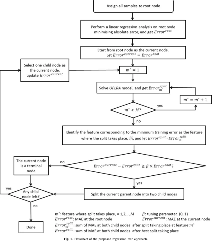
As for other regression tree learning algorithms, recursive splitting is used to grow the tree from root node until a split of node cannot yield suﬃcient reduction in deviation. The pseudocode for building a tree is given below.

Proposed regression tree algorithm

Step1. Fitapolynomialregressionfunctionoforder2torootnode minimisingabsolutedeviation,recordedasERRORroot_. Step2. Startfromtherootnodeasthecurrentnode,andlet

ERRORcurrent₌_E_RRORroot_.

Step3. Ineachcurrentroot,foreachinputvariablem,specifyitassplitting variable(m=m∗₎_and_solve_the_proposed_Optimal_Piece-wise_Linear

RegressionAnalysismodel(OPLRA).Thedeviationisnotedas

ERRORsplit m .

Step4. Identifythebestsplitcorrespondingtotheminimumabsolute deviation,notedasERRORsplit₌_min

m ERROR split m .

Step5. IfERRORcurrent₋_E_RRORsplit_≥_β_×_E_RRORroot_,_the_current_node_is_split;

otherwisethecurrentnodeisﬁnishedasaterminalnode.

Step6. Applystep3–5toeachremainingchildnodeinturn.

Given training samples, the ﬁrst step of our proposed tree growing strategy is to ﬁt a polynomial regression function of order of 2 to the entire set of training samples minimising absolute deviation, which is noted as ERRORroot_{. The}_{used polynomial}_re-

gression function can provide higher prediction accuracy. Note that when the coeﬃcient of the quadratic term is zero, the obtained regression model is a linear function. The absolute deviation is min- imised here, due to its simplicity and ease of optimisation. The absolute deviation of root node, multiplied by a scaling parameter

β

, taking value between 0 and 1, is speciﬁed as the condition for node splitting. In other words, the current node is split into two child nodes, only if the optimal split of the node results in reduction of absolute deviation being greater than

β

×ERRORroot_{. Then starting}

from the root node as the current node, each feature m is speciﬁed in turn as splitting feature m∗ once, while solving model OPLRA minimising the sum of absolute deviations of two child nodes. The best split of the current node is identiﬁed as the one corresponding to minimum absolute error. If the best split brings down absolute deviation from the current node ( ERRORcurrent_{) by more than}

β

× ERRORroot_{, then the split takes place; otherwise the current}

node is ﬁnalised as terminal leaf node. Note that the tuning parameter

β

determines the size of the developed tree, and an ap- propriate value of

β

can avoid the overﬁtting on the training data, and achieve good prediction accuracy for testing. The ﬂowchart of the whole procedure is illustrated in Fig. 1 .

2.2.Mathematicalprogrammingmodelfornodepartitioning

For a given current node n and one feature m*_{for potential par-} tition, the proposed mathematical programming model for the optimal node split, OPLRA, is presented in this section. The indices, sets, parameters and variables associated with the model are listed below. For better separation between the parameters and variables, here lower case letters are for parameters, while upper case letters are for variables:

Indices

c childnodeofthecurrentparentnoden;c₌l representsleft childnode,andc=rrepresentsrightchildnode

m feature/independentinputvariable,m= 1 ,2 ,...,M m∗ thefeaturewheresamplepartitiontakesplace n thecurrentparentnode

s samplesinthedataset,s=1 ,2 ,...,S Sets

Cn setofchildnodesofthecurrentparentnoden Sn setofsamplesinthecurrentparentnoden

Parameters

asm numericvalueofsamplesonfeaturem ys realoutputvalueofsamples

u asuitablylargepositivenumber

asuitablysmallpositivenumber Continuous variables

Bc _intercept_of_regression_function_in_child_node_c Ds absolute deviation between predicted output and real

outputforsamples Pc

s predictedoutputforsamplesinchildnodec W1 c

m,W2 cm regressioncoeﬃcientsforfeatureminchildnodec Xm∗ break-pointonpartitionfeaturem∗

(4)

Fig. 1. Flowchartoftheproposedregressiontreeapproach.

Binary variables Fc

s 1ifsamplesfallsintochildnodec;0otherwise

Binary variables Fc

s, taking value of either 0 or 1, are introduced

to model if sample s belongs to child node c or not. Modelling of which sample belongs to either child node is achieved with the following constraints:

asm∗≤X_m∗−

+u

(

1−F_sc

)

∀

s∈S_n,c=l,m∗ (1) Xm∗+

−u

(

1−F_sc

)

≤a_sm∗

∀

s∈S_n,c=r,m∗ (2)

When sample s is assigned into left child node (i.e. Fc

s = 1 when c=l), Eq. (1) becomes Asm∗≤Xm∗−

while Eq. (2) becomes re-

dundant. On the other hand, when sample s is assigned into right

child node (i.e. Fc

s =1 when c=r), Eq. (2) becomes Asm∗≥Xm∗+

while Eq. (1) is redundant. The insertion of

is to ensure strict separation of the samples into two child nodes. The following constraints restrict that each sample belongs to one and only one child node:

c∈Cn Fc

s =1

∀

s∈Sn (3)

For each child node c, polynomial functions of order 2 is employed to predict the value of samples ( Pc

s): Psc= m a2smW2cm+ m asmW1cm+Br

∀

s∈Sn,c∈Cn (4)

For any sample s, its training error is equal to the absolute deviation between the real output and the predicted output for the

(5)

child node c where it belongs to (i.e. Fc

s =1 ), and can be expressed

with the following two equations:

Ds≥ys−Psc−u

(

1−Fsc

)

∀

s∈Sn,c∈Cn (5)

Ds≥Psc−ys−u

(

1−Fsc

)

∀

s∈Sn,c∈Cn (6)

The objective function is to minimise the sum of absolute training errors of splitting the currentnoden into its child nodes:

min s∈Sn

Ds (7)

The ﬁnal OPLRA model consists of a linear objective function and several linear constraints, and the presence of both binary and continuous variables deﬁne an MILP problem, which can be solved to global optimality by standard solution algorithms, for example branch and bound. The optimisation model simultaneously optimises the break-point ( Xm∗), the allocation of samples into two

child nodes ( Fc

s) and the regression coeﬃcients ( W1 cm,W2 cm and Bc_{) to achieve the least absolute deviation. Another advantage of}

this optimisation model is that there is no need to pre-process input variable, i.e. input variables do not need to be binned into in- tervals for analysis.

2.3. Predictionfornewsamples

After the regression tree is determined, prediction of new enquiry samples can easily be performed. A new sample is ﬁrstly assigned to one of the terminal leaf node, before yielding a prediction using the multivariate function derived for that particular node. The predicted output value, if lies outside the interval bounded by the minimum and maximum of ﬁtted output values for training samples in that particular node, is then adjusted to the nearest bound.

The proposed regression tree approach, referred to as Mathe- matical Programming Tree (MPTree) in this paper, is applied to a number of real world benchmark data sets in the next section to demonstrate its applicability and eﬃciency.

3. Resultsanddiscussion

In this section, we aim to comprehensively evaluate the be- haviour of the proposed MPTree using real world benchmark data sets. We ﬁrst conduct a comprehensive sensitivity analysis for the tuning parameter

β

in order to identify a robust value that gives consistently good prediction accuracy. After that, prediction accuracy comparison is performed to evaluate MPTree against certain popular regression tree learning algorithms in literature and some other regression methodologies.

A total number of 6 real world regression data sets have been downloaded from UCI machine learning repository ( Lichman, 2013 ). The first regression problem Yacht Hydrodynamics predicts the residuary resistance of sailing yachts at the initial design stage from 6 independent features describing the hull dimensions and velocity of the boat, including longitudinal position of the centre of buoyancy, prismatic coefficient, length-displacement ratio, beam-draught ratio, length-beam ratio and Froude number. The next example, Concrete Strength ( Yeh, 1998 ), studies how com- pressive strength of different concrete are affected by attributes of the concretes. There are 1030 samples with 8 input attributes, such as cement, blast furnace slag, fly ash, water, superplasticizer, coarse aggregate, fine aggregate and age. Energy Efficiency data sets ( Tsanas & Xifara, 2012 ) are obtained by running simulation model. There are 768 samples, with each corresponding to one building shape, described by 8 features including relative compact- ness, surface area, wall area, root area, overall height, orientation,

Table 1

Summaryofbenchmarkdatasets.

Casestudy Numberofsamples Numberoffeatures Yachthydrodynamics 308 6

Concretestrength 1030 8 Energyeﬃciencyheating 768 8 Energyeﬃciencycooling 768 8

Airfoil 1503 5

Whitewinequality 4898 11

glazing area and glazing area distribution. The aims are to establish the relationship between either heating or cooling load require- ment of the building and the characteristics of these building. Air- foil data set concerns how the different frequencies, chord lengths, angles of attack, free-stream velocities and suction side displacement thicknesses can predict the sound pressure level of an airfoil. The last case study, White Wine Quality ( Cortez, Cerdeira, Almeida, Matos, & Reis, 2009 ), aims to associate expert preference of white wine taste with 11 physicochemical features of the wines, including ﬁxed acidity, volatile acidity, citric acid, residual sugar, chlorides, free sulfur dioxide, total sulfur dioxide, density, pH, sul- phates and alcohol. The details of these data sets are provided as the supplementary material, and their sizes are summarised in Table 1 .

For each regression problem, we employ a 5-fold cross validation to estimate the predictive accuracy of various regression methods. Given a data set, 5-fold cross validation randomly splits the samples into 5 subsets of roughly equal size. One subset is hold out as testing set, while the other 4 subsets of samples are merged to form training set. MPTree constructs a regression tree on the training set, whose prediction accuracy is estimated using the holdout testing set. The process continues until each subset is hold out once as testing set. We conduct 10 rounds of 5- fold cross validation by performing different random sample splits, and the mean absolute errors (MAE) of the prediction are averaged over 50 testing sets as the ﬁnal error. For each data set, we normalise each independent input variable with the following formula so that the scaled input data take value between 0 and 1: Asm= A

sm−minsAsm

maxsA_sm−minsA_sm

∀

s,m, where Asmdenotes the raw input

data.

To assess the relative competitiveness of the proposed MPTree in terms of prediction accuracy, we compare the proposed MPTree to a number of popular regression methods in literature, including CART, M5’, Cubist, linear regression, SVR, MLP, Kriging, KNN, MARS, segmented regression ( Yang et al., 2016 ) and ALAMO. CART, ctree, evtree and Cubist are implemented in R ( R Development Core Team, 2008 ) using the packages ‘rpart’, ‘party’, ‘evtree’ and ‘Cubist’, respectively. M5’, linear regression, SVR, MLP, kriging and KNN are implemented in WEKA machine learning software ( Hall et al., 2009 ). For KNN, the number of nearest neighbours is selected as 5, while for other methods their default settings have been retained. We use the MATLAB toolbox called ARESlab for MARS. ALAMO is reproduced using the General Algebraic Model- ing System (GAMS) ( GAMS Development Corporation, 2014 ), and basis function forms including polynomial of degrees up to 3, pair- wise multinomial terms of equal exponents up to 3, exponen- tial and logarithmic forms are provided for each data set. Seg- mented regression and the proposed MPTree are also implemented in GAMS. ALAMO, segmented regression and our proposed MPTree are solved using CPLEX MILP solver, with optimality gap set as 0. All computational runs were performed on a 64-bit Windows 7 based machine with 3.20 GHz six-core Intel Xeon processor W3670 and 12.0 GB RAM.

(6)

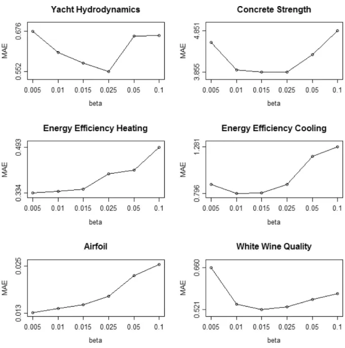
Fig. 2. Sensitivityanalysisforβofalldatasets.

3.1.Sensitivityanalysisfor

β

In this section, we ﬁrst perform a comprehensive sensitivity analysis on the single tuning parameter

β

in the proposed MPTree. Recall in the tree growing procedure,

β

controls termination of recursive node splitting. A node is split into two child nodes if the optimal split leads to reduction of absolute training deviation being more than a threshold value, deﬁned as the amount of absolute training deviation of a multiple linear regression analysis on the entire set of training samples ERRORrootmultiplied by the scal-

ing parameter

β

. The tree grows larger as

β

decreases. Identifying a suitable value for

β

is a non-trivial problem as an excessively high value would terminate the node splitting prematurely with- out adequately describing the data, while a very small value can over-ﬁt the unseen samples by constructing very large trees. In this work, we test a series of values, including 0.005,0.01,0.015,0.025, 0.05 and 0.1. The results of the sensitivity analysis are presented in Fig. 2 .

According to Fig. 2 , we can clearly observe a phenomenon that as

β

is reduced from 0.1 to 0.015, prediction error almost mono-

tonically drops. This improved prediction performance can be at- tributed to the fact that decreased

β

allows the tree to grow larger, and thus better describing the latent pattern in the data. As

β

further lowers down, MAE can even further decreases for some examples, including Energy Eﬃciency Heating and Airfoil. For some other examples, including Yacht Hydrodynamics, Concrete Strength, Energy Eﬃciency Cooling and White Wine Quality, more complicating trees do not predict unseen testing samples well, as MAE worsens.

It is well known that in data mining, parameter ﬁne tuning is required for a particular method to reach optimal performance for a speciﬁc data set. Thus, it is our interest here to identify a value for

β

that corresponds to robust prediction accuracy for a range of different tested benchmark examples. In this study,

β

= 0.015 appears to yield overall robust and accurate prediction as it usually leads to lowest or second lowest MAE among all the tested values. Higher values of

β

are shown to give signiﬁcantly higher MAE, while smaller value of

β

sometimes leads to noticeable over- ﬁtting, thus compromising the robustness of its performance.

(7)

Table 2

Predictionaccuracycomparisonacrossdifferentregressionmethods,intermsofMAE.TheproposedMPTreemethodis high-lightedinitalic,andthebestpredictionaccuracyofeachdatasetisgiveninbold.

Yacht Concrete Energyeﬃciency Energyeﬃciency Airfoil Whitewine hydrodynamics strength heating cooling quality Tree-basedmethods MPTree 0.58 3.85 0.35 0.80 0.015 0.52 CART 1.61 7.22 2.00 2.38 0.035 0.60 Ctree 0.81 5.99 0.63 1.40 0.029 0.58 Evtree 1.05 6.44 0.56 1.59 0.032 0.59 M5’ 0.96 4.72 0.69 1.21 0.021 0.56 Cubist 0.60 4.29 0 .35 0.89 0.017 0.56 Non-tree-basedmethods Linearregression 7.27 8.31 2.09 2.27 0.037 0.59 SVR 6.45 8.21 2.04 2.19 0.037 0.58 MLP 0.81 6.23 0.99 1.92 0.035 0.62 Kriging 4.32 6.22 1.79 2.04 0.030 0.58 KNN 5.30 7.07 1.94 2.15 0.026 0.54 MARS 1.01 4.87 0.80 1.32 0.035 0.57 Segmentedregression 0.71 4.87 0.81 1.28 0.029 0.55 ALAMO 0.79 8.04 2.72 2.76 0.032 0.64

Fig. 3. Predictionaccuracy (MAE)comparison acrossdifferent regression methods.Foreach benchmarkexample,the originalMAEachieved bydifferentmethodsin

Table2arenormalisedbetween0%and100%,with0%representingthelowestMAEand100%representingthehighestMAE.

3.2. Performancecomparisonacrossdifferentregressionmethods After identifying a value (i.e. 0.015) for the only user-speciﬁc parameter,

β

, in the proposed MPTree, we now compare the prediction performance of the MPTree against a number of state-of-the- art regression methods. To ensure unbiased comparison,

β

is set to 0.015 thorough all examples studied. For each of the benchmark examples, we compare the MAE achieved by various competing methods. The detailed prediction accuracies reported in Table 2 , in which the performance of the proposed MPTree method is shown in italic, and the best prediction accuracy, i.e. the smallest MAE, of each data set is given in bold. The proposed has the best prediction accuracy in all data sets, compared to regression methods based on a wide range of tree and non-tree methodologies. Only in the Energy Eﬃciency Heating data set, Cubist achieves the same

accuracy as MPTree. Overall, MPTree achieves 7–60% of improvement on MAE compared to each of other regression models. We have also implemented MPTree with linear function at each child node, the results of which still show great competitiveness as being either the top or the second best method in all examples and achieves the overall best performance with MAE values of 0.60, 4.16, 0.36, 1.00, 0.014 and 0.55, respectively.

The comparative results are summarised in Fig. 3 . This Radar chart is plotted to comprehensively visualise the prediction performance of different methods across all 6 data sets. For each benchmark example studied, we normalise the MAE achieved by all methods in Table 2 to scaled values between 0% and 100%, with 0% and 100% respectively denoting the lowest and the highest MAE. To maintain the readability of the plot, prediction accuracies of only 7 methods are plotted. It is clearly observed from Fig. 3 that the

(8)

Table 3

Predictionaccuracycomparisonacrossdifferenttree-basedregressionmethodsintermsofMSE.Theproposed MPTreemethodishighlightedinitalic,andthebestpredictionaccuracyofeachdatasetisgiveninbold.

Yacht Concrete Energyeﬃciency Energyeﬃciency Airfoil Whitewine hydrodynamics strength heating cooling quality

MPTree 2.03 43.88 0.26 2.65 0.0005 0.59 CART 5.41 86.24 6.85 9.40 0.0020 0.58 Ctree 2.79 63.72 1.33 4.37 0.0014 0.55 Evtree 3.02 69.12 1.00 4.44 0.0015 0.56 M5’ 3.08 40.72 0.95 3.26 0.0008 0.53 Cubist 1 .07 37 .77 0.27 2.76 0.0006 0 .51

Fig. 4. ConstructedtreebyCARTonEnergyEﬃciencyHeatingexample.Boxesrepresenttheterminalleafnodeswithlabelsinside,whilecirclesrepresentothernodes, wherethesymbolinsidereferstothefeaturewherethesplittakesplace.Thesplittingrulesaregivenonthecorrespondingpaths.

proposed MPTree forms the smallest area across all data sets, and performs better than other implemented tree-based learning algorithms, including ctree, evtree, M5’ and Cubist, and non-tree-based models, including MLP and Segmented regression. Overall, MPTree demonstrates clear advantage over the counterparts by managing the lowest MAE value for each and every tested benchmark example (including SVR, Kriging and KNN where results are not shown here). It is undoubtedly that the proposed MPTree, by optimising simultaneously the position of break-point and regression coeﬃ- cients per child node, representing signiﬁcant improvement compared with other tree models in literature.

In this work, MAE is adopted as the performance metric of regression models, which might not be suitable for all the data sets. Besides, other approaches might provide better ﬁttings over another performance metric, e.g., mean squared error (MSE), root mean squared error (RMSE), Akaike Information Criterion, etc. When we compare the prediction accuracy in terms of MSE of all tree-based methodologies, Table 3 shows that the post-processed

MSE values from the optimal solutions of MPTree are still very competitive with MSE values from other methodologies, even the proposed MPTree aims to minimise MAE. Although the performance of MPTree is not as dominant as it is considering MAE, MPTree still ranks ﬁrst on three data sets out of six, and is comparable with Cubist, which performs the best for the other three data sets. These results demonstrate the impact of performance metrics on the predication performance, and the consideration of other performance metrics in MPTree would be an interesting direction for future research.

3.3. Comparisonofactualconstructedtreesbydifferentregression treemethods

Last section has demonstrated that the novel MPTree regression tree learning method offers superior prediction capacity. Com- pared to certain regression methods whose output models cannot be interpreted, for example kernel-based SVR and MLP, tree learn-

(9)

Fig. 5. ConstructedtreebyM5’onEnergyEﬃciencyHeatingexample.Boxesrepresenttheterminalleafnodeswithlabelsinside,whilecirclesrepresentothernodes,where thesymbolinsidereferstothefeaturewherethesplittakesplace.Thesplittingrulesaregivenonthecorrespondingpaths.

ing algorithms are well-known for their easy interpretability. The sequence of the derived rules can be simply visualised as tree, making it easily understandable and possible to gain some insights into the underlying mechanism of the studied system. The interpretability of a constructed tree model decreases as the tree grows larger. In this section, attention is turned into comparing the number of terminal leaf nodes of the trees constructed by CART, M5’ and MPTree. Taking Energy Eﬃciency Heating as an example and using all the available samples as training set, the trees grown by CART, M5’ and MPTree are presented in Figs. 4 , 5 and 6 , respectively, in which the terminal leaf nodes are represented by boxes, and other nodes in the trees are represented by circles. The symbol in each circle represents the feature where the split takes place.

According to Fig. 4 , CART has built a simple tree for the 768- sample example. On the top of the tree, CART splits the entire set of samples on feature m1 at break-point of 0.361 into two child nodes, which are in turn further split on feature m7 and m1, respectively. There are a total number of 7 terminal leaf nodes (TN1–TN7) and the depth of the tree is equal to 4. From Fig. 5 , it is apparent that M5’ has constructed a much larger tree than the CART. The top part of the M5’ tree is almost identical as the tree built by CART, which is not surprising as the two algorithms share great similarity during tree growing procedure and only sig- niﬁcantly different from each other on pruning procedure. Over- all, the tree grown by M5’ has a depth of 8 and 24 terminal leaf nodes (TN1–TN24) , which is much harder to understand and inter- pret. Fig. 6 visualises the actual tree built by our proposed MPTree

(10)

Fig. 6. ConstructedtreebyMPTreeonEnergyEﬃciencyHeatingexample.Boxesrepresenttheterminalleafnodeswithlabelsinside,whilecirclesrepresentothernodes, wherethesymbolinsidereferstothefeaturewherethesplittakesplace.Thesplittingrulesaregivenonthecorrespondingpaths.

Table 4

Thenumberofterminalleafnodesoftheconstructedtreesbydifferentregressiontreelearningmethods. Yacht Concrete Energyeﬃciency Energyeﬃciency Airfoil Whitewine hydrodynamics strength heating cooling quality

CART 5 13 7 4 18 7

M5’ 4 10 24 24 44 55

MPTree 5 14 7 12 14 6

method. The size of the derived tree is similarly small as that of CART with 7 terminal leaf nodes (TN1–TN7) and a depth of 3, yet the two trees are quite different as the root nodes of the two trees are split on different features. MPTree, optimising the node splitting, picks feature m3 as partition feature, in contrast to feature m1 selected by CART. Overall on the Energy Eﬃciency Heating example, CART and MPTree appear to build trees that are small in size, while M5’ outputs a signiﬁcantly larger tree.

The same analysis has been repeated on the other 5 benchmark data sets, and the results of which are available in Table 4 . The same observation can be made that for the other examples, CART and MPTree derive trees of similar numbers of terminal leaf nodes, while M5’ sometimes builds trees of comparable sizes as the other two (i.e. Yacht Hydrodynamics and Concrete Strength) but more often outputs trees of several folds larger (i.e. Energy Eﬃciency Heat- ing, Energy Eﬃciency Cooling, Airfoil and White Wine Quality).

4. Concludingremarks

Regression analysis is a data-driven computational tool that aims to predict continuous output variables from a set of independent input variables. In this work, we have proposed a novel regression tree learning algorithm, named MPTree. An optimisation model OPLRA recently published in literature has been adopted to optimise the binary node splitting. Given a speciﬁed splitting feature, OPLRA simultaneously determines the break-point position and the coeﬃcients of the polynomial regression function in either child node so as to minimise residuals. An algorithm is introduced for recursive partitioning to grow the tree.

A number of 6 real-world benchmark data sets have been used to demonstrate the applicability and eﬃciency of the proposed

MPTree. Popular regression learning algorithms have been implemented for comparison, including tree-based CART, ctree, evtree, M5’ and Cubist, and methods based on various other principles, including MARS, MLP, kriging, segmented regression, etc. Cross validation experiment has been used to estimate the predictive accuracy of different methods. The results clearly indicate that MPTree consistently offers a much improved prediction accuracy than the other competing methods for each of the benchmark data set. Overall, we show that the proposed MPTree builds regression trees of better quality by optimising the node splitting.

In the near future, we aim to explore a few aspects to reﬁne the MPTree method. The existing regression tree learning algorithms, including the proposed MPTree, perform binary splits re- cursively to keep the tree growing. Splitting a parent node into multiple child nodes, instead of two, is likely to better explore the structure of the data set. Another potential avenue is to optimise multiple levels of splitting simultaneously. Note that most of the tree building methods consider only splitting one node at a time, while a look-ahead scheme that optimises also splitting of grand- child nodes would lead to enhanced prediction performance of the constructed tree.

Acknowledgement

Funding from the UK Engineering and Physical Sciences Re- search Council (to LY, SL and LGP through the EPSRC Centre for Innovative Manufacturing in Emergent Macromolecular Therapies, EP/I033270/1), the UK Leverhulme Trust (to ST and LGP, RPG-2012- 686), the European Union (to ST, HEALTH-F2-2011-261366), and the Centre for Process Systems Engineering (CPSE) at Imperial and University College London (to LY) are gratefully acknowledged.

(11)

Supplementarymaterial

Supplementary material associated with this article can be found, in the online version, at 10.1016/j.eswa.2017.02.013 .

References

Antipov,E.A.,&Pokryshevskaya,E.B.(2012).Massappraisalofresidential apart-ments:Anapplication ofrandomforest forvaluation andaCART-based ap-proachformodeldiagnostics.ExpertSystemswithApplications,39(2),1772–1778.

http://dx.doi.org/10.1016/j.eswa.2011.08.077.

Bayam,E.,Liebowitz,J.,&Agresti,W.(2005).Olderdriversandaccidents:Ameta analysisand datamining applicationon traﬃcaccidentdata. ExpertSystems withApplications,29(3),598–629.http://dx.doi.org/10.1016/j.eswa.2005.04.025.

Bel,L.,Allard,D.,Laurent,J.,Cheddadi,R.,&Bar-Hen,A.(2009).CARTalgorithm for spatialdata: Applicationtoenvironmentaland ecologicaldata. Computa-tional Statistics &Data Analysis,53(8),3082–3093.http://dx.doi.org/10.1016/j. csda.2008.09.012.

Breiman,L.(2001).Statisticalmodeling:Thetwocultures.StatisticalScience,16(3), 199–231.

Breiman,L.,Friedman,J.H.,Olshen,R.A.,&Stone,C.J.(1984).Classiﬁcation and regressiontrees.Taylor&Francis.

Chaudhuri,P.L.,Huang,M.,Loh,W.,&Yao,R.(1994).Piecewise-polynomial regres-siontrees.StatisticaSinica,4,143–167.

Chen,A.,&Hong,A.(2010).Sample-eﬃcientregressiontrees(SERT)for semicon-ductor yieldlossanalysis. IEEE Transactions onSemiconductorManufacturing, 23(3),358–369.doi:10.1109/TSM.2010.2048968.

Chipman,H. A.,George, E.I., &McCulloch,R.E.(2010).BART:Bayesianadditive regression trees. The Annals of AppliedStatistics, 4(1),266–298. doi:10.1214/ 09-AOAS285.

Cortez,P.,Cerdeira,A.,Almeida,F.,Matos,T.,&Reis,J.(2009). Modelingwine pref-erencesbydataminingfromphysicochemicalproperties.DecisionSupport Sys-tems,47(4),547–553.

Cozad,A.,Sahinidis,N.V.,&Miller,D.C.(2014).Learningsurrogatemodelsfor sim-ulation-basedoptimization.AIChEJournal,60(6),2211–2227.

Dobra,A.,&Gehrke,J.(2002).SECRET:Ascalablelinearregressiontreealgorithm. InProceedingsoftheeighth ACMsigkddinternational conferenceonknowledge discoveryanddatamining(pp.481–487).NewYork,NY,USA:ACM.

Elish,M.O.(2009).Improvedestimationofsoftwareprojecteffortusingmultiple additiveregressiontrees.ExpertSystemswithApplications,36(7),10774–10778.

http://dx.doi.org/10.1016/j.eswa.2009.02.013.

Friedman,J.(2002).Stochasticgradientboosting.ComputationalStatisticsandData Analysis,38(4),367–378.doi:10.1016/S0167-9473(01)00065-2.CitedBy637.

Friedman,J.H.(1991).Multivariateadaptiveregressionsplines.TheAnnalsof Statis-tics,19(1),1–67.

GAMSDevelopment Corporation(2014). GAMS – Auser’sguide. Washington,DC, USA.

Grubinger,T.,Zeileis,A.,&Pfeiffer,K.(2014).evtree:Evolutionarylearningof glob-allyoptimalclassiﬁcationandregression treesinR.Journal ofStatistical Soft-ware,61(1),1–29.

Hall,M.,Frank,E.,Holmes,G.,Pfahringer,B.,Reutemann,P.,&Witten,I.H.(2009). TheWEKAdataminingsoftware:Anupdate.SIGKDDExplorations,11(1),10–18. Hill,T.,Marquez,L.,O’Connor,M.,&Remus,W.(1994).Artiﬁcialneural network modelsforforecastinganddecisionmaking.InternationalJournalofForecasting, 10(1),5–15.

Hothorn,T.,Hornik,K.,&Zeileis,A.(2006).Unbiasedrecursivepartitioning:A con-ditionalinferenceframework.JournalofComputationalandGraphicalStatistics, 15(3),651–674.

Kleijnen,J.P.C.(2015).RegressionandKrigingmetamodelswiththeirexperimental designsinsimulation:Review.CentERDiscussionPaperSeriesNo.2015-035. Kobayashi,T.,Tsend-Ayush,J.,&Tateishi, R.(2013).Anewtreecoverpercentage

mapineurasiaat500m resolutionusingmodisdata.Remote Sensing,6(1), 209–232.

Korhonen,K.T.,&Kangas,A.(1997).Applicationofnearestneighbourregression forgeneralizingsampletreeinformation.ScandinavianJournalofForestResearch, 12(1),97–101.

Li,H.,Sun,J.,&Wu,J.(2010).Predictingbusinessfailureusingclassiﬁcationand re-gressiontree:Anempiricalcomparisonwithpopularclassicalstatistical meth-ods and topclassiﬁcationmining methods.Expert Systemswith Applications, 37(8),5895–5904.http://dx.doi.org/10.1016/j.eswa.2010.02.016.

Lichman,M.(2013).UCImachinelearningrepository.http://archive.ics.uci.edu/ml.

Loh,W.Y.(2002).Regressiontreeswithunbiasedvariableselectionandinteraction detection.StatisticaSinica,12(2),361–386.

Loh,W.Y.(2011).Classiﬁcationandregressiontrees.WileyInterdisciplinaryReviews: DataMiningandKnowledgeDiscovery,1(1),14–23.

Loh, W. Y., He, X., & Man, M. (2015). A regression tree approach to identify-ingsubgroupswithdifferentialtreatmenteffects.StatisticsinMedicine,34(11), 1818–1833.

Malerbao,D., Esposito,F.,Ceci, M., &Appice, A.(2004).Top-down inductionof modeltreeswithregression andsplittingnodes.IEEE TransactionsonPattern AnalysisandMachineIntelligence,26(5),612–625.

Minasny,B.,&McBratney,A.B.(2008).Regressionrulesasatoolfor predicting soilpropertiesfrominfraredreﬂectancespectroscopy.Chemometricsand Intelli-gentLaboratorySystems,94(1),72–79.http://dx.doi.org/10.1016/j.chemolab.2008. 06.003.

Moisen,G.G., Freeman,E.A.,Blackard,J.A.,Frescino,T.S.,Zimmermann,N.E., &Jr.,T.C.E.(2006).Predictingtreespeciespresenceandbasalareainutah: Acomparisonofstochasticgradientboosting,generalizedadditivemodels,and tree-basedmethods.EcologicalModelling,199(2),176–187.http://dx.doi.org/10. 1016/j.ecolmodel.2006.05.021.

Molinaro,A.M.,Dudoit,S.,&vanderLaan,M.J.(2004).Tree-basedmultivariate re-gressionanddensityestimationwithright-censoreddata.JournalofMultivariate Analysis,90(1),154–177.http://dx.doi.org/10.1016/j.jmva.2004.02.003.

Peng,Y.,Xiong,X.,Adhikari,K.,Knadel,M.,Grunwald,S.,&Greve,M.H.(2015). Modelingsoilorganiccarbonatregionalscalebycombiningmulti-spectral im-ageswithlaboratoryspectra.PLoSONE,10(11),1–22.doi:10.1371/journal.pone. 0142295.

Quinlan,R.J.(1992).Learningwithcontinuousclasses.In5thAustralianjoint con-ferenceonartiﬁcialintelligence(pp.343–348).Singapore:WorldScientiﬁc. RDevelopmentCoreTeam(2008).R:Alanguageandenvironmentforstatistical

com-puting.RFoundationforStatisticalComputing.Vienna,Austria.

Rossel,R.A.V.,&Webster,R.(2012).Predictingsoilpropertiesfromtheaustralian soilvisiblenearinfraredspectroscopicdatabase.EuropeanJournalofSoilScience, 63(6),848–860.doi:10.1111/j.1365-2389.2012.01495.x.

RuleQuest(2016). Dataminingwithcubist. https://www.rulequest.com/cubist-info. html.

Seber,G.,&Lee,A.(2012).Linearregressionanalysis.WileySeriesinProbabilityand Statistics.Wiley.

Sen,A.,&Srivastava,M.(2012).Regressionanalysis:Theory,methods,andapplications. SpringerNewYork.

Smola,A.J.,&Schlkopf,B.(2004).Atutorialonsupportvectorregression.Statistics andComputing,14(3),199–222.

Tsanas,A.,&Xifara,A.(2012).Accuratequantitativeestimationofenergy perfor-manceofresidentialbuildingsusingstatisticalmachinelearningtools.Energy andBuildings,49(0),560–567.

Vens,C.,&Blockeel,H.(2006).A simpleregressionbasedheuristicforlearning modeltrees.IntelligentDataAnalysis,10(3),215–236.

Wang,Y.,&Witten,I.H.(1997).Inductionofmodeltreesforpredicting continu-ousclasses.Posterpapersofthe9thEuropeanconferenceonmachinelearning. Springer.

Wu,X.,Kumar,V.,Quinlan,R.J.,Ghosh,J.,Yang,Q.,Motoda,H.,etal.(2008).Top 10algorithmsindatamining.KnowledgeandInformationSystems,14(1),1–37. Yang,L.,Liu,S.,Tsoka,S.,&Papageorgiou,L.G.(2016).Mathematicalprogramming

forpiecewiselinear regression analysis.Expert SystemswithApplications, 44, 156–167.

Yeh,I.-C.(1998).Modelingofstrengthofhigh-performanceconcreteusingartiﬁcial neuralnetworks.CementandConcreteResearch,28(12),1797–1808.

Zhang,Y.,&Sahinidis,N.V.(2013).UncertaintyquantiﬁcationinCO2sequestration usingsurrogatemodelsfrompolynomialchaosexpansion.Industrialand Engi-neeringChemistryResearch,52(9),3121–3132.