7-2017
Projected Nesterov’s Proximal-Gradient Algorithm
for Sparse Signal Recovery
Renliang Gu
Iowa State University, [email protected]
Aleksandar Dogandzic
Iowa State University, [email protected]
Follow this and additional works at:https://lib.dr.iastate.edu/ece_pubs
Part of theSignal Processing Commons
The complete bibliographic information for this item can be found athttps://lib.dr.iastate.edu/ ece_pubs/125. For information on how to cite this item, please visithttp://lib.dr.iastate.edu/ howtocite.html.
This Article is brought to you for free and open access by the Electrical and Computer Engineering at Iowa State University Digital Repository. It has been accepted for inclusion in Electrical and Computer Engineering Publications by an authorized administrator of Iowa State University Digital Repository. For more information, please [email protected].
Recovery
AbstractWe develop a projected Nesterov's proximal-gradient (PNPG) approach for sparse signal reconstruction that combines adaptive step size with Nesterov's momentum acceleration. The objective function that we wish to minimize is the sum of a convex differentiable data-fidelity (negative log-likelihood (NLL)) term and a convex regularization term. We apply sparse signal regularization where the signal belongs to a closed convex set within the closure of the domain of the NLL; the convex-set constraint facilitates flexible NLL domains and accurate signal recovery. Signal sparsity is imposed using the ℓ1-norm penalty on the signal's linear transform
coefficients. The PNPG approach employs a projected Nesterov's acceleration step with restart and a duality-based inner iteration to compute the proximal mapping. We propose an adaptive step-size selection scheme to obtain a good local majorizing function of the NLL and reduce the time spent backtracking. Thanks to step-size adaptation, PNPG converges faster than the methods that do not adjust to the local curvature of the NLL. We present an integrated derivation of the momentum acceleration and proofs of O(k−2) objective function convergence rate and convergence of the iterates, which account for adaptive step size, inexactness of the iterative proximal mapping, and the convex-set constraint. The tuning of PNPG is largely application independent. Tomographic and compressed-sensing reconstruction experiments with Poisson generalized linear and Gaussian linear measurement models demonstrate the performance of the proposed approach.
Keywords
Convex optimization, Nesterov's momentum acceleration, sparse signal reconstruction, Poisson compressed sensing, proximal-gradient methods
Disciplines
Electrical and Computer Engineering | Signal Processing
Comments
This is a manuscript of an article published as Gu, Renliang, and Aleksandar Dogandžić. "Projected Nesterov's Proximal-Gradient Algorithm for Sparse Signal Recovery."IEEE Transactions on Signal Processing65, no. 13
(2017): 3510-525. doi:10.1109/TSP.2017.2691661. Posted with permission.
Rights
Personal use of this material is permitted. Permission from IEEE must be obtained for all other uses, in any current or future media, including reprinting/republishing this material for advertising or promotional purposes, creating new collective works, for resale or redistribution to servers or lists, or reuse of any copyrighted component of this work in other works.
IEEE TRANSACTIONS ON SIGNAL PROCESSING 1
Projected Nesterov’s Proximal-Gradient Algorithm for
Sparse Signal Recovery
Renliang Gu and Aleksandar Dogandžić,
Senior Member, IEEE
Abstract
We develop a projected Nesterov’s proximal-gradient (PNPG) approach for sparse signal reconstruction that combines adaptive step size with Nesterov’s momentum acceleration. The objective function that we wish to minimize is the sum of a convex differentiable data-fidelity (negative log-likelihood (NLL)) term and a convex regularization term. We apply sparse signal regularization where the signal belongs to a closed convex set within the closure of the domain of the NLL; the convex-set constraint facilitates flexible NLL domains and accurate signal recovery. Signal sparsity is imposed using the `1-norm penalty on the signal’s linear transform coefficients. The PNPG approach employs a
projected Nesterov’s acceleration step with restart and a duality-based inner iteration to compute the proximal mapping. We propose anadaptivestep-size selection scheme to obtain a good local majorizing function of the NLL and reduce the time spent backtracking. Thanks to step-size adaptation, PNPG converges faster than the methods that do not adjust to the local curvature of the NLL. We present an integrated derivation of the momentum acceleration and proofs of O.k 2/ objective function convergence rate and convergence of the iterates, which account for adaptive
step size, inexactness of the iterative proximal mapping, and the convex-set constraint. The tuning of PNPG is largely application independent. Tomographic and compressed-sensing reconstruction experiments with Poisson generalized linear and Gaussian linear measurement models demonstrate the performance of the proposed approach.
Index Terms
Convex optimization, Nesterov’s momentum acceleration, sparse signal reconstruction, Poisson compressed sensing, proximal-gradient methods.
I. Introduction
Most natural signals are well described by only a few significant coefficients in an appropriate transform domain, with the number of significant coefficients much smaller than the signal size. Therefore, for a vector
x 2 Rp that represents the signal and an appropriate sparsifying dictionary matrix ‰, ‰Hx is a signal transform-coefficient vector with most elements having negligible magnitudes. Real-valued ‰ 2 Rpp0 can accommodate discrete wavelet transform (DWT) or gradient-map sparsity with anisotropic total-variation (TV) sparsifying transform (with ‰ D Œ‰v ‰h); a complex-valued ‰ D ‰vCj‰h 2 Cpp
0
can accommodate
The authors are with the Department of Electrical and Computer Engineering, Iowa State University, Ames, IA 50011 USA (e-mail:
{renliang,ald}@iastate.edu). Preliminary results have been presented at the 2014 and 2015 Asilomar Conference on Signals, Systems,
gradient-map sparsity and the 2D isotropic TV sparsifying transform; here ‰v; ‰h 2 Rpp 0
are the vertical and horizontal difference matrices similar to those in [1, Sec. 15.3.3]. The idea behind compressed sensing [2] is to sensethe significant components of‰Hx using a small number of measurements; here, “H” denotes the conjugate transpose.
We use the negative log-likelihood (NLL) (data-fidelity) function L.x/ to describe the noisy measurement
process. Consider signals x that belong to a closed convex set C and assume
C cl.domL/ (1)
which ensures that L.x/ is computable for all x 2 intC. If C ndomL is not empty, then L.x/ is not computable in it, which needs special attention; see Section III. The nonnegative signal scenario with
C DRpC (2)
is of significant practical interest and applicable to X-ray computed tomography (CT), single photon emission computed tomography (SPECT), positron emission tomography (PET), and magnetic resonance imaging (MRI), where the pixel values correspond to inherently nonnegative density or concentration maps [3]. Harmanyet al.consider such a nonnegative sparse signal model and develop in [4] and [5] a convex-relaxation sparse Poisson-intensity reconstruction algorithm (SPIRAL) and a linearly constrained gradient projection method for Poisson and Gaussian linear measurements, respectively. In addition to signal nonnegativity, other convex-set constraints have been considered in the literature: prescribed value in the Fourier domain; box, geometric, and total-energy constraints; intersections of these sets [6]; and unit simplex [7].
We adopt the analysis regularization framework and minimize
f .x/DL.x/Cur.x/ (3a)
with respect to the signal x, where L.x/ is a differentiable convex NLL and
r.x/DIC.x/C.x/ (3b)
is a convex regularization term that imposes convex-set constraint onx,x2 C, and sparsity of an appropriate transformed x through the convex penalty .x/ [4, 8–11]. Here, u > 0 is a scalar tuning constant that quantifies the weight of the regularization term, and IC.x/ ,
0; x2C
C1; otherwise
is the indicator function. The penalty .x/ is often selected as the `1-norm of the signal transform-coefficient vector [11]:
Define the proximal operator for a function r.x/ scaled by > 0 at argument a2 Rp: proxraDarg min
x2Rp 1
2kx ak 2
2Cr.x/: (5)
In this paper (see also [8, 9]), we develop a projected Nesterov’s proximal-gradient (PNPG) method whose momentum acceleration accommodates adaptive step-size selection and convex-set constraint on the signal
x. Computing the proximal operator with respect to r.x/ in (3b) needs iteration and is therefore inexact [12–14]. We establish conditions for the O.k 2/ convergence rate of the objective function as well as the convergence of PNPG iterates. These results are the first for an accelerated proximal-gradient (PG) method with step-size adaptation (and, therefore, adjustment to the local curvature of the NLL) that
establish convergence of the iterates (Theorem 2) and
incorporate inexact proximal operators into objective function convergence rate and convergence of the iterates analyses (Theorems 1 and 2).
We modify the original Nesterov’s acceleration [15, 16] so that we can establish these results when the step size is adaptive and adjusts to the local curvature of the NLL. (Local-curvature adjustments of the NLL by step-size adaptation have also been used in other algorithms under different contexts in [17–19]; see also the following and discussion in Section IV-A1.) Our integration of the adaptive step size and convex-set constraint extends the application of the Nesterov-type acceleration to more general measurement models than those used previously, such as the Poisson compressed-sensing scenario described in Section II-A. Furthermore, a convex-set constraint can bring significant improvement to signal reconstructions compared with imposing signal sparsity only, as illustrated in Section V-B. See Section IV-A for further discussion of
O.k 2/ acceleration approaches [10, 16, 18, 20, 21].
Optimization problems (3a) with composite penalty-term structure in (3b) have been considered in [4, 12, 22, 23], which use PG (forward-backward)–type methods with nested inner iterations. The general optimization approach in these references is close to ours. Unlike PNPG, these methods approximate the NLLs whose gradients are not Lipschitz continuous and [4, 12, 22] do not have fast O.k 2/ convergence-rate guarantees; [22] observes the benefits of larger step sizes and step-size adaptation. The nested forward-backward splitting iteration in [23] applies fast iterative shrinkage-thresholding algorithm (FISTA) [24] in both the outer and inner loops using duality to formulate the inner iteration; however, it does not employ step-size adaptation or analyze effects of inexact proximal-mapping computations. References [11, 23, 25–29] describe splitting schemes to minimize (3a), where [11, 26] are inspired by the parallel proximal algorithm (PPXA) [30]. Some splitting schemes, e.g., [11, 26], apply proximal operations on individual summands L.x/, u.x/, and
IC.x/, which is useful if all individual proximal operators are easy to compute. Both [11] and generalized forward-backward (GFB) splitting [25] require inner iterations to solve proxafor.x/in (4) in the general case where the sparsifying matrix ‰ is not orthogonal. Reference [23] applies the primal-dual approach by Chambolle and Pock [27], which allows solving its Poisson reconstruction problems without approximating
the NLL: (3a) is split into L.x/ andr.x/and also into L.x/C.x/and IC.x/, where the second approach (termed CP) does not require nested iterations. The primal-dual splitting (PDS) method in [28, 29] does not require inner iterations for general L.x/ and sparsifying matrix. GFB and PDS need Lipschitz-continuous gradient ofLand the value of the Lipschitz constant is important for tuning their parameters. The convergence
rate of both GFB and PDS methods can be upper-bounded by C =k where k is the number of iterations and
the constantC is determined by values of the tuning proximal and relaxation constants [31, 32]. In Section V, we show the performances of CP, GFB, and PDS.
Variable-metric methods with problem-specific diagonal scaling matrices have been considered in [10,
19, 33]; [19] applies Barzilai-Borwein (BB) step size and an Armijo line search for the overrelaxation parameter. It accounts for inexact proximal operator and establishes convergence of iterates but does not employ acceleration or provide fast convergence-rate guarantees. [19] does not require the Lipschitz continuity of the gradient of the NLL in general, except for proving the convergence rate of the objective function. Salzo [33] analyzes variable-metric algorithms without acceleration (of the type [19]) and relies on the uniform continuity of rL for the convergence analysis of both objective function and iterates; however, [33] does not account for inexact proximal operators. In practice, special care is needed in selecting a good scaling matrix, and no clear guidelines are given in [10, 19, 33] for this selection. Setting the overrelaxation parameter in [33] to unity leads to a variable-metric/scaling scheme with an adaptive step size; further, setting the scaling matrix to identity leads to a PG iteration with adaptive step size.
Similar to templates for first-order conic solvers (TFOCS) [18], PNPG code is easy to maintain: for example, the proximal-mapping computation can be easily replaced as a module by the latest state-of-the-art solver. Furthermore, PNPG requires minimal application-independent tuning; indeed, we use the same set of tuning parameters in two different application examples. This is in contrast with the existing splitting methods,
which require problem-dependent (NLL- and u-dependent) tuning, with convergence speed sensitive to the
choice of tuning constants.
We review the notation: 0, 1, I, denoting the vectors of zeros and ones and identity matrix, respectively; “” is the elementwise version of “”; “T” and “H” are transpose and conjugate transpose, respectively. For
a vector aD.ai/NiD1 2RN, define the projection and soft-thresholding operators:
PC.a/Darg min x2Ckx ak 2 2 (6a) ŒT.a/i Dsgn.ai/max jaij ; 0 (6b) and the elementwise exponential function Œexpıai D expai. The projection onto RNC and the proximal operator (5) for the `1-norm kxk1 can be computed in closed form:
PRN C.a/
A. Preliminary Results
Define the "-subgradient [34, Sec. 3.3] (" > 0):
@"r.x/,˚g 2Rp jr.z/r.x/C.z x/Tg ";8z2 Rp
(7)
and an inexact proximal operator [14]:
Definition 1: We say that x approximates proxur.a/ with "-precision, denoted
xÑ" proxura (8)
if .a x/=u2@"2 2ur.
x/.
Proposition 1: x Ñ"proxura implies kx proxurak2 ". Proof: By Definition 1, the following holds for any z:
ur.z/ur.x/C.z x/T.a x/ 0:5"2 (9a)
which is equivalent to
0:5kz ak22Cur.z/0:5kx ak22Cur.x/
C0:5kz xk22 0:5"2: (9b)
Since zDproxura minimizes the left-hand side of (9b), substituting it into (9b) completes the proof. Now, we adapt the results in [24, Sec. IV-A] and [23, Sec. 5.2.4] to complex ‰ using the fact that, for complex y and p, kyk1 D maxkpk11Re.pHy/. The proximal operator (5) with .x/ in (4) can be rewritten as
proxraD yx.py/ (10a)
where py 2Cp0 solves the dual problem [23, 24]:
y pDarg min p2H 1 2kS.p/k 2 2 1 2kS.p/ xy.p/k 2 2 (10b) and H ,˚w2Cp0 j kwk1 1 (10c) S.p/,a Re.‰p/ (10d) y x.p/,PC S.p/2Rp: (10e)
Whenp 2H, the objective function in (10b) is differentiable with respect to the real and imaginary parts of
respect to p over the unit hypercube.
The duality gap for the optimization problem (10b) is
G.p/D˚ xy.p/ xyT.p/Re.‰p/ CIH.p/: (11)
To simplify the notation, we omit the dependence of G.p/;xy.p/;S.p/ and py on a and . We will add the subscripts “a;” to these quantities when we wish to emphasize their dependence on a and .
The following proposition extends the result in [14, Sec. 2.1] to accommodate the composite penalty (3b) that includes the indicator function IC.x/; if C D Rp, it reduces to [14, Prop. 2.3]. It can be used to guarantee the "-precision of the proximal mapping in (8).
Proposition 2: If the duality gap (11) satisfies G.p/"2=2, then
y
x.p/Ñ"proxra: (12)
Proof: Finite G.p/ implies p 2 H. Therefore, 0 zT Re.‰p/ .z/ for all z2 Rp (see also (4)) and thus
G.p/= xy.p/CŒz xy.p/T Re.‰p/ .z/: (13)
Use the projection theorem [34, Prop. 1.1.9 in App. B] to obtain
IC.z/Œz xy.p/TŒS.p/ xy.p/=: (14)
Adding (13), (14), and "2=.2/G.p/= and reorganizing yields
r.z/r xy.p/CŒz xy.p/TŒa xy.p/= "2=.2/ (15)
where we used (10d), (3b), and IC xy.p/
D0. According to Definition 1, (12) and (15) are equivalent. We introduce representative NLL functions (Section II), describe the proposed PNPG signal reconstruc-tion algorithm (Secreconstruc-tion III), establish its convergence properties (Secreconstruc-tion IV), present numerical examples (Section V), and make concluding remarks (Section VI).
II. Probabilistic Measurement Models
For numerical stability, we normalize the likelihood function so that the corresponding NLL L.x/ is
lower-bounded by zero.
A. Poisson Generalized Linear Model
Generalized linear models (GLMs) with Poisson observations are often adopted in astronomic, optical, hyperspectral, and tomographic imaging [3, 4, 35] and are used to model event counts, e.g., numbers of
particles hitting a detector. Assume that the measurements y D .yn/NnD1 2 NN0 are independent Poisson-distributed1 with means Œ.x/n.
Upon normalization, we obtain the generalized Kullback-Leibler divergence form of the NLL [36]
L.x/D1TŒ.x/ yC X n;yn¤0 ynln yn Œ.x/n : (16a)
The NLL L.x/WRp 7!RC is a convex function of the signal x. Here, the relationship between the linear
predictor ˆx and the expected value .x/ of the measurements y is summarized by the link function
g./WRN 7!RN [37]:
E.y/D.x/Dg 1.ˆx/: (16b)
Note that cl.domL/D fx 2Rp j.x/0g.
Two typical link functions in the Poisson GLM are log (described in [38, Sec. I-A2], see also [39]) and identity:
g./D b; .x/DˆxCb (17) used for modeling the photon count in optical imaging and radiation activity in emission tomography [3, Ch. 9.2], as well as for astronomical image deconvolution. Here, ˆ2 RNCp and b 2RNC1 are the known sensing matrix and intercept term, respectively; the intercept b models background radiation and scattering estimated, e.g., by calibration before the measurements y have been collected. The nonnegative set C in (2) satisfies (1), where we have used the fact that the elements of ˆ are nonnegative. If b has zero components,
C ndomL is not empty and the NLL does not have a Lipschitz-continuous gradient.
B. Linear Model with Gaussian Noise
The linear measurement model with zero-mean additive white Gaussian noise (AWGN) leads to the following scaled NLL:
L.x/D 12ky ˆxk22 (18)
where y 2 RN is the measurement vector, and constant terms (not functions of x) have been ignored. This NLL belongs to the Gaussian GLM with identity link without intercept: g./D. Here, domL.x/DRp, any closed convex C satisfies (1), and the set C ndomL is empty.
Minimization of the objective function (3a) with Gaussian NLL (18) and penalty (3b) with .x/in (4) is an analysis basis pursuit denoising (BPDN) problem with a convex signal constraint.
1Here, we use the extended Poisson probability mass function (pmf)Poisson.yj/D.y=yŠ/e for all0by defining00 D1to
Algorithm 1: PNPG iteration
Input: x.0/, u, , b, n, m, , , and threshold
Output: arg minxf .x/
Initialization: x. 1/ 0, i 0, 0, ˇ.1/ by the BB method
repeat
i iC1 and C1
while true do // backtracking search
evaluate (20a) to (20d)
if xx.i / …domL then // domain restart
.i 1/ 1 and continue
solve the proximal mapping in (20e)
if majorization condition (21) holds or the number of backtrackings exceeds tMAX then
break else if ˇ.i / > ˇ.i 1/ then // increase n n nCm ˇ.i / ˇ.i / and 0 if f .x.i // > f .x.i 1// then if (21) holds then
if xx.i /¤x.i 1/ and f .x.i //f .xx.i // then // function restart
.i 1/ 1, i i 1, and continue if > MIN and f .x.i // > f .xx
.i /
/ then // more accurate proximal
=10, i i 1, and continue
declare convergence
if convergence cond. (23a) holds with threshold then declare convergence
if n then // adapt step size
0 and ˇ.iC1/ ˇ.i /=
else
ˇ.iC1/ ˇ.i /
until convergence declared or maximum number of iterations exceeded
III. Reconstruction Algorithm
We propose a PNPG approach for minimizing (3a) that combines convex-set projection with Nesterov acceleration [15, 16] and applies adaptive step size to adapt to the local curvature of the NLL and restart to ensure monotonicity of the resulting iteration. The pseudo code in Algorithm 1 summarizes our PNPG method.
Define the quadratic approximation of the NLL L.x/ as
Qˇ.xj xx/DL.xx/C.x xx/TrL.xx/C
1
2ˇkx xxk
2
with step-size tuning constant ˇ > 0. Iteration i of the PNPG method proceeds as follows: B.i / Dˇ.i 1/=ˇ.i / (20a) .i / D
1; i 1 1 C p bCB.i /..i 1//2; i > 1 (20b) ‚.i / D..i 1/ 1/=.i / (20c) x x.i / DPC x.i 1/C‚.i /.x.i 1/ x.i 2// (20d) x.i / Dproxˇ.i /ur xx.i / ˇ.i /rL.xx.i // (20e) where ˇ.i / > 0 is an adaptive step size chosen to satisfy the majorization conditionL.x.i //Qˇ.i /.x.i / j xx.i // (21) using a simple adaptation scheme that aims at keeping ˇ.i / as large as possible; see also Section III-B and Algorithm 1. Here,
2; b 2Œ0; 1=4 (22)
in (20b) are momentum tuning constants. We will denote .i / as ;b.i / when we wish to emphasize its
dependence on and b. We declare convergence when
p
ı.i / kx.i /
k2 (23a)
where > 0 is the convergence threshold and ı.i / is the local variation of signal iterates:
ı.i / ,kx.i / x.i 1/k22: (23b)
We need B.i / in (20a) to derive the theoretical guarantee for the convergence speed of the PNPG iteration and its sequence convergence. A similar idea for handling the increasing step size in its TFOCS framework is seen in [18]. However, [18] does not address this modification in detail or establish convergence properties of the corresponding method.
The acceleration step (20d) extrapolates the two latest iteration points in the direction of their difference
x.i 1/ x.i 2/, followed by the projection onto the convex set C, which has also been proposed in our preliminary work [8] and in the variable-metric/scaling method [10]. For nonnegative C in (2), this projection has closed form; see (6c). If C is an intersection of convex sets with a simple individual projection operator for each, we can apply projections onto convex sets (POCS) [6].
For .x/in (4), we compute the proximal mapping (20e) using the dual formulation in (10) and a simpler version of PNPG, Nesterov’s projected-gradient algorithm, because the proximal step in this case reduces to projection onto H in (10c); for the TV penalty, this method is similar to the TV denoising scheme in [24].
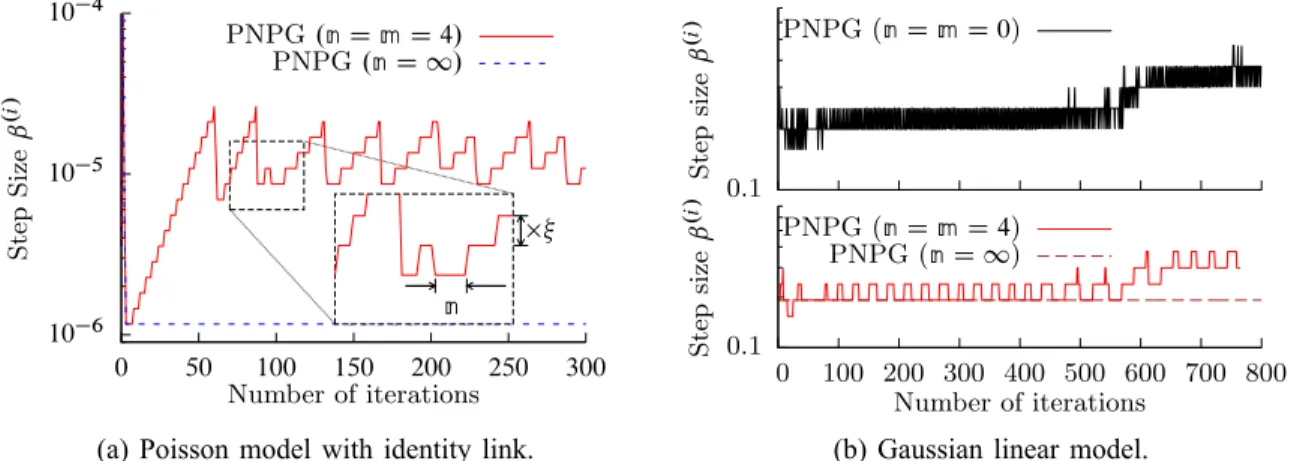
10 6 10 5 10 4 0 50 100 150 200 250 300 Step Size ˇ .i / Number of iterations PNPG.nDmD4/ PNPG.nD 1/ n
(a) Poisson model with identity link.
0.1 0.1 0 100 200 300 400 500 600 700 800 Step size ˇ .i / PNPG (nDmD0) Step size ˇ .i / Number of iterations PNPG (nDmD4) PNPG (nD 1)
(b) Gaussian linear model.
Fig. 1: Step sizes ˇ.i / as functions of the number of iterations for Poisson and Gaussian linear models.
Because of its iterative nature, (20e) is inexact; this inexactness can be modeled as
x.i / Ñ".i / proxˇ.i /ur xx.i / ˇ.i /rL.xx.i //
(24) where ".i / quantifies the precision of the PG step in Iteration i.
If we remove the convex-set constraint by settingC DRp, iteration (20a)–(20e) reduces to the Nesterov’s proximal-gradient iteration with adaptive step size that imposes signal sparsity only in the analysis form
(termed NPGS); see Section V-B for an illustrative comparison between NPGS and PNPG.
We now extend [16, Lemma 2.3] to the inexact proximal operation:
Lemma 1: Assume convex and differentiable NLL L.x/ and convex .x/, and consider an inexact PG step (24) with step size ˇ.i / that satisfies the majorization condition (21). Then,
f .x/ f .x.i // 1
2ˇ.i /
kx.i / xk22 kxx.i / xk22 .".i //2
(25) for all i 1 and any x 2Rp.
Proof: See Appendix A.
Lemma 1 is general and algorithm independent, because xx.i / can be any value indomL and we have used only the fact that step size ˇ.i / satisfies the majorization condition (21), rather than depending on specific details of the step-size selection. We use this result to establish the monotonicity property in Proposition 3 and to derive and analyze our accelerated PG scheme.
A. Restart and Monotonicity
If f .xx.i // > f .x.i // > f .x.i 1// or xx.i / 2C ndomL, set
re-evaluate (20b)–(20e), and refer to this action as function restart [40] or domain restart, respectively; see Algorithm 1. Function and domain restarts ensure that the PNPG iteration is monotonic and xx.i / remains withindomf as long as the projected initial value is withindomf:f .PC.x.0/// <C1. In this paper, we employ PNPG iteration with restart, unless specified otherwise (e.g., in Theorems 1 and 2 in Section IV).
Proposition 3 (Monotonicity): The inexact PG step (24) is monotonic:
f .x.i //f .xx.i // (27a)
if it is sufficiently accurate such that
".i / kxx.i / x.i /k2: (27b)
Hence, the PNPG iteration with restart and inexact PG steps (24) is non-increasing:
f .x.i //f .x.i 1// (28)
if (27b) holds for all i.
Proof: (27a) is straightforward by plugging x D xx.i / and (27b) into (25).
If there is no restart in Iteration i, the objective function has not increased. If there is a restart,.i 1/ D1, (20d) simplifies to xx.i / DPC.x.i 1//Dx.i 1/, and monotonicity follows due to xx.i / Dx.i 1/.
To establish the monotonicity in Proposition 3, the step size ˇ.i / need satisfy only the majorization condition (21).
B. Adaptive Step Size
Define the step-size adaptation parameter
2.0; 1/: (29)
We propose the following adaptive scheme for selectingˇ.i /:
i) if there have been no step-size backtracking events or increase attempts for n consecutive iterations (i n to i 1), start with a larger step size:
x
ˇ.i / Dˇ.i 1/= (increase attempt); (30a)
otherwise start with
x
ˇ.i / Dˇ.i 1/I (30b)
ii) (backtracking search) select
where0ti tMAXis the smallest integer such that (30c) satisfies (21);backtracking eventcorresponds
to ti > 0.
iii) if max.ˇ.i /; ˇ.i 1// <ˇx.i /, increase n by a nonnegative integer m:
n nCm: (30d)
We select the initial step size ˇx.1/ using the BB method [41]. If there has been an attempt to change the step size in any of the previous n consecutive iterations, we start the backtracking search ii) with the step size from the latest completed iteration. Consequently, ˇ.i / will be approximately piecewise constant as a function of the iteration index i; see Fig. 1, which shows the evolutions ofˇ.i / for measurements following the Poisson generalized linear and Gaussian linear models corresponding to Figs. 4a and 6b in Sections V-A and V-B. To reduce sensitivity to the choice of the tuning constant n, we increase its value by m if there is a failed attempt to increase the step size in Iteration i; i.e., ˇx.i /> ˇ.i 1/ and ˇ.i / <ˇx.i /.
The adaptive step-size strategy keeps ˇ.i / as large as possible subject to (21), which is important not only because the signal iterate may reach regions ofL.x/with different local Lipschitz constants, but also because of the varying curvature of L.x/in different updating directions. For example, a (backtracking-only) PG-type algorithm with non-adaptive step size would fail or converge very slowly if the local Lipschitz constant of
rL.x/ decreases as the algorithm iterates, because the step size will not adjust and track this decrease; see also Section V, which demonstrates the benefits of step-size adaptation.
Setting n D C1 corresponds to step-size backtracking only. A step-size adaptation scheme with n D
m D0 initializes the step-size search aggressively, with an increase attempt (30a) in each iteration.
C. Inner-Iteration Warm Start and Convergence Criteria
For .x/in (4), the inner iteration solves (20e) using the dual problem (10b). Denote byp.i;j / the iterates of the dual variable p in the jth inner iteration step within Iteration i; this inner iteration solves (20e) using (10b). The initial p.i;0/ is the latest p from Iteration i 1, which is referred to in [14] as the warm restart. (The variable metric inexact line-search algorithm (VMILA) [19] also uses warm restart.)
We consider two convergence criteria. The first tracks local variation of the signal iterates (23b):
kx.i;j / x.i;j 1/k pı.i 1/ (31a)
where is a tuning constant.
The second duality-gap–based criterion relies on the result in Proposition 2 to guarantee that ..k/".k//2
decreases at a rate of O.k q/ within each iteration segment without restart; this guarantee allows us to control the decrease of the convergence-rate upper bound in Section IV. Denote by i the iteration index of the latest restart prior to (and excluding) Iteration i (i 1); set its initial value 1 D 0. We select the
duality-gap based inner-iteration convergence criterion as (see also (10e) and (11)) G.i;j / ˇ.i /u xy.i;j / .i i/q..i //2 (31b)
where is a tuning constant and q is the accuracy rate [14]. Here, G.i;j / and y
x.i;j / are the duality gap
Ga;.p.i;j // and xya;.p.i;j // in (11) and (10e) (respectively) for a D xx.i / ˇ.i /rL.xx.i // and D ˇ.i /u. Without restart (i.e.,i 0) and step-size adaptation, (31b) reduces to the inner-iteration convergence criterion in [14, Sec. 6.1].
Adjusting . We use in (31a)–(31b) to trade off accuracy and speed of the inner iterations. If f .x.i // >
max f .x.i 1//; f .xx.i // indicating that the monotonicity condition (27b) does not hold, we decrease by an order of magnitude (10 times) and re-evaluate (20a)–(20e).
IV. Convergence Analysis
We now bound the convergence rate of the PNPG method without restart.
Theorem 1 (Convergence of the Objective Function): Assume that the NLL L.x/ is convex and differ-entiable, .x/ is convex, the closed convex set C satisfies
C domL (32)
(implying no need for domain restart), and the momentum tuning constants are within the range (22). Consider the PNPG iteration without restart with the inexact PG step (24) in place of (20e). The convergence rate of the PNPG iteration is bounded as follows: for k1,
.k/ kx .0/ x?k22CE.k/ 2ˇ.k/..k//2 (33a) 2 kx .0/ x?k22CE.k/ 2 pˇ.1/ CPkiD1 p ˇ.i /2 (33b)
where x? is a minimum point of f .x/ and
.k/,f .x.k// f .x?/ (34a) E.k/ , k X iD1 ..i /".i //2 (34b)
are the centered objective function and the cumulative error term, which accounts for the inexact PG steps, respectively.
Proof: See Appendix A for the proof of (33a); then, to obtain (33b), use .k/ q ˇ.k/ 1 q ˇ.k/C.k 1/qˇ.k 1/ (35a) 1 k X iD2 q ˇ.i / C.1/ q ˇ.1/ (35b)
for all k > 1, where (35a) follows from the definitions ofB.k/ and.k/in (20a) and (20b), and (35b) follows by repeated application of the inequality (35a) with k replaced by k 1; k 2; : : : ; 2.
Theorem 1 shows that better initialization, smaller proximal-mapping approximation error, and larger step sizes .ˇ.i //kiD1 help lower the convergence-rate upper bounds in (33). This result motivates our step-size adaptation with the goal of maintaining large .ˇ.i //kiD1; see Section III-B. To derive this theorem, we have used only the fact that the step sizeˇ.i / satisfies the majorization condition (21), rather than taking advantage of specific details of the step-size selection.
To minimize the upper bound in (33a), we can select.i /to satisfy (A16b) with equality, which corresponds to 2;1=4.i / in (20b), on the boundary of the feasible region in (22). By (35a), pˇ.k/.k/
and the denominator of the bound in (33a) are strictly increasing sequences. The upper bound in (33b) is not a function of b and is minimized with respect to for D2, given the fixed step sizes .ˇ.i //C1
iD0.
Corollary 1: Under the assumptions of Theorem 1, the convergence of PNPG iterationx.k/without restart is bounded as follows: .k/2kx .0/ x? k22CE.k/ 2.kC1/2ˇ min (36a) for k1, provided that
ˇmin, C1 min kD1ˇ .k/ > 0: (36b) Proof: Use (33b) and the fact that pˇ.1/CPk
iD1 p
ˇ.i / .k C1/pˇ
min.
The assumption (36b) is implied by, and weaker than, the Lipschitz continuity ofrL.x/; indeed,ˇmin> =L
if rL.x/ has a Lipschitz constant L; see also (29).
According to Corollary 1, the PNPG iteration attains the O.k 2/convergence rate as long as the step size
ˇ.i / is bounded away from zero (see (36b)) and the cumulative error term (34b) converges:
E.C1/
, lim
k!C1E .k/
<C1 (37)
which requires that ..k/".k//2 decreases at a rate of O.k q/ with q > 1. This condition, also key for establishing convergence of iterates in Theorem 2, motivates us to use decreasing convergence criteria (31a)– (31b) for the inner proximal-mapping iterations, where (31b) guarantees (37) upon choosing an appropriate
q.
in PG schemes. By recursively generating a function sequence that approximates the objective function, [14] gives an asymptotic analysis of the effect of ".i / on the convergence rate of accelerated PG methods with
inexact proximal mapping. However, no explicit upper bound is provided for .k/. Schmidt et al. [13]
provide convergence-rate analysis and an upper bound on .k/, but their analysis does not apply here
because it relies on fixed step-size assumption, uses different form of acceleration [13, Prop. 2], and has no convex-set constraint. Bonettini et al. [19] analyze the inexactness of proximal mapping but for proximal variable-metric/scaling methods with O.k 1/convergence rate for the objective function.
We now establish convergence of the PNPG iterates. Theorem 2 (Convergence of Iterates): Assume that 1) the conditions of Theorem 1 hold;
2) E.C1/ exists: (37) holds;
3) the momentum tuning constants .; b/ satisfy
> 2; b 2 Œ0; 1=2I (38)
4) the step-size sequence .ˇ.i //C1iD1 is bounded within the range Œˇmin; ˇmax, for ˇmin > 0.
Consider the PNPG iteration without restart with the inexact PG step (24) in place of (20e). Then, the sequence of PNPG iterates x.i / converges to a minimizer of f .x/.
Proof: See Appendix B.
Observe that Assumption 3 requires a narrower range of .; b/ than (22): indeed (38) is a strict subset of (22). The intuition is to leave a sufficient gap between the two sides of (A16a) so that their difference becomes a quantity that is roughly proportional to the growth of .i /, which is important for proving the
convergence of signal iterates [42]. Although the momentum term (20b) with D2 is optimal in terms of
minimizing the upper bound on the convergence rate (see Theorem 1), it appears difficult or impossible to prove convergence of the signal iterates x.i / for this choice of because, in this case, the gap between the two sides of (A16a) is upper-bounded by a constant.
Iterate convergence results in [10, 42, 43] apply to momentum-accelerated methods that require non-increasing step-size sequences and do not adjust to the local curvature of the NLL. Aujol and Dossal [43] analyze both the convergence of the objective function and the iterates with inexact proximal operator for
B.1/ D 1 and n D 1, i.e., with decreasing step size only, and for a different (less aggressive) .i / than ours in (20b). Bonettini et al. use the ideas from [42] to establish convergence of iterates for their variable-metric/scaling approach in [10], but this analysis does not account for inexact proximal steps.
A. O.k 2/ Convergence Acceleration Approaches
A few variants that accelerate the PG method achieve the O.k 2/ convergence rate [18, Sec. 5.2]. One competitor proposed by Auslender and Teboulle in [20, Sec. 5] and restated in [18] where it was referred to
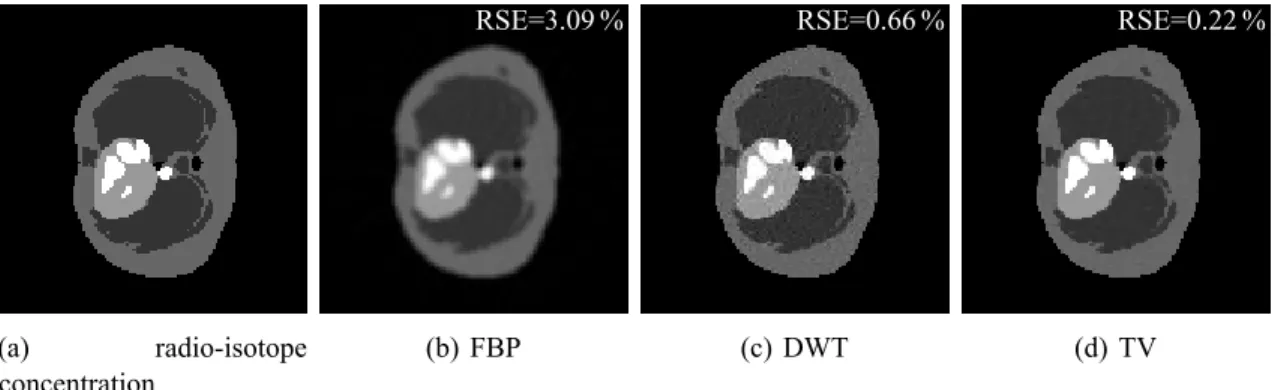
(a) radio-isotope concentration RSE=3.09 % (b) FBP RSE=0.66 % (c) DWT RSE=0.22 % (d) TV
Fig. 2: (a) True emission image and (b)–(d) the reconstructions of the emission concentration map.
as AT, replaces (20d)–(20e) with
x x.i / D1 1 .i / x.i 1/C 1 .i /xz .i 1/ (39a) z x.i / Dprox.i /ˇ.i /ur xz.i 1/ .i /ˇ.i /rL.xx.i // (39b) x.i / D1 1 .i / x.i 1/C 1 .i /xz .i / (39c) where .i /D2;1=4.i / in (20b). Here, ˇ.i / in the TFOCS implementation [18] is selected using the aggressive
search with nDmD0.
All intermediate signals in (39a)–(39c) belong to C and do not require projections onto C. However,
as .i / increases with i, step (39b) becomes unstable, especially when an iterative solver is needed for its proximal operation. To stabilize its convergence, AT relies on periodic restart by resetting .i / using (26) [18]. However, the period of restart is a tuning parameter that is not easy to select. For a linear Gaussian model, this period varies according to the condition number of the sensing matrix ˆ[18], which is generally unavailable and not easy to compute for large-scale problems. For other models, there are no guidelines how to select the restart period.
In Section V, we show that AT converges slowly compared with PNPG, which justifies the use of projection onto C in (20d) and (20d)–(20e) instead of (39a)–(39c). PNPG usually runs uninterrupted (without restart) over long stretches and benefits from Nesterov’s acceleration within these stretches, which may explain its better convergence properties compared with AT. PNPG may also be less sensitive than AT to proximal-step inaccuracies; we have established convergence-rate bounds for PNPG that account for inexact proximal steps (see (33) and (36a)), whereas AT does not yet have such bounds, to the best of our knowledge.
1) Relationship with FISTA: The PNPG method is a generalized FISTA [16] that accommodates convex constraints, more general NLLs,2 and (increasing) adaptive step size. In contrast with PNPG, FISTA has a
non-increasing step size ˇ.i /, which allows for setting B.i /
D1 in (20b) for alli (see Appendix A-II); upon setting .; b/D.2; 1=4/, this choice yields the standard FISTA (and Nesterov’s [15]) update. Convergence of signal iterates has not been established for FISTA with.; b/D.2; 1=4/[44]. Theorem 2 comes close to this
goal because it establishes convergence of iterates of PNPG and corresponding FISTA for .; b/ arbitrarily close to .2; 1=4/.
The method in [10] is a variable-metric/scaling version of FISTA with projection of the extrapolation step to account for the convex constraints. [21] analyzes a version of FISTA where the (decreasing) step size is adjusted using a condition in [45] different from the majorization condition (21), and establishes objective-function convergence under the assumption that the step size is lower bounded. As FISTA, [10] and [21] do not adapt the step size and hence do not adjust to the local curvature of the NLL.
V. Numerical Examples
We now evaluate our proposed algorithm by means of numerical simulations. We adopt the nonnegative C
in (2) and the`1-norm sparsifying penalty in (4). The PNPG iterations with the local-variation and duality-gap inner convergence criteria (31a) and (31b) are labeled PNPG and PNPGd, respectively.
All iterative methods that we compare use the convergence criterion (23a) with
D10 9 (40)
and have the maximum number of iterations ImaxD104. In the presented examples, PNPG uses momentum
tuning constants .; b/ D .2; 1=4/ and adaptive step-size parameters n D 4 (unless specified otherwise),
m D n, D0:8, inner-iteration convergence constants D10 2 and .;q/D .1; 1:0001/ for PNPG and
PNPGd(respectively), and maximum number of inner iterationsJmax D1000. Here, PNPGd usesq D1:0001
with goal to guarantee (37).
We apply the AT method (39) implemented in the TFOCS package [18] with adaptive step size and a periodic restart every 200 iterations (tuned for its best performance) and our proximal mapping. Our inner convergence criteria (31b) cannot be implemented in the TFOCS package (i.e., it require editing its code). Hence, we select the proximal mapping that has a relative-error inner convergence criterion
kp.i;j / p.i;j 1/k2 0kp.i;j /k2; (41a) where p.i;j / is the dual variable employed by the inner iterations. This relative-error inner convergence criterion is easy to incorporate into the TFOCS software package [18] and is already used by the SPIRAL package; see [46]. Here, we select
0D10 6 (41b)
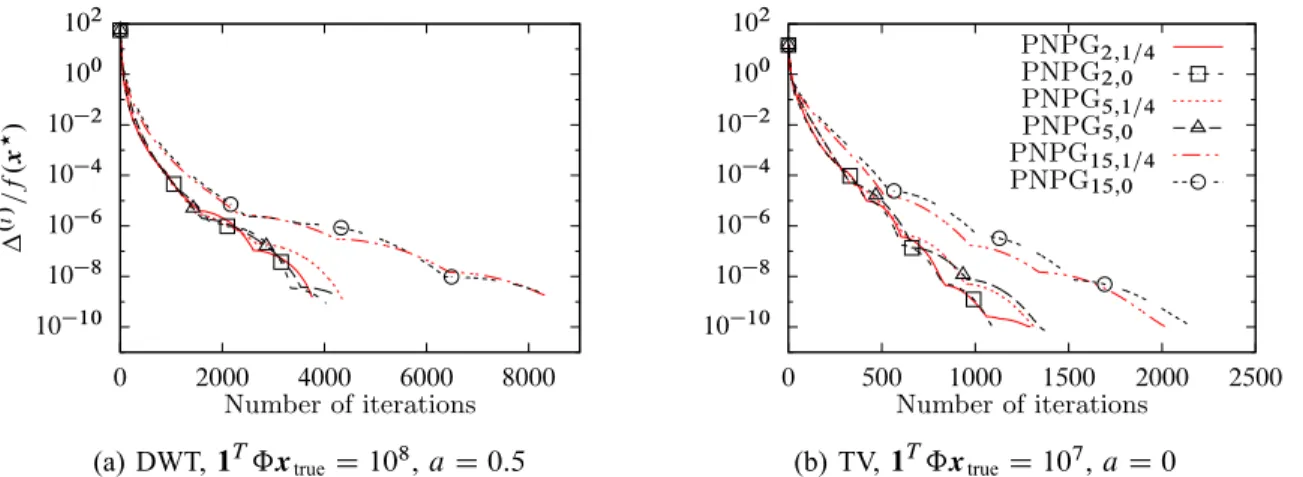
10 10 10 8 10 6 10 4 10 2 100 102 0 2000 4000 6000 8000 .i /=f . x ?/ Number of iterations (a) DWT,1TˆxtrueD108,aD0:5 10 10 10 8 10 6 10 4 10 2 100 102 0 500 1000 1500 2000 2500 Number of iterations PNPG2;1=4 PNPG2;0 PNPG5;1=4 PNPG5;0 PNPG15;1=4 PNPG15;0 (b) TV,1TˆxtrueD107,aD0
Fig. 3: Normalized centered objectives as functions of the number of iterations for (a) DWT and (b) TV regularizations.
We apply the CP approach based on [23, Sec. 7.5]:
z prox1FzC1ˆxx (42a) p PuH.pC2‰Hxx/ (42b) x x 2PC x ˆTzCRe.‰p/ x (42c) x .xxCx/=2 (42d)
obtained by splitting the objective function (3a) into the sum of F .ˆx/Cuk‰Hxk1 and IC.x/, where the first summand is a convex lower semicontinuous function of ŒˆH ‰Hx and F .ˆx/ D L.x/. In our examples in Sections V-A and V-B,F .y/and its convex conjugateF.z/have analytical proximal operators [23, Sec. 7.4]; hence, CP does not require an inner iteration. In the original CP algorithm in [27], Chambolle
and Pock select 1 D 2 D . However, when the difference between kˆk2 and k‰k2 becomes large, it
is hard to find tuning constants of the form .1; 2; / D .; ; / that ensure fast convergence of the CP
algorithm, which is why we do not impose 1 D2 D here. Another version of CP can be obtained by
associating the regularization parameter u with ‰ instead of the `1-norm function, which leads to replacing
uH with H and ‰; ‰H with u‰; u‰H, respectively, in (42). In this paper, we adopt the version of CP in
(42).
All the numerical examples were performed on a Linux workstation with an Intel Xeon CPU E31245 (3.30 GHz) and 8 GB memory. The operating system is Ubuntu 14.04 LTS (64-bit). The Matlab implementation of the proposed algorithms and numerical examples is available [47].
A. PET Image Reconstruction from Poisson Measurements
In this example, we adopt the Poisson GLM (16a) with identity link in (17). Consider PET reconstruction
of the 128 128 concentration map x in Fig. 2a, which represents simulated radiotracer activity in the
model the attenuation of the gamma rays [35] and compute the sensing matrix ˆ in this application. We collect the photons from 90 equally spaced directions over 180°, with 128 radial samples in each direction. Here, we adopt the parallel strip-integral matrix [48, Ch. 25.2] and use its implementation in the Image Reconstruction Toolbox (IRT) [49] with sensing matrix
ˆDwdiag expı. Cc/ (43)
where c is a known vector generated using a zero-mean independent, identically distributed (i.i.d.) Gaussian sequence with variance 0:3 to model the detector efficiency variation; w > 0 is a known scaling constant controlling the expected total number of detected photons due to electron-positron annihilation; and1T E.y b/D1Tˆx, which is a signal-to-noise ratio (SNR) measure. Assume that the background radiation, scattering
effect, and accidental coincidence combined lead to a known (generally nonzero) intercept term b in the
Poisson GLM (17). The elements of the intercept term have been set to a constant equal to 10 % of the sample mean of ˆxtrue: bD.1Tˆxtrue/=.10N /1.
The above model, choices of parameters in the PET system setup, and concentration map have been adopted
from IRT [49, emission/em_test_setup.m].
Here, we consider the DWT and isotropic TV sparsifying transforms. We use the 2-D Haar DWT with
6 decomposition levels and a full circular mask [50] to construct a sparsifying dictionary matrix ‰ 2
R12 44914 056 with orthonormal rows, i.e., ‰‰T
D I, which allows efficient inner iteration. We compare
the filtered backprojection (FBP) [35] and PG methods that aim at minimizing (3) with nonnegative C in
(2) and DWT and TV sparsifying transforms.
We implemented SPIRAL with TV penalty using the centered NLL term (16a), which improves the numerical stability compared with the original code in [46]. We do not compare with SPIRAL that uses DWT penalty because its inner iteration for the proximal step requires a square orthogonal ‰(see [4, Sec. II-B]), which is not the case here. We also compare with VMILA [19, 51] with both DWT and TV penalties and its default tuning constants, which yield good performance; hence VMILA is insensitive to tuning.
In this example, we adopt the following form of the regularization constant u:
uD10a; (44)
vary a in the range Π6; 3 with a grid size of 0.5, and search for the reconstructions with the best average relative square error (RSE) performance; here, RSE D kyx xtruek22=kxtruek22, where xtrue and xy are the
true and reconstructed signals, respectively. All iterative methods were initialized by FBP reconstructions implemented by IRT [49].
Figs. 2b-2d show reconstructions and corresponding RSEs for one random realization of the noise and detector variation c, with the expected total annihilation photon count (SNR) equal to 108; the optimal a is
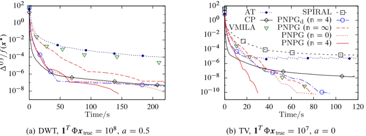
10 8 10 6 10 4 10 2 100 102 0 50 100 150 200 .i /=f . x ?/ Time/s (a) DWT,1TˆxtrueD108,aD0:5 10 10 10 8 10 6 10 4 10 2 100 102 0 20 40 60 80 100 120 Time/s AT CP VMILA SPIRAL PNPGd.nD4/ PNPG.nD 1/ PNPG.nD0/ PNPG.nD4/ (b) TV,1TˆxtrueD107,aD0
Fig. 4: Normalized centered objectives as functions of the CPU time for (a) DWT and (b) TV regularizations.
they employ the same penalty: the TV sparsity penalty is superior to its DWT counterpart; see [9, Fig. 6] which shows average RSEs of different methods as functions of 1Tˆxtrue.
Figs. 3 and 4 show the normalized centered objectives .i /=f .x?/as functions of the number of iterations and CPU time for the DWT and TV signal sparsity regularizations and two random realizations of the noise and detector variation with different total expected photon counts. The legends in Figs. 3b and 4b apply to Figs. 3a and 4a as well. Fig. 3 examines the convergence of PNPG as a function of the momentum
tuning constants .; b/ in (22), using 2 f2; 5; 15g and b 2 f0; 1=4g. For small 5, there is no
significant difference between different selections and no choice is uniformly the best, consistent with [42]
which considers only b D 0 and non-adaptive step size. As we increase further ( D 15), we observe
slower convergence. In the remainder of this section, we use .; b/D.2; 1=4/.
To illustrate the benefits of step-size adaptation, we present in Fig. 4 the performance of PNPG (nD 1), which does not adapt to the local curvature of the NLL and has monotonically non-increasing step sizesˇ.i /, similar to FISTA. PNPG (nD4) outperforms PNPG (nD 1) because it uses step-size adaptation; see also Fig. 1a, which corresponds to Fig. 4a and shows that the step size of PNPG (n D 4) is consistently larger
than that of PNPG (n D 1). Initializing PNPG iterations by a vector close to 0 (rather than with FBP)
will lead to an even larger difference in convergence speed between PNPG (n D 1) and PNPG (n D 4).
The advantage of PNPG (n D 4) over the aggressive PNPG (n D 0) scheme is due to the patient nature
of its step-size adaptation, which leads to a better local majorization function of the NLL and reduces time spent backtracking. Indeed, if we do not account for the time spent on each iteration and only compare the
objectives as functions of the iteration index, then PNPG (n D 4) and PNPG (n D 0) perform similarly;
see [8, Fig. 4]. Although PNPG (n D 0) and AT have the same step-size selection strategy and O.k 2/
convergence-rate guarantees, PNPG (n D 0) converges faster; both schemes are further outperformed by
PNPG (nD4). Fig. 4b shows that SPIRAL, which does not employ PG step acceleration, takes at least three times longer than PNPG (nD4) to reach the same objective function.
−0.5 0 0.5 1 1.5 2 2.5 0 200 400 600 800 1000
(a) true signal
−0.5 0 0.5 1 1.5 2 2.5 0 200 400 600 800 1000 RSE=0.011 % (b) PNPG −0.5 0 0.5 1 1.5 2 2.5 0 200 400 600 800 1000 RSE=0.23 % (c) NPGS
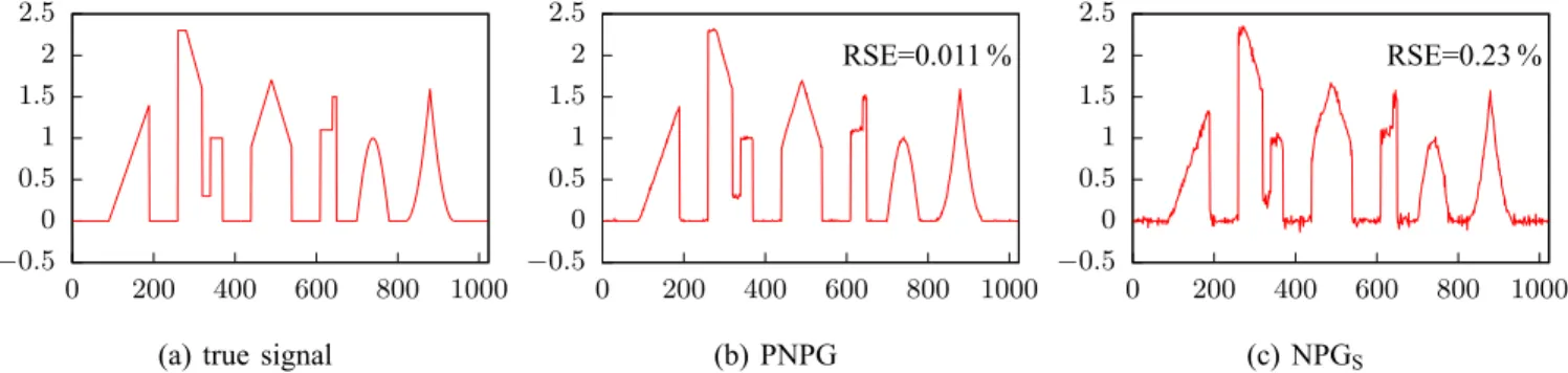
Fig. 5: Nonnegative skyline signal and its PNPG and NPGS reconstructions for N=pD0:34.
(41a); we observe a performance floor for AT in Fig. 4a as well. Reducing 0 in (41b) will lower this floor, at the cost of slowing down the two algorithms. This result justifies our convex-set projection in (20d) for the Nesterov’s acceleration step, shows the superiority of (20d) over AT’s acceleration in (39a) and (39c), and is consistent with the results in Section V-B.
PNPGd(nD4) employs the duality-gap–based inner convergence criterion (31b) with qD1:0001. Since
the goal of using (31b) is to guarantee (37), this inner criterion is more stringent and leads to slower overall performance of PNPGd(nD4) compared to PNPG (nD4). Indeed, if we do not account for the time spent
on each iteration and only compare the objectives as functions of the iteration index, then PNPGd(n D 4)
and PNPG (nD4) perform similarly with the former slightly better.
The CP method uses the following tuning constants carefully selected for this particular problem:.1; 2; /D
.10 6; 1; 10 3/and.
1; 2; /D.10 4; 1; 10 2/for the DWT and TV penalties, respectively. CP is sensitive
to tuning and a different selection of .1; 2; / can significantly slow down its convergence. Initially, CP converges quickly and then slows down as it approaches the optimum.
Considering its O.k 1/theoretical convergence rate, VMILA performs quite well, thanks to its use of the variable-metric/scaling approach.
B. Skyline Signal Reconstruction from Linear Measurements
We adopt the DWT sparsifying transform and linear measurement model with Gaussian noise in Section II-B where each column of the sensing matrixˆ are i.i.d. and drawn from the uniform distribution on unit sphere. Due to the widespread use of this measurement model, we can compare a wider range of methods than in the Poisson PET example in Section V-A.
We have designed a “skyline” signal of length p D 1024 by overlapping magnified and shifted triangle,
rectangle, sinusoid, and parabola functions; see Fig. 5a. We generate the noiseless measurements using y D
ˆxtrue. The DWT matrix ‰ is constructed using the Daubechies-4 wavelet with three decomposition levels
whose approximation by the 5 % largest-magnitude wavelet coefficients achievesRSED98%. We compare:
CP with the parameters 2 D 1 [27] and D 1 with 1 tuned separately for best performance in each experiment;3
linearly constrained gradient projection method [5], part of the SPIRAL toolbox [46] and labeled SPIRAL herein;
the GFB method [25] (see (4)):
z1 z1Cprox.ru=w/.2x z1 rrL.x// x (45a)
z2 z2CŒPC.2x z2 rrL.x// x (45b)
x wz1C.1 w/z2 (45c)
with rD1:9=kˆk22, D1, and w D0:5 tuned for best performance; and
the PDS method [28]: N z PŒ u;up.zC ‰Tx/ (46a) N x PC x rL.x/ ‰.2zN z/ (46b) z zCr.zN z/ (46c) x xCr.xN x/ (46d)
where we choose D 1=. C kˆk22=2/ and r D 2 0:5kˆk22. 1 / 1 with tuned for best
performance,4
all of which aim to solve the generalized analysis BPDN problem with a convex signal constraint. Here,
p0 D p, ‰ 2 Rpp is an orthogonal matrix (‰‰T
D ‰T‰
D I), and proxa D ‰T.‰Ta/ has a
closed-form solution (see (6c)), which simplifies the implementation of the GFB method ((45a), in particular); see the discussion in Section I. The other tuning options for SPIRAL, and AT are kept to their default values, unless specified otherwise.
We initialize the iterative methods by the approximate minimum-norm estimate:x.0/ DˆTŒE.ˆˆT/ 1y D
N ˆTy=p and select the regularization parameter u as
u D10aU; U ,k‰TrL.0/k1 (47)
where a is an integer selected from the interval Π9; 1 and U is an upper bound on u of interest. Indeed,
the minimum point x? reduces to 0 ifu U [38, Sec. II-D].
As before, PNPG (n D 4) and PNPG (n D 0) converge at similar rates as functions of the number of
iterations. However, due to the excessive attempts to increase the step size at every iteration, PNPG (nD0) spends more time backtracking and converges at a slower rate as a function of CPU time compared with
3We select1
D2 as in [27] becausekˆk2andk‰k2 have approximately the same scale in this example.
4These choices ofandrare at the boundary of the convergence region in [28, Th. 3.1]. We have searched forandrinside this convergence
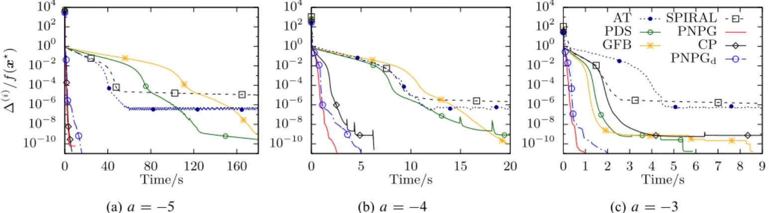
10−10 10−8 10−6 10−4 10−2 100 102 104 0 40 80 120 160 ∆ ( i ) /f ( x ⋆ ) Time/s (a) aD 5 10−10 10−8 10−6 10−4 10−2 100 102 104 0 5 10 15 20 Time/s (b)aD 4 10−10 10−8 10−6 10−4 10−2 100 102 104 0 1 2 3 4 5 6 7 8 9 Time/s AT PDS GFB SPIRAL PNPG CP PNPGd (c) aD 3
Fig. 6: Normalized centered objectives as functions of CPU time for normalized numbers of measurements
N=p D0:34 and different regularization constants a.
PNPG (n D4); see also Fig. 1b which corresponds to Fig. 6b and shows the step sizes as functions of the
number of iterations for aD 4 and N=pD0:34. Hence, we present only the performances of PNPG with
nD4 in this section.
Fig. 5 shows the advantage brought by the convex-set nonnegativity signal constraints (2). Figs. 5b and 5c
present the PNPG .a D 5/ and NPGS .a D 4/ reconstructions from one realization of the linear
measurements with N=p D 0:34 and a tuned for the best RSE performance. Recall that NPGS imposes
signal sparsity only. Here, imposing signal nonnegativity significantly improves the overall reconstruction and does not simply rectify the signal values close to zero.
Fig. 6 presents the normalized centered objectives .i /=f .x?/ as functions of CPU time for a random
realization of the sensing matrix ˆ with normalized numbers of measurements N=p D 0:34 and several
different regularization constants a. (For the GFB method, we compute the normalized centered objectives using PC.x.i // instead of x.i / in (34a) because its x.i / may be outside C.) The legend in Fig. 6c applies also to Figs. 6a and 6b. To achieve good performance, CP and PDS need to be manually tuned for each
a. CP and PDS have optimal 1 D 2 equal to 0:01; 0:1; 1 and 0:0026; 0:026; 2:6 for a D 5; 4; 3,
respectively.
PNPG and PNPGd have the steepest descent rate, followed by PNPGd. AT and SPIRAL reach the
performance floor around the relative precision of 10 6 due to their fixed inner convergence criterion in (41a). The GFB and primal-dual methods, PDS and CP, are sensitive to the selection of the tuning constants. After a careful selection of the tuning constants, CP performs exceptionally well in Figs. 6a and 6b. The performance of GFB is affected significantly by the value of the regularization parameter a.
VI. Conclusion
We developed a fast algorithm for reconstructing sparse signals that belong to a closed convex set by employing a projected proximal-gradient scheme with Nesterov’s acceleration, restart, and adaptive step size. We applied the PNPG method to construct one of the first Nesterov-accelerated proximal-gradient
reconstruction algorithm for Poisson compressed sensing. We presented integrated derivation of the proposed algorithm and convergence-rate upper bound that accounts for inexactness of the proximal operator and also proved convergence of iterates. Our PNPG approach is computationally efficient compared with other state-of-the-art methods.
Appendix A
Derivation of Acceleration (20a)–(20d) and Proofs of Lemma 1 and Theorem 1
We first prove Lemma 1 and then derive the acceleration (20a)–(20d) and prove Theorem 1. Proof of Lemma 1: According to Definition 1 and (24),
ur.x/ur.x.i //C.x x.i //Thxx .i / x.i / ˇ.i / rL.xx .i //i .".i //2 2ˇ.i / (A1a)
for any x 2Rp. Moreover, due to the convexity of L.x/,
L.x/L.xx.i //C.x xx.i //TrL.xx.i //: (A1b)
Summing (A1a), (A1b), and (21) completes the proof.
The following result from [34, Prop. 3.2.1 in Sec. 3.2] states that the distance between x and y can be reduced by projecting them onto a closed convex set C.
Lemma 2 (Projection theorem): The projection mapping onto a nonempty closed convex set C Rp is nonexpansive
kPC.x/ PC.y/k22 kx yk 2
2 (A2)
for all x;y 2 Rp.
We now derive the projected Nesterov’s acceleration step (20b)–(20d) with the goal of selecting thexx.i / in the proximal step (20e) that achieves the convergence rate of O.k 2/. This derivation and convergence-rate
proof are inspired by—but are more general than—[16]. We start from (25) with x replaced byx Dx? and
x Dx.i 1/, .i / kx .i / x? k2 2 kxx .i / x?k22 .".i //2 2ˇ.i / (A3a) .i 1/ .i / ı .i / kxx.i / x.i 1/k22 .".i //2 2ˇ.i / (A3b)
and design two coefficient sequences a.i / > 0 and b.i / > 0 that multiply (A3a) and (A3b), respectively, which ultimately leads to (20a)–(20d) and the convergence-rate guarantee in (33a).
Consider sequences a.i / > 0 and b.i / > 0. Multiply them by (A3a) and (A3b), respectively, add the resulting expressions, and multiply by ˇ.i / to obtain
2ˇ.i /c.i /.i /C2ˇ.i /b.i /.i 1/ 1 c.i / c.i /x.i / b.i /x.i 1/ a.i /x?22 1 c.i /kc .i / x x.i / b.i /x.i 1/ a.i /x?k22 c.i /.".i //2 Dc.i /t.i / tN.i / .".i //2 (A4) where c.i / ,a.i /Cb.i / (A5a) t.i / ,kx.i / z.i /k22; tN .i / ,kxx.i / z.i /k22 (A5b) z.i / , b .i / c.i /x .i 1/ C a .i / c.i /x ? : (A5c)
We arranged (A4) using completion of squares so that the first two summands are similar (but with opposite signs), with the goal of facilitating cancellations as we sum overi. Since we have control over the sequences
a.i / and b.i /, we impose the following boundary conditions for i 1:
c.i 1/t.i 1/ c.i /tN.i / (A6a)
.i / 0 (A6b)
where
.i /,ˇ.i /c.i / ˇ.iC1/b.iC1/: (A7)
Now, apply the inequality (A6a) to the right-hand side of (A4):
2ˇ.i /c.i /.i /C2ˇ.i /b.i /.i 1/ c.i /t.i / c.i 1/t.i 1/
c.i /.".i //2 (A8a)
and sum (A8a) over i D1; 2; : : : ; k, which leads to summand cancellations and
2ˇ.k/c.k/.k/C2ˇ.1/b.1/.0/ 2 k 1 X iD1 .i /.i / c.0/t.0/ k X iD1 c.i /.".i //2 (A8b)
Now, due to .i /.i / 0 (see (34a) and (A6b)), the inequality (A8b) leads to
.k/ 2ˇ
.1/b.1/.0/
Cc.0/t.0/CPikD1c.i /.".i //2
2ˇ.k/c.k/ (A9)
with simple upper bound on the right-hand side, thanks to summand cancellations facilitated by the assump-tions (A6).
As long as ˇ.k/c.k/ grows at a rate ofk2 and the inexactness of the proximal mappings leads to bounded
Pk iD1c
.i /.".i //2
, the centered objective function .k/ can achieve the desired bound decrease rate of 1=k2. In the following section, we show how to satisfy (A6a), which will lead to the projected momentum acceleration step (20d). We approach the constraints (A6a) by first aiming to meet them with equality, which is possible in the absence of the convex-set constraint (C DRp). We then use the nonexpansiveness of the convex-set projection to construct a.i / and b.i / that satisfy (A6a) with inequality in the general case where the convex-set constraint is present. Finally, we show how to satisfy (A6b), which will allow us to construct the recursive update of .i / in (20b) and verify the allowed range of momentum tuning constants in (22).
I Satisfying Conditions (A6)
a) Imposing equality in(A6a): (A6a) holds with equality for alli and anyx?when we choosexx.i / D yx.i /
that satisfies
p
c.i 1/.x.i 1/ z.i 1//Dpc.i /.xy.i / z.i //: (A10) Now, (A10) requires equal coefficients multiplying x? on both sides; thus a.i /=pc.i /
D1=wfor alli, where
w> 0 is a constant (not a function of i), which implies c.i / D w2.a.i //2
and b.i / Dw2.a.i //2 a.i / ; see also (A5a). Upon defining
.i / ,w2a.i / (A11a)
we have
w2
c.i / D..i //2I w2
b.i / D..i //2 .i /: (A11b)
Plug (A11) into (A10) and reorganize to obtain the following form of momentum acceleration:
y
x.i / Dx.i 1/C‚.i /.x.i 1/ x.i 2//: (A12) Although xx.i / D yx.i / satisfies (A6a), it is not guaranteed to be within domL; consequently, the proximal-mapping step for this selection may not be computable.
b) Selecting xx.i / 2C that satisfies(A6a): We now seek xx.i / withinC that satisfies the inequality (A6a). Since x.i 1/and x? are inC,z.i / 2C by the convexity ofC; see (A5c). According to Lemma 2, projecting
(A12) onto C preserves or reduces the distance between points. Therefore,
x
x.i / DPC.xy .i /
/ (A13)
belongs to C and satisfies the condition (A6a):
c.i 1/t.i 1/Dc.i /kyx.i / z.i /k22 (A14a)
c.i /kxx.i / z.i /k22 Dc.i /tN.i / (A14b)
where (A14a) and (A14b) follow from (A10) and by using Lemma 2, respectively; see also (A5b).
Without loss of generality, set w D 1 and rewrite and modify (A7), (A5b), and (A8b) using (A11) to
obtain .i / Dˇ.i /..i //2 ˇ.iC1/.iC1/..iC1/ 1/; i 1 (A15a) ..i //2t.i / D.i /x.i / ..i / 1/x.i 1/ x?22 (A15b) k 1 X iD1 .i /.i / 1 2 h ..0//2t.0/C k X iD1 ..i /".i //2i (A15c)
where (A15c) is obtained by discarding the negative term 2ˇ.k/..k//2.k/and the zero termˇ.1/.1/..1/ 1/.0/ (because .1/ D 1) on the left-hand side of (A8b). Now, (33a) follows from (A9) by using .0/ D .1/D1 (see (20b)), (A11), and (A15b) with i D0.
c) Satisfying (A6b): By substituting (A15a) into (A6b), we obtain the conditions
ˇ.i 1/..i 1//2 ˇ.i /..i //2 .i / (A16a) and interpret ..i //C1iD1 as the sequence of gaps between the two sides of (A16a); (A16a) implies
.i / 1=2C
q
1=4CB.i /..i 1//2: (A16b)
Comparing (20b) with (A16b) justifies the constraints in (22). II Connection to Convergence-Rate Analysis of FISTA in [16]
If the step-size sequence .ˇ.i // is non-increasing (e.g., in the backtracking-only scenario with nD C1), (20b) with B.i /
D 1 also satisfies the inequality (A16b). In this case, (33a) still holds but (33b) does not because (35) no longer holds. However, because B.i /
D1, we have .k/ .kC1/= and .k/2kx .0/ x?k22CE.k/ 2ˇ.k/.k C1/2 (A17)
which generalizes [16, Th. 4.4] to include the inexactness of the proximal operator and the convex-set projection.
Appendix B
Convergence of Iterates
To prove convergence of iterates, we need to show that the centered objective function .k/ decreases faster than the right-hand side of (33b). We introduce Lemmas 3 and 4 and then use them to prove Theorem 2. Throughout this Appendix, we assume that Assumption 1 of Theorem 2 holds, which justifies (A3) and (A16) as well as results from Appendix A that we use in the proofs.
Lemma 3: Under Assumptions 1–3 of Theorem 2,
C1 X iD1
.2.i / 1/ı.i / <C1: (B1)
Proof: By letting k! C1 in (A15c) and using (37), we obtain C1
X iD1
.i /.i / <C1: (B2)
For i 1, rewrite (A15a) using .i / expressed in terms of .iC1/ (based on (20b)):
.i / D ˇ .iC1/ . 2/.iC1/C.1 b2/= 2ˇ.iC1/.iC1/ (B3)
where the inequality in (B3) is due to b2 1 < 0; see Assumption 3. Apply nonexpansiveness of the
projection operator to (A3b) and use (A12) to obtain
2ˇ.i /..i 1/ .i //ı.i / .‚.i //2ı.i 1/ .".i //2I (B4) then multiply both sides of (B4) by ..i //2, sum over i D1; 2; : : : ; k and reorganize:
k 1 X iD1 .2.i / 1/ı.i /..0/ 1/2ı.0/ ..k//2ı.k/CE.k/ C2ˇ.1/.0/ 2ˇ.k/..k//2.k/C2 k 1 X iD1 %.i /.i / (B5a) E.k/C2ˇ.1/.0/C 4 2 k 1 X iD1 .i /.i / (B5b)
where (see (A15a))
%.i /,ˇ.iC1/..iC1//2 ˇ.i /..i //2 (B5c)
Dˇ.iC1/.iC1/ .i /; (B5d)