SLEEP SCORING
A NEURAL NETWORK APPROACH
Joan Marcual Medina
Advisor: Jimeng Sun
Contents
1 Abstract 4
2 Introduction 5
2.1 Motivation . . . 5
2.2 Objective . . . 7
3 State of the art 8 4 Background 10 4.1 KNN and Dynamic Time Warping . . . 10
4.2 Neural Networks . . . 11
4.3 Architectures . . . 12
4.3.1 Multi Layer Perceptron . . . 12
4.3.2 Convolution Neural Networks . . . 13
4.3.3 Fully convulutional Neural Networks . . . 15
4.3.4 Residual Neural Networks . . . 15
5 Dataset 18 6 Data preprocess 21 6.1 ECG . . . 22
6.2 EEG . . . 23
7 Experiments and results 24
7.1 Experimental setup . . . 24 7.2 ECG . . . 25 7.3 EEG . . . 27
1
Abstract
Sleep disorders tend to be undiagnosed due to the high costs associated with Polysomnography. Polysomnography requires patients to spend a night in a high paramedic system that records different biological signals. The high cost of this procedure is due to the paramedic equipment and the highly trained human labor scoring the sleep session. In this work, we explore two solutions using neural networks to solve this problem. The first one using only one EEG signal to automatically score the sleep session. In the second, we explore the possibility of doing all the procedure using only ECG, allowing the possibility of in-house diagnoses.
2
Introduction
2.1
Motivation
Sleep has been proven to play an important role in both physical and mental health. Good sleep expands our life span [5], protects us from cancer [4] and lowers the possibilities of stroke and heart attack [6]. It has also been proved that sleep improves our mental health, enhances our memory [25], and reduces the chances of suffering from dementia and depression [14]. In order to benefit of all of these qualities is not only enough to sleep a certain amount of hours, but it is also important to achieve a certain quality of sleep in those hours.
Sleep is classified in 5 states. REM (Rapid Eye Movement), NREM1 (No Rapid Eye movement), NREM2, NREM3. NREM1 and NREM2 are classically seen as light sleep and NREM3 and REM are classically seen as deep sleep. The distribution and the patterns of these categories during a sleep session are what determines its quality.
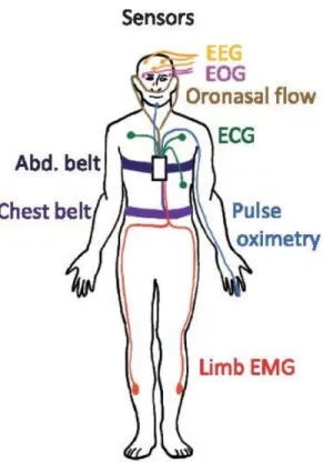
The normal procedure to acquire the categorization of a sleep session is the polysomnography (PSG) (Figure 1). Where the patient sleeps in a high paramedic system that records different biological signals being these ones: electroencephalogram (EEG), electrooculogram (EOG), electrocardio-gram (ECG), electromyoelectrocardio-gram (EMG), blood oxygenation, airflow, and res-piratory effort. After the sleeping session, highly trained technicians have to go through all the sleeping hours and manually classify it.
The present method has important drawbacks. Firstly, is a highly costly method, it requires both specialized equipment and highly trained experts. Secondly, is an intense human laborious work. Each sleep session requires in average 2 hours to be fully classified by the trained technicians. Last but not least, it requires an active approach from the patient in order to be diagnosed.
Figure 1: Polysomnography analysis
All the mentioned problems, make a diagnosis of sleep disorders a hard task. 50 to 70 million Americans are affected by chronic sleep disorders and intermittent sleep problems, the overwhelming majority of them undiagnosed and untreated [1]. Therefore, increasing their risk of premature deaths, de-creasing life spans, and life quality.
Sleeping analysis has been trying to be automated in different works [11] [19] [21]. Automation helps to mitigate the associated cost problem. However, the need to actively sleeping in a different and highly paramedic environment is still a persistent problem.
2.2
Objective
In this work, we explore two solutions for these problems. Our first solution is the automation of sleep staging using only one EEG channel. The current approach uses 6 channels in order to gather data for sleep analysis. The automation approach will eradicate the need of highly qualified technicians and therefore reduce the cost associated with the procedure. Reducing from 6 channels to 1 channel will reduce the cost to some extent. Besides, it will improve the patient experience in the analysis, reducing the number of paramedic devices attached to the patient creating a more comfortable environment for the test.
The second approach is using the ECG signal. This approach carries the same virtues as the first one, however, the real impact could be greater. With the rise of the use of wearable devices, a new opportunity for home diagnosis has been open. A full sleep classification with ECG signal alone has been shown to be a not feasible task. A more realistic approach is the classification of a lesser number of classes. The objective of this work would be to explore these possibilities. A lesser class classification would not be used for fine diagnosis, however, can serve the purpose of an in house detector of sleep disorders in an early stage.
Neural networks have been shown to excel in classification tasks [18] [15] [17]. They have been used in widely different areas, from text classification to image classification, achieving even better performance than humans in some cases [12]. In this work, we explore the state of the art neural net architectures to solve this problem.
3
State of the art
Manual sleeping staging is done over the polysomnographic (PSG) signals. PSG includes the following signals: electroencephalogram (EEG), electroocu-logram (EOG), and electromyogram (EMG) is recorded for muscle tone mon-itoring. Being EEG the most important signal and the first used to classify sleep stages in 1924 [22]. Being this process a highly labor-intensive task, its automation has been an area of research widely explored.
The first studies started in the early 70s [23] and have been evolving since then. With the rise of machine learning as a field of research, the area has been revisited several times with new different approaches. Some of the most relevant machine learning approaches are used KNN, GMM, decision trees, Random forest, and LDA, as learning techniques.
Gunes et al. 2010 [10] gathered 129 features using Welch spectral analysis from EEG signals. After that, they applied a feature reduction method based in K-means over the following statistics: minimum value, maximum value, standard deviation and mean. Finally, they applied a KNN classifier reaching a 71% accuracy.
Fraiwan et al. 2010 [7] engineered 21 features using the Continuous Wavelet Transform (CWT) time-frequency using three wavelets. After that, they applied Linear Discriminant Analysis. Once the projection was applied they used the nearest centroid as a classifier for the points in the new space. Using this method over the projection the accuracy gained was of 80%.
After that Fraiwan et al. 2012[8] explored the idea of using Random Forest as the classifier method. The features selected for this work were reduced to 7. The features were extracted using the Choi-Williams distribu-tion, Hilbert-Huang Transform, Renyi’s Entropy measures, and the already used CWT. Using this new method Fraiwan et al. improved their accuracy from 80% to 86%.
In the last decade, Artificial Neural Networks (ANN) have gained impor-tance as one of the most powerful classifiers. As a result, multiple works have explored the idea of applying distinct ANN architectures over ECG
signals in different classification tasks, arrhythmia classification, apnea de-tection, heart failure dede-tection, etc. The most relevant works are: Real-Time Patient-Specific ECG Classification [16] by Kiranyaz et. al 2016 and Ap-plication of stacked convolutional and long short-term memory network for accurate identification of CAD ECG signals [26] by Tan et al., 2017.
Kiranyaz et. al use a 1-D Convolutional Neural Net architecture to detect arrhythmias. Using this technique they achieved a 99% of accuracy in the MIT/BIH arrhythmia dataset [9]. Tan et al. used a long short-term memory neural network approach to identify coronary artery disease. The neural net approach also reached a 99% of accuracy for this task.
4
Background
4.1
KNN and Dynamic Time Warping
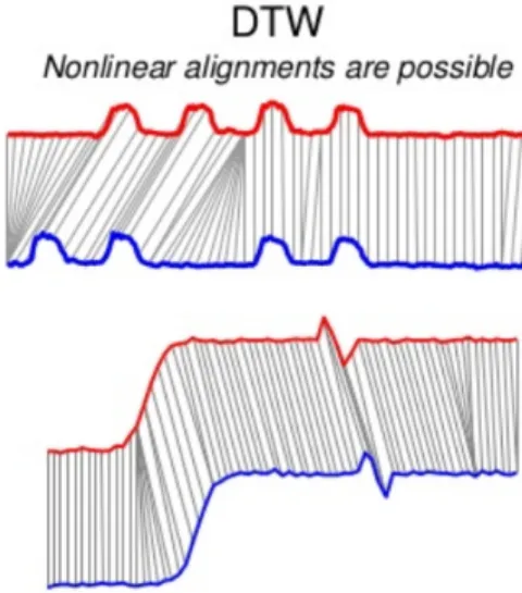
Figure 2: Euclidian distance vs DTW
The classic approach to classification of timeseries is K-Nearest Neighbors (KNN) using dynamic time warping as distance. KNN algorithm is a non-parametric supervised learning algorithm. KNN stores all the previously seen data samples, in this case, time series, and their respective labels. In order to predict an unseen data point KNN first computes the distance with each previously seen data point and the new one. After that, it takes the K nearest points or neighbors, being K a hyperparameter, and assigns the most popular class among the neighbors.
In most problems, the distance chosen for this task is the Euclidian dis-tance: D= n X i=0 q (T1i+T2i)2
The Euclidian distance is defined as the sum of distances between the same instants of time. The main problem of using this distance over time series is that is not robust against desynchronized series. The algorithm will totally fail to identify the same time series if both of them do not start at the same time and follow through at the same exact speed. This phenomenon can be seen in Figure 2. This problem makes the Euclidian distance totally incapable of generalizing and therefore is not advised to use it for time series classification.
As a response to these problems, Dynamic Time Warping (DTW) was proposed [3]. Dynamic Time Warping takes into account this problem and looks for the best fit between the data points of each time series (Figure 2). The pseudocode of DTW is the following one. We have decided to use KNN+DTW as a strong baseline for our work.
Algorithm 1 Dynamic Time Warping
1: procedure int DTWDistance(s: array [1..n], t: array [1..m])
2: DT W :=array[0..n],0..m] 3: for i←1 to N do 4: for j ←1 to M do 5: DT W[i, j] :=inf inity 6: DT W[0,0] := 0 7: for i←1 to N do 8: for j ←1 to M do 9: cost:=d(s[i], t[j]) 10: DT W[i, j] := cost + minimum(DT W[i − 1, j], DT W[i, j − 1], DT W[i−1, j−1]) return DTW[n, m]
4.2
Neural Networks
Neural networks are a set of layers, where a layer L is a parametric function. One layer li , such as i ∈ [1, L], is a set of nodes called neurons. A neuron is a small unit that compute one element of the layer’s output. Each layer l takes its input from the previous layer l-1 and applies a linear or non-linear function to it. The output of these functions is passed as input for
the next layers. Each layer has a set of learnable parameters that control the behavior of the functions. Given an input I the network computes the following computations to predict the output class:
f L(θL, I) =f L1(θL1, f L2(θL2, ..., f1(θ1, I)))
f represents the function applied at the layer i. This computation is usually called feed-forward propagation in the neural network literature.
The set of parameters θ are learned during training. Training is defined as changing θ in a process where pairs of already known inputs-outputs are presented to the network. The classic methodology for training is starting initializing θ randomly. Then, pairs are feed-forwarded to the net. The out-put of the net is used as an inout-put in the cost function. The cost function evaluates the output of the net against the true value. Good intuition for understanding cost functions is seeing them as distance measures, the most used cost function in classification tasks is the negative log likelihood but de-pending on the task different functions can be used. After applying the cost function θ is updated. Following the analogy for greater distances, greater changes in θ will be done. This process is done using gradient descent, back-ward propagating the error. Then iterating over this process, feed-forback-warding and backpropagating the θ is updated minimizing the error of the net.
Then after the training phase, the net is tested with unseen data. Unseen data is data that has not been used previously in the training phase. This process is normally called inference or prediction phase. Then the perfor-mance of the neural net is calculated using the outputs of the net against the real outputs.
4.3
Architectures
4.3.1 Multi Layer Perceptron
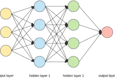
A Multi Layer Perceptron (MLP) is the simplest form of neural network. MLP or Fully Connected Networks follow a pattern where each neuron from
a layer li is connected to all the neurons in the next layer li + 1. Each connection represents a non-linear function that is generally represented by the following equation:
A=f(ωX+b)
Beingω and b the learning parameters of the neural net. ω standing for weights and b standing for bias. The number of layers and the number of neurons are hyperparameters in the model. We added MLP to our expere-ments as a neural net baseline to compare it with the different presented architectures.
Figure 3: MLP architecture example
4.3.2 Convolution Neural Networks
Convolution Neural Networks (CNN) has gained a lot of momentum since AlexNet won the imageNet competition in 2012. Since then CNN has been applied successfully in different classification tasks from human speech recog-nition to natural language processing methods.
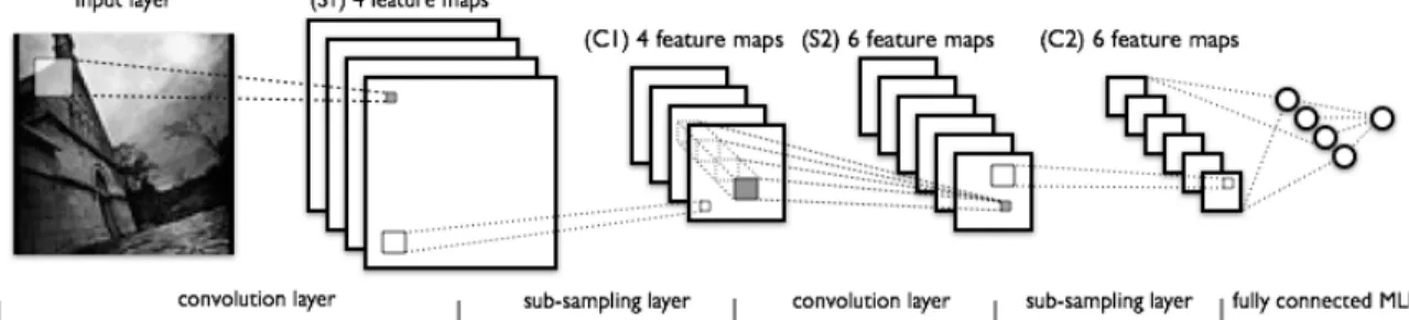
Following the classic image classification example Convolution Neural Networks work applying one filter across the input image in each layer. The intuition behind this method is that each filter can be specialized in looking for certain patterns like edges or specific changes in colors. The main dif-ference between the MLP architecture is that CNN apply the same filter to the whole input, therefore the number of learning parameters is drastically decreased. This property makes CNN easier to train and allows much deeper architectures.
CNN architectures are mostly used in image classification problems, there-fore, used with 2-D inputs. Changing the shape of the filter to 1D filters enables the CNN to be also used over times eries classification problems.
4.3.3 Fully convulutional Neural Networks
Fully Convolutional Neural Networks (FCNs) were first proposed in Wang et al. (2017) [27] for classifying univariate time series. FCN has been proven as one of the best suit architectures for this task. Fully Convolutional Neural Networks main difference with normal Convolutional Neural Networks is that they don’t use pooling layers. As a result, the series length is not reduced throughout the layers.
Keeping the full length of the time series allows deeper layers to still have more input information than traditional CNN architectures. Allowing the discovery of patterns that can be lost through the pooling phases. This architecture still uses the main idea of CNN of applying the same convolution to the whole series, sharing and therefore reducing the number of parameters to be trained.
4.3.4 Residual Neural Networks
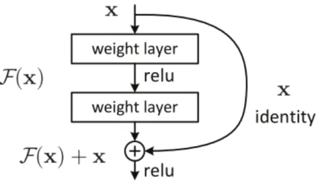
Residual net architecture was presented for the first time in 2016 by [13], as a response of the vanishing/exploding gradient problem in very deep neural systems. As shown in [24] adding layers in deep neural systems could degrade the overall performance of the system. This counterintuitive phenomenon occurs due to the inherent difficulty that non-linear layers have to represent the identity mapping. In other words, solver algorithms struggle in the task of neutralizing useless layers. Resnet architectures have solved this problem changing the desired mapping for a certain block of non-linear layers from F(x):= H(x) to F(x):= H(x) - x. Then, the original mapping is transformed to F(x)+x. The solution is equivalent but the training is simplified. This is called a shortcut (Figure 5). As an illustrative example in the uttermost case where the block is not adding any useful transformation to the input, the solver has only to set the training weights of the non-linear block to 0, letting the input pass unchanged.
Figure 5: Shortcut diagram
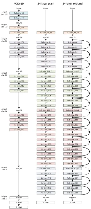
Using shortcuts repeatedly in highly deep architectures has been proven to ease the training of the nets. Figure 6 shows how the architecture of a 34 layer CNN is transformed after applying shortcuts.
5
Dataset
The dataset used in this work was created by the Massachusetts Hospital Hospital (MGH) lab. The dataset used includes 10000 sleep sessions, with an average of 7.2h per session. All the data have been acquired using a sampling frequency of 200HZ. The MGH dataset has been scored as a clinical practice by certified sleep technicians, the sleep has been classified as specified by the American Sleep of Medicine Association (AASM) guidelines.
0
1000000 2000000 3000000 4000000 5000000
N3
N2
N1
REM
W
Figure 7: Example of a classified sleep session
In Figure 7 a scored sleep session is showed. In this Figure, deeper stages (NREM3) can be seen as the parts of the session that reach the bottom part of the plot. Whereas, being awake is denoted with the line reaching the top of the plot. A sleep cycle is defined as an oscillation between NREM and REM phases of sleep. This cycle takes 1–2 hours. In Figure’s 7 session four complete cycles are achieved. Sleep phases distribution inside cycles tend
to change during a sleep session, having more deep sleep phases in the first cycles and more REM phases in the last ones.
0 250 500 750 1000 1250 1500 1750 2000 250 25 0 250 500 750 1000 1250 1500 1750 2000 250 25 0 250 500 750 1000 1250 1500 1750 2000 250 25 0 250 500 750 1000 1250 1500 1750 2000 250 25 0 250 500 750 1000 1250 1500 1750 2000 250 0 250 500 750 1000 1250 1500 1750 2000 250 25
(a) REM EEG signals
0 250 500 750 1000 1250 1500 1750 2000 1000 0 250 500 750 1000 1250 1500 1750 2000 0 100 0 250 500 750 1000 1250 1500 1750 2000 1000 0 250 500 750 1000 1250 1500 1750 2000 500 50 0 250 500 750 1000 1250 1500 1750 2000 1000 100 0 250 500 750 1000 1250 1500 1750 2000 1000 100
(b) NREM3 EEG signals
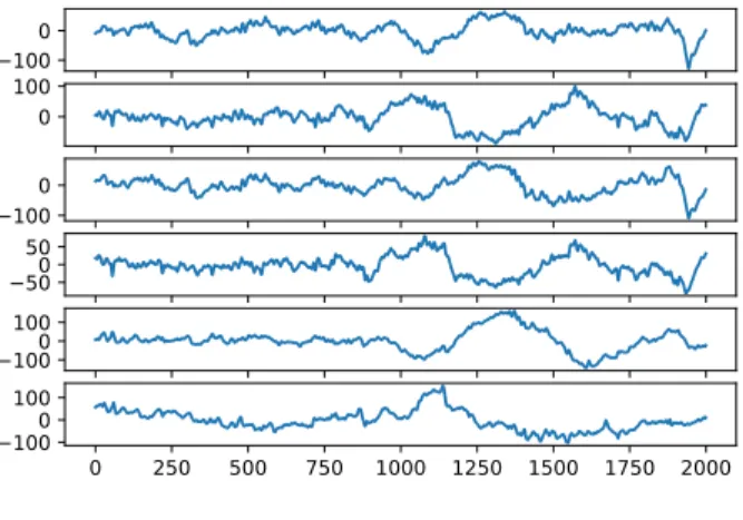
Figure 8: Example of EEG signals
0 250 500 750 1000 1250 1500 1750 2000 750 500 250 0 250 500 750 1000 1250
(a) REM ECG signals
0 250 500 750 1000 1250 1500 1750 2000 750 500 250 0 250 500 750 1000 1250
(b) NREM3 ECG signals
Figure 9: Example of ECG signals
For each sleep session EEG and ECG signals are collected (Figure 8 and 9). Sleep technicians make use of the EEG signals in order to classify the different sleep phases. Figure 8 shows a clear distinction between two EEG
waveforms. The Figure shows two examples of phases REM and NR3. REM is the sleep phase where dreaming occurs, as a result of the brain activity during this phase is intense resulting in choppy waveforms. On the other hand, NR3 being the deepest phase of sleep is the one with smoother wave-forms. ECG signals (Figure 9) are not usually used for manual scoring since there is no insight clear relation between ECG signals and phases.
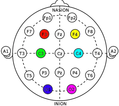
Figure 10: Electrodes layout
Figure 10 show International 10–20 system.The 10-20 system is an in-ternationally recognized method to describe and apply the location of scalp electrodes in the context of an EEG exam. In this dataset the EEG signals have been extracted using the colored set of electrodes. Ordered left to right and top to bottom. F3 being the channel 1 and O2 the channel 6.
6
Data preprocess
Following the same guidelines technicians follow to classify sleep stages, we have split the sessions in non-overlaping 30 seconds. The phase for every 30 seconds chunck has been decided using the phase mode of that chuck, that is, the most labeled phase in that period of time.
In Table 1 we can see the distribution between classes. As explained in [2] the class imbalance is a serious problem in machine learning and data mining. To overcome this problem we have manually balanced the data set to achieve the same number of samples for each class. Although balancing the data can make a slight difference between the actual size of the dataset and the new version, it does highly affects as the number of samples was relatively high. In addition, balancing the dataset was necessary for classifier training in order to avoid biased learning.
Wake REM NREM1 NREM2 NREM3
0.17 0.13 0.10 0.44 0.13 Table 1: Sleep class distribution
6.1
ECG
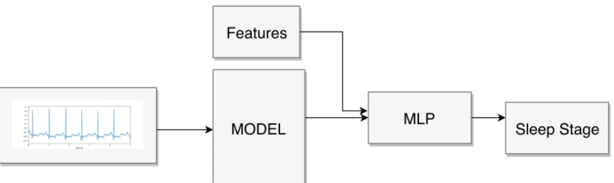
Early experiments training models against raw ECG signal had shown that models were not able to learn meaningful patterns between phases using the raw signal alone. In order to overcome this problem and ease the learning task for the models, we have decided to add some handcrafted features. We have decided to follow the standard set of time domain features set in 1996 by Malik et al. [20] extracting 8 features (table 2).
This set of features are statistic measures over intervals. An RR-interval is defined as the time in milliseconds in the RR-intervals between suc-cessive heartbeats.
Feature Definiton Formula
mRR Mean of RR intervals 1/NPn
i=1RRi
HR Mean heart rate seconds/mRR
SDNN MStandard deviation of normal–normal RR intervals q1/(N −1)Pn
i=1(RRi−mRR)2 CVRR Coefficient of variation SDN N/mRR
RMSSD Square root of the mean squared differences of successive RR intervals
q
1/(N −1)Pn−1
i=1(RRi+1−RRi)2 pNN50 Percent of normal–normal RR intervals greater
than 50 ms takes in all intervals count(RR >50)/count(RR) RRmod Mode of RR (the value repeated most often in RR) −
RRdifmod Mode of RR’s first order difference − Table 2: ECG time features
In order to add these features to the models, we have added a fully con-nected layer at the end of each architecture. This new layer is fed with the output of the model concatenated with the extracted features. This added layer has as output the probability distribution between phases. This new architecture is shown in Figure 11.
MODEL Sleep Stage Features
MLP
Figure 11: ECG structure models
6.2
EEG
Since the classification using EEG signals is an easier task we have not added any handcrafted feature to the models. Therefore, the architecture followS the usual predicting pipeline (Figure 12)
MODEL Sleep Stage
7
Experiments and results
7.1
Experimental setup
For each model, we have trained it using the 80% of the dataset, 10% as validation data and 10% as testing data. The hyperparameters of the models have been chosen empirically. In table 3 the best configurations are shown. The first column denotates the number of layers with training parameters, the second column shows the total of trainable parameters in the whole model, the third column shows the loss function used, the fourth shows the minimum
learning rate used in the training algorithm,epochs are defined as the number of times the model has iterate over the dataset,batch denotates the number of samples trained simultaneously, and algorithm the method used for training the parameters.
Model #Layers #Parameters Loss #Learning rate #Epochs #Batch Algorithm
MLP 4 3,504,005 Entropy 0.1 100 16 Adadelta
CNN 3 40,409 Entropy 0.001 100 16 Adam
FCNN 7 266,373 Entropy 0.0001 100 16 Adam
ResNet 24 504,645 Entropy 0.0001 100 16 Adam
7.2
ECG
The first classification task is between the two main classes wake and sleep. We defined wake as the wake state and sleep as the set of the others. This classification aims to be able to count the number of sleeping hours a patient sleeps during a session. The best accuracy is achieved by the residual net and the FCN models reaching a 79-80% (first row of Table 4).
KNN MLP CNN FCN RESNET
2-class 0.61 0.55 0.71 0.79 0.80
3-class 0.29 0.35 0.41 0.47 0.49
4-class 0.22 0.24 0.30 0.27 0.32
5-class 0.21 0.22 0.28 0.23 0.29
Table 4: Accuracy different models over different number of classes
Wake
REM
NREM
Predicted label
Wake
REM
NREM
True label
0.62
0.27
0.10
0.17
0.38
0.46
0.16
0.32
0.52
Normalized confusion matrix
0.2
0.3
0.4
0.5
0.6
Figure 13: 3-class resnet confusion matrix
For the 3-class classification, we have separated the classes between Wake, REM and NREM. Being NREM the group including NREM1, NREM2 and
NREM3. In this case the accuracy achieved by the best models is 47%-49%. This decreasing of accuracy is due to the difficulty to distinguish between REM and NREM phases. Figure 13 shows the confusion matrix of the resid-ual net model where REM and NREM classes are highly misclassified.
The accuracy achieved by the models for the 4-class and 5-class classifi-cation is 32% and 29%. Table 4 shows an acute decrease of accuracy for the FCN in this multi-class, whereas the CNN and the Residual net maintain a similar performance for this task.
7.3
EEG
The EEG signal has been used for classifying the sleep stages between the 5 classes. With the EEG channel signal, we have explored training against the different 6 channels individually. The accuracy achieved is shown in Table 5. The results show that the CNN architecture is the best suited for the EEG classification task reaching a 65% of accuracy. For this task, the best performance channels have been the first 4, whereas the last two have reported lesser accuracy. The last 2 channels represent the two posterior electrodes o1 and o2 (Figure 10).
KNN MLP CNN FCN RESNET EEG0 0.323 0.273 0.659 0.473 0.637 EEG1 0.453 0.606 0.629 0.606 0.542 EEG2 0.473 0.518 0.664 0.518 0.563 EEG3 0.422 0.274 0.659 0.474 0.579 EEG4 0.399 0.472 0.413 0.472 0.406 EEG5 0.455 0.463 0.602 0.463 0.368 Table 5: Accuracy obtained in the different models
Wake REM N1 N2 N3 Predicted label Wake REM N1 N2 N3 True label 0.87 0.11 0.01 0.00 0.01 0.12 0.62 0.08 0.15 0.03 0.02 0.14 0.40 0.27 0.17 0.01 0.06 0.08 0.83 0.02 0.03 0.09 0.17 0.04 0.66
Normalized confusion matrix
0.1 0.2 0.3 0.4 0.5 0.6 0.7 0.8
Figure 14 shows the confusing matrix of the best performancing model. The confusion matrix shows that the model performs best classifying the phases wake and NREM3. On the other hand, the model struggles to cor-rectly classify NREM1 phases, wrongly classifying them as mostly as N2 and N3.
8
Conclusion
In this work, we have explored the automation of sleep staging using two different signals independently EEG and ECG. To do so, we have used dif-ferent neural network architectures that had been shown to excel in the area of time series classification.
The solution using only one EEG electrode is the one that has achieved the best performance. We have done an exhaustive search across the different architectures and EEG electrodes. The best combination has been the first 4 electrodes (f3, f4 ,c3, c4) combined with the Convolution Neural Network architecture reporting a ∼65% of accuracy.
The solution using the ECG signal has explored the possibilities of classi-fying a different number of classes. The reported accuracies starting from the whole class problem and ending to a wake-sleep classification are: 29%, 32%, 49%, 80%. These results show a promising possibility of an in house sleep disorder early detector. Especially for the Wake-REM-NREM classification. Starting from the ECG signal alone having a 49% of accuracy and adding wearable devices data to the model such as accelerometers, gyroscopes, etc. A highly accurate at home classifier could be feasibly done.
References
[1] Sleep Studies: Tests & Results - National Sleep Foundation. [2] Behrouz Alizadeh Savareh, Azadeh Bashiri, Ali Behmanesh,
Gho-lam Hossein Meftahi, and Boshra Hatef. Performance comparison of machine learning techniques in sleep scoring based on wavelet features and neighboring component analysis. PeerJ, 6:e5247, 7 2018.
[3] Donald J Bemdt and James Clifford. Using Dynamic Time Warping to FindPatterns in Time Series. Technical report, 1994.
[4] David E. Blask. Melatonin, sleep disturbance and cancer risk. Sleep Medicine Reviews, 13(4):257–264, 8 2009.
[5] Daniel Bushey, Kimberly A Hughes, Giulio Tononi, and Chiara Cirelli. Sleep, aging, and lifespan in Drosophila. BMC Neuroscience, 11(1):56, 4 2010.
[6] Bj¨orn Dahl¨of. Cardiovascular Disease Risk Factors: Epidemiology and Risk Assessment. The American Journal of Cardiology, 105(1):3A–9A, 1 2010.
[7] L. Fraiwan, K. Lweesy, N. Khasawneh, M. Fraiwan, H. Wenz, and H. Dickhaus. Classification of Sleep Stages Using Multi-wavelet Time Frequency Entropy and LDA. Methods of Information in Medicine, 49(03):230–237, 1 2010.
[8] Luay Fraiwan, Khaldon Lweesy, Natheer Khasawneh, Heinrich Wenz, and Hartmut Dickhaus. Automated sleep stage identification system based on time–frequency analysis of a single EEG channel and ran-dom forest classifier. Computer Methods and Programs in Biomedicine, 108(1):10–19, 10 2012.
[9] Ary L. Goldberger, Luis A. N. Amaral, Leon Glass, Jeffrey M. Haus-dorff, Plamen Ch. Ivanov, Roger G. Mark, Joseph E. Mietus, George B. Moody, Chung-Kang Peng, and H. Eugene Stanley. PhysioBank, Phys-ioToolkit, and PhysioNet. Circulation, 101(23), 6 2000.
[10] Salih G¨une¸s, Kemal Polat, and S¸ebnem Yosunkaya. Efficient sleep stage recognition system based on EEG signal using k-means clustering based
feature weighting. Expert Systems with Applications, 37(12):7922–7928, 12 2010.
[11] Werner Haustein, June Pilcher, Joachim Klink, and Hartmut Schulz. Automatic analysis overcomes limitations of sleep stage scoring. Elec-troencephalography and Clinical Neurophysiology, 64(4):364–374, 10 1986.
[12] Kaiming He, Xiangyu Zhang, Shaoqing Ren, and Jian Sun. Delving Deep into Rectifiers: Surpassing Human-Level Performance on Ima-geNet Classification, 2015.
[13] Kaiming He, Xiangyu Zhang, Shaoqing Ren, and Jian Sun. Deep Resid-ual Learning for Image Recognition, 2016.
[14] Yoshitaka Kaneita, Takashi Ohida, Makoto Uchiyama, Shinji Takemura, Kazuo Kawahara, Eise Yokoyama, Takeo Miyake, Satoru Harano, Ken-shu Suzuki, and Toshiharu Fujita. The Relationship Between Depression and Sleep Disturbances.The Journal of Clinical Psychiatry, 67(02):196– 203, 2 2006.
[15] Andrej Karpathy, George Toderici, Sanketh Shetty, Thomas Leung, Rahul Sukthankar, and Li Fei-Fei. Large-Scale Video Classification with Convolutional Neural Networks. In2014 IEEE Conference on Computer Vision and Pattern Recognition, pages 1725–1732. IEEE, 6 2014. [16] Serkan Kiranyaz, Turker Ince, and Moncef Gabbouj. Real-Time
Patient-Specific ECG Classification by 1-D Convolutional Neural Networks.
IEEE Transactions on Biomedical Engineering, 63(3):664–675, 3 2016. [17] Alex Krizhevsky, Ilya Sutskever, and Geoffrey E. Hinton. ImageNet
classification with deep convolutional neural networks. Communications of the ACM, 60(6):84–90, 5 2017.
[18] Guillaume Lample, Miguel Ballesteros, Sandeep Subramanian, Kazuya Kawakami, and Chris Dyer. Neural Architectures for Named Entity Recognition. 3 2016.
[19] Sheng-Fu Liang, Chin-En Kuo, Yu-Han Hu, and Yu-Shian Cheng. A rule-based automatic sleep staging method. Journal of Neuroscience Methods, 205(1):169–176, 3 2012.
[20] M. Malik, J. T. Bigger, A. J. Camm, R. E. Kleiger, A. Malliani, A. J. Moss, and P. J. Schwartz. Heart rate variability: Standards of mea-surement, physiological interpretation, and clinical use. European Heart Journal, 17(3):354–381, 3 1996.
[21] E Sforza and S Vandi. Automatic Oxford-Medilog 9200 sleep staging scoring: comparison with visual analysis. Journal of clinical neurophys-iology : official publication of the American Electroencephalographic So-ciety, 13(3):227–33, 5 1996.
[22] Rakesh Kumar Sinha. Artificial Neural Network and Wavelet Based Automated Detection of Sleep Spindles, REM Sleep and Wake States.
Journal of Medical Systems, 32(4):291–299, 8 2008.
[23] Jack R Smith and Ismet Karacan. EEG sleep stage scoring by an auto-matic hybrid system. Electroencephalography and Clinical Neurophysi-ology, 31(3):231–237, 9 1971.
[24] Rupesh Kumar Srivastava, Klaus Greff, and J¨urgen Schmidhuber. Train-ing Very Deep Networks. 7 2015.
[25] Robert Stickgold. Sleep-dependent memory consolidation. Nature, 437(7063):1272–1278, 10 2005.
[26] Jen Hong Tan, Yuki Hagiwara, Winnie Pang, Ivy Lim, Shu Lih Oh, Muhammad Adam, Ru San Tan, Ming Chen, and U. Rajendra Acharya. Application of stacked convolutional and long short-term memory net-work for accurate identification of CAD ECG signals. Computers in Biology and Medicine, 94:19–26, 3 2018.
[27] Zhiguang Wang, Weizhong Yan, and Tim Oates. Time series classi-fication from scratch with deep neural networks: A strong baseline. In 2017 International Joint Conference on Neural Networks (IJCNN), pages 1578–1585. IEEE, 5 2017.