Machine Learning methods for classification of Acid Sulfate soils in Virolahti

(1)

Machine Learning methods for classification of Acid

Sulfate soils in Virolahti

Virginia Estévez Nuño

Master’s Thesis

Master of Engineering - Big Data Analytics

May 2020

(2)

MASTER’S THESIS

Arcada University of Applied Science

Degree Programme: Master of Engineering - Big Data Analytics

Identification number: 7754

Author: Virginia Estévez Nuño

Title: Machine Learning methods for classification of Acid

Sulfate soils in Virolahti

Supervisor (Arcada): Kaj-Mikael Björk

Commissioned by:

-Abstract:

Acid Sulfate (AS) soils are among the most dangerous soils naturally occurring soils. This is due to the several ecological damages that they can generate. In Europe, the highest concentration of this type of soils is located in Finland. This represents one of the major environmental problems of the country. To solve this issue it is essential the localization of the areas where these soils appear, and try to avoid their exposition to oxidizing conditions. Despite of the effort done during the last decade, there are hardly any AS soils mapping done in the country. The main reason is that the tra-ditional methods used for AS soil mapping are very laborious and take a long time. Nowadays, thanks to new technologies a large amount of data is generated in soil sci-ence. As a result, several machine learning techniques can be used for the classification of AS soils. The use of these techniques will streamline the process and improve the accuracy of the AS soils mapping. The study of this master thesis has focused on the evaluation of different machine learning techniques for the AS soils classification in a small region of Finland. The goal is to find suitable methods for this. Random forest, Gradient boosting, Support vector machine and a Convolutional neural network have been analyzed in detail. The study area corresponds to Virolahti, which is located in the south-east of Finland. Two different datasets have been created, one for the case of deep learning and another for the rest of the methods. The results show that gradient boosting and random forest are very good methods for the classification of AS soils, whereas support vector machine is not very good. The convolutional neural network gives poor results, may be due to the small size of the dataset created.

Keywords: Acid sulfate soils, machine learning, deep learning

Number of pages: 55

Language: English

(3)

1 INTRODUCTION

The study done in this master thesis combines two main research fields, soils science and artificial intelligence. Specifically, the classification of acid sulfate soils using different machine learning techniques is done for a small area of Finland.

1.1 Acid Sulfate Soils

Nowadays, the soil science is fundamental for the development of different fields that di-rectly affect the society and economy, such as natural resources, energy, agriculture, cli-mate change or the construction of infrastructures. The soil science studies and analyzes the soils in a natural environment. One of the type of soils that attracts more attention are the acid sulfate (AS) soils, which can generate several ecological damages. From an environmental point of view, the AS soils are considered the most problematic. This type of soils appears in coastal regions and also in freshwater wetlands around the world, with major occurrences in Australia, Africa, Asia and Latin America (Ritsema et al. (2005)). In Europe, the highest concentration of AS soils is found in Finland, about 1600-3000 km2 located on the Finnish coastal areas (Edén et al. (2012a), Yli-Halla (1997), Fäaltmarsch et al. (2008 )), see Fig. 1. This leads to one of the major environmental problems of the country.

(8)

In Finland the AS soils were formed at the sea bottom of the Baltic Sea during the Holocene. Their creation occurred in the absence of oxygen. After the glaciation the land has raised up, and at present these soils are above the sea level. This represents a serious problem due to AS soils have a high concentration of metal sulfides that oxidize under aerobic conditions, leading to the formation of sulfuric acid. As a result, acidifica-tion of the soils and metal polluacidifica-tion take place.

Among the main problems generated by the AS soils there are the production of metals and acidification of the soils, which have a high impact on the flora and fauna. Partic-ularly dangerous is the large amount of metals that ends in the rivers and watercourses. This quantity is much larger (between 10 and 100 times) than the one derived from the whole Finnish industry (Fäaltmarsch et al. (2008 ), Sundström et al., (2002)). The large concentration of metals and the acidification of watercourses, strongly affect the biodiver-sity of fish and other aquatic organisms. However, one of the most alarming consequences of the acidification of the watercourses is the large-scale fish kills that have taken place in Finland during years. The first one that is known occurred in 1834, but there were also large-scale fish kills in 1969-1971, 1996 and more recently in 2005-2006. This not only supposes a great environmental disaster, but also it can have devastating consequences in the economy.

The agriculture and its productivity are also strongly affected by the AS soils. There is one study where it is shown that some crop plants from areas with this type of soils have high concentration of some metals (Palko (1986)). Moreover, it has also been found higher concentration of metals in the cow milk from farms located in AS soil areas (Alhonen et al., (2006)). On the other hand, entire crops may fail due to the acidity of the soil, which would lead to significant economic losses.

From the point of view of health there are not conclusive studies, although there is a discussion about the influence of the AS soils in the development of some illness such as Parkinson and Alzheimer (Amaducci et al., (1986), Zatta et al., (2003), Brown et al., (2005)). Furthermore, it would be interesting to know how the health is affected by the consumption of products with a high concentration of metals.

(9)

order to plan new infrastructures such as a bridge, a road or a building, it is essential to know the types of soils. AS soils can contribute to the corrosion of steel infrastructures or in the fast deterioration of a building, which can have a significant economic impact.

1.2 Artificial Intelligence

Artificial intelligence (AI) is an emerging research field with a great potential to analyze and solve problems in different fields such as sciences, medicine, business, security or industry. Moreover, it is completely integrated in our every-day-life. One of the most important areas in AI is the Machine learning (ML), where thanks to algorithms the com-puters can learn from data. At present, the society is generating a large quantity of data that can be used for studying different research fields. As a result, ML is becoming a science with a large impact on society and economy.

1.3 Motivation and Aim of the Study

As we have already seen, the AS soils are a serious problem for the country from an eco-logical, social and economic points of view. In order to minimize the damage generated by this type of soils, it is fundamental to localize them and try to avoid their exposition to oxidizing conditions. Thus, the first step to reduce the damages is the creation of AS soils maps. Although various efforts are being made towards this goal, there are barely AS maps. In general, AS soils mapping in Finland has been made by traditional methods, with soil sampling and measurements of soil-pH (Palko (1994)). However, these methods are very laborious and take a long time.

Nowadays, thanks to the new technologies a great quantity of data is generated in soil science. This allows that several methods of machine learning can be used for predicting and classifying soil maps (McBratney et al., (2003)). As a result of the use of these methods, the process of AS soil mapping will be faster and more efficient. Furthermore, AS mapping with a larger precision will have a great impact on the mitigation of the ecological damages generated by this type of soils.

The motivation of this master thesis is to speed up the AS mapping as well as to improve its accuracy using artificial intelligence. The main goal of this work is to find methods that are able to classify the AS soils correctly. For this, the research has focused on the

(10)

evaluation of different machine learning techniques in the classification and prediction of AS soils in a region of Finland.

1.4 Overview

Before starting with the study done in this master thesis, we will review the previous works in digital soil mapping (DSM), and specifically in the case of acid sulfate (AS) soils. This will allow us to know what has already been done on the research field.

A soil map is a graphic representation of the spatial distribution of the soils classes or attributes for a given area. The idea of relating the geographical coordinates and soil types was developed in 19th century by Dokuchaev (1883), and was the principle of soil science. Furthermore, he was also pioneer in the analysis of the properties of the soils by cutting and digging in the ground. These field samples are known as point observations and are very important for the preparation of DSM. The first soil map created taking into account the point observations was done in 1883 by Dokuchaev, and is a map of the humus content in Russia. In addition to the methods, other important conclusion from this work is that the soils depend on several factors.

In the early 1990s, computers and numerical models began to be used in the development of soil maps, leading to the digitization of the soil maps (DSM) (Minasny and McBratney (2016)). At the same time, studies based on geographic information systems (GIS) data appeared (Skidmore et al., (1991), Bell et al., (1992), Odeh et al., (1992a), Moore et al., (1993), McKenzie and Austin (1993)). All this meant a great progress in soil mapping, leading to the improvement of the accuracy of the new maps (Bazaglia et al., (2013)). However, at present there is a lack of DSM in the world (McBratney et al., (2003)). This is because of the traditional methods used in their creation are very expensive and slow. Due to the importance of DSM in the treatment of different areas that directly affect the economy and society, it is necessary to develop new techniques in the research field.

The general method to create a DSM is thescor pan model (McBratney et al., (2003)), which is based on previous Jenny’s equation (Jenny (1941)) and the ideas of Dokuchaev (Dokuchaev (1883)). Thescor pan model is used for predicting or classifying the soils through several factors:

(11)

S= f(s,c,o,r,p,a,n) (1)

where S is the soil class or attribute to predict, and the scor pan factors: (s) soil; (c)

climate;(o)organisms, vegetation, fauna or human activity;(r)topography or relief and landscape attributes;(p)parent material and lithology;(a)age, time factor; and(n)space, spatial position. For connectingSto thescor panfactors we use an empirical quantitative function, f. In other words, f represents the method that will be used in the prediction or classification. This method can be any machine learning model such as a decision tree (DT) or artificial neural network (ANN), and will depend on the type of data. To predict or classify soils it is not necessary to include allscor pan factors in the model. So far, most of the works (around the 80%) have used one or two factors, although there are also studies with three and four. For prediction and classification in DSM the factors most used arer(80%) ands(35%). Their combination is also the most frequent. Inside the relief or topographic factor(r), the digital elevation model (DEM) and the data derived from this are the most used. The rest of the factors have also been taken into account although to a smaller extent, o (25%), p (25%), n (25%) and c(5%) (McBratney et al., (2003)). This give us an idea about the kind of data needed to create a DSM.

On the other hand, choosing a machine learning technique to predict soil attributes or classify soils is not easy. This will depend on several factors such as the dataset or the study to be carried out. In general, supervised methods are used for the classification of soil classes, whereas the soil attributes are predicted by regression models. So far, several methods of machine learning have been used in DSM. Most typical are neural networks, fuzzy logic, linear models or random forest. Linear models (LM) were of the first methods used for the digital mapping of soil attributes (McKenzie and Austin (1993), Odeh et al., (1995), McKenzie and Ryan (1999), Park and Vlek (2002)) and soils classes (Gessler et al., (1995), Campling et al., (2002)). Decision trees (DT) were also very popular in the prediction of the properties of the soils (Breiman et al., (1984), Shatar et al., (1999), Pachepsky et al., (2001), McKenzie and Ryan (1999)) and classification (Breiman et al., (1984), Lagacherie and Holmes (1997), Bui et al., (2003)). The main problem of DT is the overfitting of the training data, which leads to high error in the prediction. Fuzzy logic (FL)(Zadeh (1965)) is other machine learning method frequently used in soil mapping

(12)

(Zhu et al., (1996), Zhu et al., (2001), Beucher et al., (2014)).

During last decade, random forest (RF) and artificial neural network (ANN) have become in the most used methods in DSM. Random forest is a technique where the prediction of different decision trees are taken into account. Unlike the case of a DT, RF corrects the overfitting, giving good results. RF has been used for predicting soil properties (Grimm et al., (2008), Behrens et al., (2010), Schmidt et al., (2004)) and soil classes (Gambill et al., (2016), Teng et al., (2018)). On the other hand, an artificial neural network is a data-driven method very good in the recognition and classification of data. Fig. 2 shows the typical structure of an ANN, which consists of input, hidden and output layers. The func-tion of the hidden layers is to obtain useful informafunc-tion from input layers to predict the outputs. Currently, ANNs are widely used for soil mapping in both cases, for predicting soil properties (Chang and Islam, (2000), Misnany and McBratney (2002), Lentzsch et al., (2005), Viscarra Rossel and Behrens (2010)) and soil classes (Zhu (2000), Behrens et al., (2005), Boruvka et al., (2006), Cavazzi et al., (2013), Chagas et al., (2013), Silverira et al., (2013), Beucher et al., (2013, 2015, 2017)).

Inputs Hidden Layer

Outputs

weights

Figure 2. Sketch of an artificial neural network

Recently, a new technique is used in soil science, Deep learning (DL) (LeCun et al., (2015), Schmidthuber (2015)). Typically, DL is used in object detection, image recog-nition or semantic segmentation (LeCun et al., (1990), LeCun and Bengio, (1995)). This method is based on neural networks and is ideal to treat and classify large quantity of

(13)

images. DL has been used in DSM for predicting soil moisture (Song et al., (2016)) and soil carbon (Padarian et al., (2019), Wadoux et al., (2019)), and in the multi-scale terrain feature construction (Behrens et al., (2018)).

This master thesis is focused on the acid sulfate soil mapping. In Finland, AS soils have been widely studied (Palko (1994), Triipponen (1997), Yli-Halla (1997), Österholm et al., (2004), Roos and Åström (2005), Edén et al. (2012a), Edén et al., (2012b), Toivonen et al., (2013), Beucher et al., (2013, 2014, 2015)). Since 2009, the Geological Survey of Fin-land (GTK) is working on the creation of an AS map for the whole country. For this, they are focused on the field work to obtain point observations of the coastal area of Finland. Despite of the effort, there are hardly AS soils maps, and the most of them correspond to very small areas. The first two AS maps have been done using traditional methods (Palko (1994), Triipponen (1997)). Some works of AS soils classification have been done with machine learning methods, fuzzy logic (Beucher et al., (2014)) and ANN (Beucher et al., (2013, 2015)). The two works done with an ANN have used the same dataset but different ANN. In the first work (Beucher et al., (2013)) it is considered a Radial Basis Functional Link Nets (RBFLN) (Looney (2002)). Whereas in the second (Beucher et al., (2015)) the ANN is based on Radial Basis Function (RBF), using a package called RSNNS (R Stuttgart Neural Network Simulator (Bergmeir et al., (2012)). Both methods are good in the prediction and classification of AS soils, and better than fuzzy logic method (Beucher et al., (2014)). Contrary to Neural Networks methods, which require a large number of known sites to carry out the prediction or classification of the problem, Fuzzy logic is relevant to predict soil properties in areas where the statistical analysis is not possible due to there are not enough number of known sites. Although FL is a good method for recognition studies of large areas, produces maps with very low precision.

1.5 Research questions

As we have seen in the previous section, several machine learning techniques have been used in the AS soils mapping. However, there are many methods that have not been used that could be more appropriate for this purpose. The use of more adequate techniques would lead to better results in the classification, and as a consequence a larger accuracy in the AS soils mapping. Thus, the main research questions of this master thesis are:

(14)

1. Can other machine learning techniques classify the AS soils?

2. How suitable are these new methods in the classification of AS soils?

In order to answer these questions, the research is focused on the study of new machine learning techniques for the AS soils mapping. The objective is to find methods that are able to classify AS soils correctly.

In this work, I have analyzed four different machine learning methods for AS soil mapping in a small area of Finland. The methods are random forest, gradient boosting, support vec-tor machine and convolutional neural network. Except for the random forest, the rest of these machine learning techniques have never been applied to the AS soils classification. However, it is expected to obtain good results with some of them. Thus, these methods will be evaluated to determine their suitability for the classification and prediction of AS soils.

On the other hand, the dataset plays a fundamental role in the classification. A good characterization of the soils as well as their classification will depend on the type of data orscor panfactors used in the study. Then, the third research question is:

3. What are the most appropriate data for the AS soils classification? And for the different methods?

For this, I have created two different datasets. One for the deep learning technique, which is an image dataset, and another for the rest of the methods.

1.6 Structure of the thesis

In addition to the introduction, this master thesis consists of four more chapters. In the next chapter I provide a complete description of the dataset created and used in this work. The different machine learning techniques analyzed in this research will be explained in the third chapter. Moreover, in this chapter a detailed explanation of the creation of the dataset required for the convolutional neural network is given. In the fourth chapter the results obtained by the different methods and their comparison are presented. Last chapter is dedicated to the conclusions of this research work.

(15)

2 DATASET

The area chosen for the study of AS soil classification is Virolahti, located in the south-east of Finland, see Fig. 3. So far, no AS soil mapping has been made in this area. For the creation of DSM, different types of spatial data can be used to predict or classify soil types or properties. Discrete sampling data or remote sensing data such as LiDAR, geophysics or satellite imagery are some of them. For the study done in this master thesis, the dataset consists of two different types of spatial data, the point observations and the covariate layers.

Figure 3. Location of the study area, Virolahti.

2.1 Point Observations

The point observations (PO) correspond to soil samples taken in the field by the geologist. These discrete sampling data will play a fundamental role in the training of the models. Geological survey of Finland (GTK) has provided me these data. Table 1 shows some PO from Virolahti. For each point the spatial coordinates, the minimum values of pH in the field and in incubation in the lab, the sulfur, as well as if the PO is AS soil or not are given. The criteria for the classification of the AS soils depends on different factors. In Finland the classification criteria for AS soils has been modified recently (Boman et al., (2020)). The PO used in this master thesis are already classified with the new criteria.

(16)

xcoord ycoord min-field-pH min-incub-pH max-tot-Sulfur AS soil

1 523859.06 6721235.76 6.6 5.0 363.0 0

2 507640.17 6714843.53 5.9 3.5 2000.0 1

3 527194.76 6710768.22 3.7 3.0 5950.0 1

4 528664.05 6724960.91 6.5 5.3 955.0 0

Table 1. Point Observations from Virolahti area.

2.2 Covariates layers

The environmental covariate layers are a raster dataset generally obtained from remote sensing data. As this region has never been analyzed, I have created the covariate layers using Qgis. A total of sixteen covariate layers of three different types: terrain, geophysics and quaternary. All of them with the same resolution or grid size (50x50)m. As I am working with spatial data it is very important that all covariate layers have the same coor-dinate reference system (crs), which is ETRS89/TM35FIN(E,N) in Finland. The PO have the same crs.

2.2.1 Terrain

The terrain or relief layers are derived from the digital elevation model (DEM), which is obtained from LiDAR elevation maps. LiDAR is based on laser scanning and has very high resolution. For the calculation of the DEM, I have obtained the data from National Land Survey of Finland (NLS). Fig. 4 shows the DEM of the Virolahti area.

(17)

The terrain layers calculated for the raster dataset are: DEM, slope, aspect, hillshade, roughness, profile curvature, tangential curvature, valley depth, topographic wetness in-dex (TWI), topographic position inin-dex (TPI), topographic ruggedness inin-dex (TRI), and catchment area. In Fig. 5 some of them are represented. There are terrain layers directly derived from the DEM such as slope or aspect. However, there are other layers that for their calculation other intermediate layers have to be created. This is the case of topo-graphic wetness index (TWI) where other 3 layers are needed.

(a) (b)

(c) (d)

Slope Aspect

Hillshade TWI

Figure 5. Terrain layers derived from DEM. a) Slope. b) Aspect. c) Hillshade. d) TWI.

2.2.2 Quaternary geology

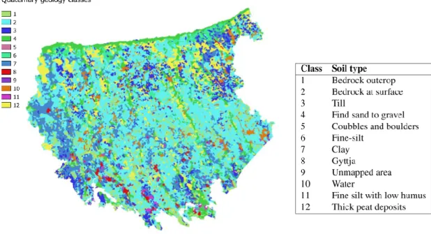
The Quaternary geology map is composed of 12 different classes of soils or materials, see Fig. 6. The soil types for the quaternary geology map can be also seen in the figure.

2.2.3 Geophysics

The geophysics data where magnetism or electric conductivity are taken into account can give important information about the types of soils. For example, the high quantity of sulfur presented in AS soils seems to be reflected in geophysics. The necessary data for the calculation of the geophysics layers has been provided by GTK. I have created three layers: electromagnetic real and imaginary components, and the resistivity.

(18)

Figure 6. Quaternary geology layer.

where it is represented the electromagnetic imaginary component above the quaternary layer. For the study, all the covariate layers have to have the same contour. This will be very important for the prediction. For this reason I have clipped all the covariate layers with the contour of the geophysics layers. This has given me a lot of problems, although after several calculations I have managed to create a vector layer with the desired area. Thanks to this layer I have clipped the raster layers correctly.

With the change of contour, the size of the layers has been slightly reduced and some point observations have been left out of the new study area. As a consequence, the dataset is reduced to 316 PO, 209 Non-AS and 105 AS soils.

2.3 Relation between Point Observations and Covariates

layers

For the AS soil classification it is necessary to relate the PO and the environmental co-variate layers. This will give us information about the characteristic values of a coco-variate layer for both classes of soils. Then, for this work the relevant information from the PO are the spatial coordinates and the soil type, i.e. if the point is AS soil or not. In Fig. 8, PO and DEM layer are represented for the whole area of Virolahti. As it can be observed,

(19)

Figure 7. Electromagnetic imaginary component layer above the quaternary layer. The size of the geo-physics layer is smaller.

all points are located at the bottom of the layer. This leads me to wonder if a correct classification or prediction can be made for the whole area with these PO. To be able to answer this question it is required to do statistics.

2.3.1 Statistics

In order to determine if the PO are representative for the whole area I have done the statistics for all PO and compared with the values of the whole covariate layers. The comparison can be seen in Table 2, where there are the values for three different layers, DEM, slope and electromagnetic real component. As it can be observed, the range of values of the PO is much smaller than the range of values for the whole area. This is clearly seen for the maximum value in all the cases analyzed. However, only with these statistics values it is extremely difficult to determine if the points are representative of the most regions of the layer. Note that one point can have a maximum or minimum value, whereas most of the points could be in a range quite similar to the one of the PO.

On the other hand, it is important to highlight that the PO with the maximum value for DEM is 38.89. This means that all PO are located below 40 m above the sea level. Since the formation of the AS soils, the land has uplift an average of 4 mm per year. As a result, it is expected to find AS soils in areas with an elevation below 40 and 50 m, but not above

(20)

Non AS soils AS soils -0.7 117.9

Figure 8. Point Observations and DEM for Virolahti.

DEM Slope AEM real

W. area PO W. area PO W. area PO

Max 117.900 38.890 61.516 15.061 15894.864 14867.694

Mean 47.271 14.597 4.397 2.440 249.856 259.820

Min -0.700 0.211 0 0.073 -2658.248 -845.814

Std 23.911 9.197 4.713 2.522 1211.356 1053.270

Table 2. Comparison between the statistics of some covariate layers for the whole area of Virolahti (W.area) and the point observations (PO). The covariate layers are DEM, slope and electromagnetism real compo-nent (AEM real).

this. Probably the elevation be larger than this in the most of the regions of the upper area of Virolahti, and for that reason the geologists have not analyzed points in this area. This and the fact that I do not have points in the upper area to validate the results obtained by the machine learning methods, have led me to reduce the study area to the lower half region where the PO are located.

(21)

3 RESEARCH METHODOLOGY

The study done in this master thesis is the AS soils classification in Virolahti. This is a binary classification problem, where the two classes are AS and Non-AS soils. Nowadays, there are different machine learning techniques for doing a binary classification. The most appropriate method will depend on the type of data. In this work I have analyzed several methods.

As we already saw in the previous chapter, my dataset consists of point observations (PO) and covariate layers, which are spatial data. Depending on the relation between the PO and the covariate layers, I divide the methods in two types, conventional and deep learning. In the conventional methods, the information from the covariates layers is the related to the PO. This means that each PO will have associated values of the covariate layers considered in the study. On the other hand, the information about the surroundings of the PO can also be taken into account. This can be done with deep learning techniques. In this master thesis, the deep learning technique used is a Convolutional neural network. For this method, the data need a new preprocessing. At the end of this chapter I will explain how I have prepared the data for this method.

In soil science the most used methods for classification and prediction are the conven-tional. So far, the deep learning techniques have been barely used. In order to find the most suitable method for AS soils classification, four different methods have been ana-lyzed in this master thesis. Random forest, Gradient boosting, Support vector machine and a Convolutional neural network (CNN). This last technique has been recently used in the prediction of soil carbon with good results (Padarian et al., (2019)). On the other hand, Random forest have been widely used for the prediction and classification of the soils.

3.1 Random Forest

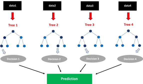
The combination of multiple machine learning techniques to create one more powerful is known as ensemble method. Random forest (RF) is one of the most used ensemble methods. RF is a supervised machine learning technique based on decision trees. This method generates different decision trees on data randomly selected, see Fig. 9 where a sketch of a RF is represented. Depending on whether the problem is a classification or

(22)

a regression, the prediction will be calculated in different way. In the case of classifica-tion, the predictions of all trees are compared and the best one is selected. Whereas for regression, the final prediction is an average of the predictions obtained from all the trees. Thanks to the trees created on random subsets of data, this method reduces the typical overfitting of the decision trees. Due to its effectiveness and precision, RF is a machine learning method widely used for classification and regression problems. Furthermore, it is a quite fast technique for not very large datasets.

data1 data2 data3 data4

Tree 1 Tree 2 Tree 3 Tree 4

Decision 1 Decision 2 Decision 3 Decision 4

Prediction

Figure 9. Sketch of a Random Forest.

RF is also very good measuring the importance of the features in the prediction or classi-fication. This is extremely useful in the case of soils classification where the features are covariate layers as the study done in this master thesis. Some works have shown that not all environmental covariates are relevant in a specific study. Moreover, these irrelevant co-variates can hindering the prediction in some cases (Ribeiro Campos et al. (2018)).

3.2 Gradient Boosting Machines

Other ensemble method based on decision trees is the Gradient Boosting Machines or Gradient Boosted Decision Trees. Unlike random forest, the gradient boosting creates the trees serially, trying to improve the prediction of the last tree taken into account the previous one. For this, each tree tries to minimize the errors in the prediction of the previous one. As a result, the overall prediction improves.

(23)

This method is used in classification and regression problems. Thanks to its accuracy and prediction speed, the gradient boosting is one of the most powerful machine learning technique for predictive studies. In general, this method is ideal for the case of large and complex data.

A weakness of this method is its sensitivity to the parameter settings. In this sense, random forest is more robust than gradient boosting.

3.3 Support Vector Machines

The Support vector machine (SVM) is a supervised machine learning technique used for problems of classification and regression. This method is widely used for binary classification. Unlike the two previous methods, it is a linear model. In the case of a classification, the model tries to divide the classes by a line, a plane or a hyperplane. For the classification I have compared the support vector classification (SVC) and their implementation Linear SVC. The difference between both is that the kernel in the Linear SVC is always linear. Among the good things of the linear models is that they are quite fast to train and predict. Furthermore, for large dataset it works very well.

3.4 Convolutional Neural Network

Deep learning is a machine learning technique. Nowadays, the deep learning and specially the convolutional neural networks (CNN) have generated great interest due to their excel-lent results in some problems such as image and speech recognition. This method learns from the representation of data through several layers which are simple transformations of the data.

One of the main problems of deep learning techniques is the large amount of data nec-essary to train the model and, thus, be efficient. A small dataset can lead to overfitting. Furthermore, in a CNN it is complicated to adjust the parameters for doing a good predic-tion or classificapredic-tion. On the other hand, in the case of soils sciences it is quite difficult the interpretation of the results.

In this work I have analyzed how the CNN method is able to classify the AS soils using image classification. For this I have had to create an image set based on my original

(24)

dataset. The preparation of the image set is explained below.

3.4.1 Data preparation

In a CNN the input layer are images. For doing the binary classification images of the both classes, AS and Non-AS soils, are needed. As it was already mentioned, the covariate layers are rasters, i.e. images of pixels. Thus, the covariate layers can be used as input layers. The problem is that each covariate layer has information for both classes, see Fig. 8. For the CNN each input image only has to have information of one of the classes. For this reason I have created the corresponding image dataset. The new images are centred at the point observations (PO), which determines the class of the image. On the other hand, the image size is conditioned by the minimum distance between two points of different class.

Calculating the distance between the PO, I have noted that there were pixels with two points. In the case of conventional methods where only the information of the covariates layers is associated to the PO, this is not a problem because both points have different information although quite similar. However, for the case of CNN this is a problem be-cause two equal images will be generated. Note that the center of the image is the pixel where the PO is located. For this reason and as in all the cases the two points were of the same class, one of the points of the pixels have been randomly removed. In total, twenty points have been eliminated from the dataset, eight for AS soils and twelve for Non-AS soils.

The minimum distance between two points of different class allows a maximum image size of 9x9 pixels, or 450x450 m. There are four pairs of points that are closer, but as all of them are of the same class, it does not matter if there is a small overlap in some pixels of the images. In a previous work for soil carbon prediction, it has been shown that the effect of the image size on the prediction appears in cases with a size above 1100x1100 m, (Padarian et al., (2019)). Moreover, for their case it was found that the range of useful information was between 300 and 900 m. Thus, I can consider that images with a size equal to 9x9 pixels are good for my study.

On the other hand, there are PO just on the border of the covariate layers. This means that the images cannot be created around these PO because the image would have pixels

(25)

without any information. One solution could be to use padding and include them in the modelling. However, I do not know if this is completely correct. In order to avoid errors I have excluded them from the dataset. Once all the problematic PO have been eliminated, the dataset consists of 187 Non-AS soils and 93 AS soils.

For the study, I have created a balanced dataset. This means equal number of samples for AS and Non-AS soils in the training set. This is very important for a correct classification and prediction of both classes. Previously, I have compared two datasets, one unbalanced and other balanced. The unbalanced contains all points of the original dataset (209 Non-AS and 105 Non-AS soils), whereas the balanced 105 for each class. The PO for Non-Non-AS soils in the balanced case have been randomly selected. The study have been done using random forest and considering 75% of the data for training and the 25% for validation. Although the accuracy for the validation set is better for the unbalanced case (79%), the precision for one of the classes is very bad compared with the other (84% for Non-AS soils and 62 % for AS soils). On the contrary, in the balanced case the precision for both classes is quite similar, (69% for Non-AS and 72% for AS) although the accuracy drops to 70%. For the AS soils classification it is very important to be able to predict both classes with a similar probability. For this reason a balanced dataset is used in the study. The importance of having identical number of PO for both classes was previously analyzed (Porwal et al., (2003)).

The balanced dataset created for the study consists of 186 PO, 93 for each class. As previously, the PO that are Non-AS soils have been randomly selected. For the model, the data have been split in an 80% for the training set and a 20% for the validation. The proportion of AS and Non-AS soils in the training set is the same. This balanced dataset has been used for all machine learning methods analyzed in this master thesis. This allows the comparison of the methods.

In the case of CNN, the image dataset has been created using the same points for the training and validation. For each PO there are n images corresponding to the different covariates layers considered in the study. The contribution of the covariate layers is the same in the training set. This means that for a given class the number of images for each covariate layer is equal. In this way the model will learn better than if the proportion is

(26)

different.

3.4.2 Model

Convolutional input 9x9 7x7 pool 3x3 AS soil Fully connected Output

Figure 10. Architecture for a convolutional neural network.

For the model I have used Keras and TensorFlow. Keras is a library which allows the creation of models for deep learning and CNN. The model is formed by several layers that transform the data in order to obtain information, and at the end be able to give a prediction. Fig. 10 shows an example of the network architecture for a standard model. The input layer is a 9x9 image that corresponds to an AS soil from my dataset. The in-formation of this input layer will be transformed through a series of layers. The first layer is one of the most important in the model, the convolutional. Through two-dimensional filters, this layer detects and extracts specific characteristics of the image. In Fig. 10 it can be seen how the input image is filtered with a 3x3 filter, leading to 7x7 images. These resulting images are the features maps. The convolutional layer is followed by an acti-vation function, which gives a non-linear behaviour to the network. Different functions such as ReLU, sigmoid or tanh can be used as activation function. After a convolutional layer I have used ReLU (Rectified linear unit), see Fig. 11. This activation function is one of the most used with the hidden layers in a CNN. The next layer applied in the model represented in Fig. 10 is a pooling layer, which reduces the feature maps generated by the convolutional layer by means of a filter. In the case of the example shown in Fig. 10, the pooling reduces the images to the half. There are two main types of pooling, max

(27)

pooling and average pooling. Whereas the max pooling takes the maximum value inside the region cover by the filter, in the case of average pooling it is considered the average of the values.

ReLU Sigmoid

Figure 11. Activation functions, ReLU and Sigmoid.

All the layers described until now correspond to the hidden layers. Convolutional and pooling layers can be applied several times on the model, which will lead to a deeper learning. In my case the images are so small that only few layers are possible in the architecture of the model as it will be seen later.

For doing the classification, all the information extracted from the hidden layers has to be converted in a one-dimensional array. This process is known as flattening. The feature vector generated will allow the connection to the fully connected or Dense layer. Among other things, this dense layer will allow to get the number of classes. Finally, an activation function to obtain the probability of the different classes has to be applied. As my problem is a binary classification, the most suitable function is sigmoid. As it can be seen in the Fig. 11, the values of this function are between 0 and 1. Thus, this function will define the behaviour of the probability in the binary case.

As it was already mentioned, a CNN needs a large amount of data to work better. A small dataset as in my case can generate overfitting. This problem can be solved with data augmentation or including dropout layers.

(28)

Data Augmentation

Data augmentation is a technique used to generate artificially more data in the training set. This will improve the ability of the model to learn and be able to predict. The new images are created from the original ones by means of different transformations such as zoom, rotation, flip or shift. Depending on the data some transformations will be more suitable than others. In Keras the data augmentation can be done via the ImageDataGenerator when the code is executed. In this way it is not necessary to save the images, which helps to solve memory problems in the case of large dataset.

In the case of my spatial data most of the transformations cannot be applied due to they will introduce noise. The most convenient is to rotate the image 90, 180 and 270 degrees. This will not only not introduce noise in the model, but will quadruple the number of images. This should be implemented in the code because ImageDataGenerator is not able to do. The rotation given by this tool takes randomly an angle between 0 and the chosen angle of rotation. For example, if the angle is 90 degrees the images will be rotated with any angle in the range [0-90] generating a lot of noise.

Dropout Regulation

Dropout is a technique to reduce the overfitting (Srivastava et al., (2014)). This con-sists of ignoring some of the input units and their connections during the training of the model. The input units not considered are randomly selected. I have used several layers of dropout in my model.

(29)

4 RESULTS

All the results presented in this master thesis have been obtained using the same PO. For the conventional methods the points have been associated with the values of the covariate layers, whereas the images for deep learning have been created from the covariate layers for these PO.

In general, machine learning techniques give better results when there are more data. However, in the case in which the data are environmental covariates this is not always true. Depending on the study a covariate layer can contribute or not. Moreover, in some cases their contribution can be negative, making the prediction worse (Ribeiro Campos et al. (2018)). For this reason, it is important to analyze the contribution of the covariates in the prediction or classification. On the other hand, the importance of a covariate will depend on the method used.

Five different covariates layers have been considered for the study of AS soils classifica-tion in Virolahti area. In Finland, previous works have considered four covariate layers (Beucher et al., (2013, 2014, 2015)): slope, real and imaginary components of geophysics and the quaternary geology. In addition to these layers I have included the digital elevation model (DEM) in the study.

Next, we will see the results obtained with the different machine learning techniques used in this work. Although first, the different metrics used to evaluate the results and the methods will be explained.

4.1 Metrics

Thanks to the metrics it is possible to know if a method is suitable for a given study or a dataset. There are different metrics for the evaluation of the machine learning methods. Here, the different types for classification problems are shown (Powers (2011)).

Accuracy

One of the most common metric is the accuracy, which is given by the number of correct predictions divided by the total number of predictions. In machine learning methods it is normal to compare the accuracy of the training set with the one of the test set. This is very

(30)

useful to know if the model has overfitting or underfitting. However, the accuracy does not give any information about how a certain class is predicted or classified. Thus, in the case of a binary classification other metrics are needed to get this information.

Confusion matrix

The confusion matrix is a typical method to evaluate a binary classification. In a confusion matrix the predicted values for both classes are represented against the actual values of the classes. Fig. 12 shows a confusion matrix, where TP is the true positives, FP the false positives, FN the false negatives, and TN the true negatives. As in a binary classification there are two classes, one is considered positive and the other negative. TP and TN are the number of items that have been correctly classified for each class. Whereas FP and FN correspond to the number of elements incorrectly classified. Unlike to the accuracy, the confusion matrix allows to visualize how the model is predicting both classes.

TP

FN

FP

TN

Predicted Values

Act

ual

V

alues

Confusion matrix

Figure 12. Confusion matrix.

Precision

The precision indicates the percentage of the samples correctly classified for a given class with respect to the total number of elements classified for that class, as it can be seen in the next equation:

(31)

precision= T P

T P+FP (2)

Recall

The recall metric is also called sensitivity. This measures the number of items correctly classified for a given class in comparison with the total number of samples for this class. The recall equation for the positive class is given by:

recall= T P

T P+FN (3)

F1-score

The F1-score also known as F score or F measure is a combination between precision and recall. F1−score=2 precision∗recall precision+recall (4) ROC curve

The ROC (Receiver Operating Characteristics) curve is one of the most important metrics for the evaluation of a binary classification model. The ROC curve represents the true positive rate (TPR) as a function of the false positive rate (FPR). Thanks to the area under the curve (AUC), it is possible to know if the model is a good classifier or not. In the case where the value of AUC is close to one, the model is good in the classification of the classes. As the value of the area decreases, the ability of the model to classify the classes will also do. For an AUC equal to 0.5, the model is not able to distinguish between both classes. This case corresponds to a random classifier. An AUC value below 0.5 means a bad classifier.

(32)

4.2 Random Forest

The first machine learning technique that I have analyzed is Random Forest, which is one of the most used methods in soil science.

For the evaluation of the model it is important the selection of the parameters. Depending on the values of the parameters of a model, it can give good or bad results for the same dataset. For all conventional methods I have used grid search, which is a method that adjusts the parameters of the model to obtain the best performance.

13

6

5

14

Non-AS

Confusion matrix

AS Non -A S AS Predicted labels Ac tual la be ls 0.0 0.2 0.4 0.6 0.8 1.0 False positive rate

0.0 0.2 0.4 0.6 0.8 1.0

True positive rate

ROC curve RF

RF (area = 0.711)

Figure 13. Results for Random Forest classification. Top: confusion matrix and related metrics ( precision, recall and f1-score). Bottom: ROC Curve.

(33)

As it has been already mentioned, in this work a balanced dataset has been used. The best results for the case of the random forest are shown in Fig. 13. Confusion matrix and the related metrics can be seen on the top of the figure, whereas the ROC curve is on the bot-tom. The confusion matrix is represented for the two classes, Non-AS and AS soils. In the main diagonal of the matrix there are the number of points correctly classified for each class. They appear in dark blue. The other diagonal (light blue numbers) corresponds to the cases incorrectly classified. Thirteen Non-AS soils have been properly classified, whereas six have not. In the case of AS soils, fourteen samples have been correctly pre-dicted while five incorrectly. For both classes, the number of correctly classified samples is larger than the number of incorrect. This means that the method is able to classify the classes, and gives reasonable results. However, it can be observed that some samples are misclassified. This leads us to wonder how good the model is. In order to answer this question, other metrics have to be considered.

This method has an accuracy on the test set equal to 71%. This means that the 71% of all samples are correctly classified. To know the classification percentage for a given class it is necessary to see the precision and the recall. For the Non-AS class, the precision is 0.72, i.e., the 72% of the Non-AS soils predicted by the model are actually Non-AS soils. On the other hand, a recall equal to 0.68 indicates that the 68% of the total Non-AS soils samples are correctly classified. In the case of AS soils, the 70% of the AS soils classified as such is correct. While a 74% of all AS soils is predicted correctly.

Random Forest Gradient Boosting

(a) (b)

(34)

F1-score is 70% and 72% for Non-AS and AS soils respectively. This gives an idea about how the model is working.

Finally, the ROC curve can be seen on the bottom of Fig. 13. The true positive rate is represented as a function of the false positive rate. The dashed line corresponds to the non-discrimination line, where the model is not able to distinguish the classes. A ROC curve above this line means that the model works. Contrary, a curve below the dashed line indicates a bad model. In our case the curve is above and quite separated from the non-discrimination line, which is good. The AUC value is 0.711. Although this value is not very close to one, which would be the perfect case, the result is quite good for the study done.

On the other hand, random forest is a good method to calculate the importance of the fea-tures involved in the model. Fig. 14 (a) shows the feature importance for the 5 covariates layers considered in the study. As it can be seen, quaternary and DEM are the two most important for this dataset.

4.3 Gradient Boosting

Gradient boosting is a method that usually gives good results for binary classification. As in the case of random forest, the gradient boosting has been evaluated with the same metrics.

Top of Fig. 15 shows the confusion matrix obtained for this machine learning technique. The results are slightly better than the obtained with the previous method. Fourteen Non-AS soils have been correctly classified, whereas five have been incorrectly. In the case of AS soils, the prediction of fifteen samples have been properly done, while for the case of four samples it has failed. Thus, the method is able to distinguish between the two types of classes.

On the other hand, the precision shows that the 78% of the all Non-AS soils predicted are actually Non-AS soils. The sensitivity or recall is equal to 0.74 for Non-AS soils, which means that the 74% of all Non-AS samples are correctly classified. For the case of AS soils, the precision is equal to 0.75. Then, the 75% of the AS soils predicted as such have been correctly done. The recall for the AS soils class is very good, 0.79. Thus, the 79%

(35)

of the total AS soils samples have been properly classified. From the values of precision and recall, it can be seen that this model predicts very well both classes, AS and Non-AS soils.

14

5

4

15

Non-AS

Confusion matrix

AS Non -AS AS Predicted labels Ac tual la be ls 0.0 0.2 0.4 0.6 0.8 1.0 False positive rate

0.0 0.2 0.4 0.6 0.8 1.0

True positive rate

ROC curve Gradient Boosting

RF (area = 0.763)

Figure 15. Results for Gradient Boosting Machine classifier. Top: confusion matrix and related metrics ( precision, recall and f1-score). Bottom: ROC Curve.

The accuracy of this model is equal to 76%. Thus, the 76% of the total samples have been correctly classified. For the different classes it can be clearly seen with the F1-score. A 76% for Non-AS soils and a 77% for AS soils.

(36)

curve is in the good region of the ROC space, i.e., above the non-discrimination line. This means that the model is able to classify both classes. Moreover, the value of the AUC indicates that the classification is good for this case, where only five covariates layers have been taken into account.

This method also measures the importance of the features in the study. For gradient boost-ing this importance is represented in Fig. 14 (b). As it can be observed, the quaternary is the most important feature with a clear difference. The influence of this feature in the model is 41%, whereas the contribution of the second most important (DEM) is 20%. This is very different compared to the random forest case, where the relevance of all features is more similar, see Fig. 14 (a).

4.4 Support Vector Machine

Support vector machine (SVC) is one of the most used binary classifier. However, as we will see it does not work well for my study. I have analyzed SVC and Linear SVC or SVM. For the case of Linear SVC, several models with different parameters have been studied, and in the most of the cases the results are quite bad. In general the model is not able to classify correctly one of the classes. One of the extreme case frequently obtained is when the precision for a given class is equal to 1 and its recall is almost zero, or vice versa. For example, in one of the cases the precision for Non-AS soil is 0.51 and the recall 1. This means, that the model predicts all the Non-AS soils correctly, but also predicts the AS soils as Non-AS soils, for that reason the precision is equal to 0.51. For AS soils the precision is 1, which could lead us to think that the result is very good. However, the recall is equal to 0.05. This means that the model is not able to detect this class. It seems that the system only focuses on the classification of one of the classes ignoring the other. Thus, this method is not suitable for my study.

For SVC, the extreme case has also been obtained, and even cases in which for one class the precision and the recall are equal to zero. In these cases the classifier is not working. However, if the parameters are well set in this method, the model can classify the classes. The best results obtained for this method are shown in Fig. 16. From the confusion matrix it can be seen that sixteen Non-AS soils have been correctly classified, whereas three have been incorrectly classified. In the case of AS soils, the prediction was successful for only

(37)

eight samples, while failed for eleven samples. Then, there is something wrong with the model.

16

3

11

8

Non-AS

Confusion matrix

AS Non -AS AS Predicted labels Ac tual la be ls 0.0 0.2 0.4 0.6 0.8 1.0 False positive rate

0.0 0.2 0.4 0.6 0.8 1.0

True positive rate

ROC curve Support Machine Vector

RF (area = 0.632)

Figure 16. Results for Support Machine Vector classifier. Top: confusion matrix and related metrics ( precision, recall and f1-score). Bottom: ROC Curve.

Top right of Fig. 16 shows the metrics related to the confusion matrix for this method. In the case of Non-AS soils, the recall tells us that the 84% of all Non-AS soils have been correctly classified. However, the precision is 0.59, then only the 59% of the Non-AS soils predicted are actually Non-AS soils. This means that the model predicts very well the Non-AS soils, but at the same time considers some AS soils samples as Non-AS soils. This is confirmed by the fact that only the 42% of all AS soils are properly classified.

(38)

On the other hand, the 73% of all AS soils predicted as such have been correctly done. A much higher precision than the recall in the AS soils case indicates that when the AS class is predicted it is highly reliable. Analyzing the precision and the recall for both classes, it can be seen that the AS soils are not well classified. Moreover, although the model predicts well the Non-AS soils, tends to consider the AS soils as Non-AS soils. This represents a problem for the goal of this study.

The accuracy of the model is equal to 63%, which is not very good. In the case of each class, the values for F1-score are 70% for Non-AS and 53% for AS soils. For this last class the model is not working well and the classification is almost random.

Finally, the ROC curve is shown in the bottom of Fig. 16. The AUC value is equal to 0.632, and the curve is not very far from the no-discrimination line. This means that the model is not very good in the classification of the classes.

In general, SVC is not a good classifier for my dataset and the classification of AS soils in Virolahti.

4.5 Comparison of the results

The results obtained from the conventional methods used in this master thesis are com-pared here, while the convolutional neural network is explained in the next section.

Comparing the confusion matrix of the three methods gives us an idea on which method classifies the classes better. The representation of the confusion matrix in Fig. 17 allows an easy comparison between them. As it can be seen, random forest (RF) and gradient boosting (GB) are able to classify both classes. The number of samples correctly predicted is greater than the number of incorrect. The classification of both classes, AS and Non-AS soils, is slightly better for GB. On the contrary, support vector machine (SVC) is not classifying properly the AS soils. The number of AS soils incorrectly predicted is greater than the number of correct ones. This method predicts Non-AS soils much better, although tends to consider AS soils as Non-AS soils.

From the values of the precision represented in bottom of Fig. 17, it can be observed that in general the results for RF and GB are good for both classes. Of all the predictions done

(39)

Confusion matrix

13

6

5

14

Non-AS AS Non -AS AS Predicted labels Ac tual la be ls

14

5

4

15

Non-AS AS Non -AS AS

16

3

11

8

Non-AS AS Non -AS AS Actual labe ls Ac tual labels

Predicted labels Predicted labels

RF

GB

SVC

Random Forest

Gradient Boosting

Support Vector

Machine

Figure 17. Results for the conventional methods, Random Forest(RF), Gradient Boosting (GB) and Support Vector Machine (SVC). Top: confusion matrix. Bottom: metrics ( precision, recall and f1-score).

by RF for each class, the 72% for Non-AS and the 70% for AS soils are correct. GB successfully predicts the 78% of the Non-AS soils predicted as such, and the 75% in the case of AS soils. In the case of SVC, only the 59% of its predictions for Non-AS soils is correct. Whereas for AS soils, the 73% of the predictions is correct. The problem is that there are few predictions for this class compared with Non-AS soils.

On the other hand, the recall gives information about the samples correctly classified with respect to the total number of samples for that class. Then, RF classifies correctly the 68% of Non-AS samples, and the 74% of the AS soils. A better classification is done by GB.

(40)

In the case of AS soils up to 79% of the samples is correctly classified. For the Non-AS soils, the successful probability is 74%. SVC is able to classify correctly the 84% of the Non-AS soils. However, only the 42% of the AS soils is correctly classified with this method.

Looking at the accuracy obtained by the three methods one could say that the GB with 76% is the best, followed by RF with a 71%, and that SVC with a 63% is the worst. How-ever, for this study it is important to know first how the model is classifying both classes. This information is given by F1-score. In the case of RF, the prediction of both classes is quite similar, 70% for Non-AS and 72% for AS soils. GB improves the predictions with a 76% for Non-AS and 77% for AS soils. The results for SVC are worse, and there is a clear unbalance in the prediction for both classes. The F1-score for Non-AS soils is 70% while for AS soils 53%. As it can be seen, the classification for AS soils is almost random.

0.0 0.2 0.4 0.6 0.8 1.0

False positive rate 0.0 0.2 0.4 0.6 0.8 1.0

True positive rate

ROC curve

RF (area = 0.71) GB (area = 0.76) SVC (area = 0.63)

Figure 18. ROC curve for the three machine learning methods, random forest (RF), gradient boosting (GB) and support vector machine (SVC).

Fig. 18 shows the ROC curves of the three machine learning methods, RF, GB and SVC. As it can be seen, the best results obtained for the classification correspond to the GB method, whereas the worst to SVC. The ROC curve is good for RF.

(41)

In summary, RF and GB are good methods in the classification of AS soils. For this dataset, GB gives better results. For the case of SVC, it can be deduced from the results obtained that it is not a good classifier method for the study of AS soils. This is due to it is not able to predict correctly one of the classes.

4.6 Convolutional Neural Network

Unlike the conventional methods, the convolutional neural network (CNN) requires an image dataset created with the PO and the covariates layers, see subsection 3.4.1, where it is explained in detail. As for the previous methods, the same five covariate layers have been considered for the study. The image dataset consists of 740 images for the training, 370 for each class, and 190 for validation, with 95 for each class. The images are grayscale with only one band, and a size of 9x9 pixels.

In general, depending on the parameters of the model, it can be a good classifier or very poor. The same situation occurs for CNN. In this case, depending on the network ar-chitecture the results can be very different for the same dataset. In order to improve the results, I have studied twenty different network architectures, i.e., different combinations of the convolution, pooling and dropout layers, see subsection 3.4.2 for more information. Moreover, for the same sequence of layers, different filters and kernel sizes have been an-alyzed. Depending on the architecture, different feature maps are created from the initial images. This means that the model is getting different information. As a result, for some cases the model will work better.

Two typical architectures studied in this work can be seen in Fig. 19. Although architec-ture 2 has one layer less, the parameters generated by its sequential layers are three times more than in the case of architecture 1. These parameters have information for training the model. As a consequence, the accuracy of the model is better in the case of the second architecture. However, there are cases where the parameters are ten times more than in architecture 2 and the results have hardly improved. This is a clear example of how diffi-cult it is to adjust the model to obtain a good result. In my study, architecture 2 is the one that has given the best results. Fig. 20 shows the accuracy for the train and the validation sets. As it can be seen the accuracy is in a range between 55% and 60%, which are not good results.

(42)

Architecture 1 Convolutional 3x3 32 ReLU Convolutional 3x3 32 ReLU Max-Pooling 2x2 Dropout (0.2) Dense 32 ReLU Dropout (0.3) Flatten Dense 1 Sigmoid

Layer type kernel size Filters Activation

Convolutional 3x3 32 ReLU Convolutional 3x3 32 ReLU Dropout (0.2) Dense 32 ReLU Dropout (0.3) Flatten Dense 1 Sigmoid

Layer type kernel size Filters Activation Architecture 2

Figure 19. Two network architectures for the CNN.

The large value of the accuracy in the training set indicates that there is overfitting. This is due to the dataset is very small. Deep learning techniques as CNN require a large amount of data to work well. In the case of small dataset the overfitting appears. In order to avoid this problem, I have increased the value of the first dropout layer in some cases, and in others more dropout layers have been included in the model. However, in the most of the cases the accuracy decreases or is not affected.

0

50

100

150

200

250

300

350

400 num of Epochs

0.4

0.5

0.6

0.7

0.8

0.9

1.0 accuracy

Classification Accuracy

train

val

(43)

Other technique that has been considered to reduce the overfitting and improve the ac-curacy is the data augmentation. Vertical flip has been used for the augmentation of the data. However, this method introduces a lot of noise in the model, leading to a worsening of the accuracy. The new values oscillate between 0.45 and 0.60.

In order to obtain good results with this method, it is necessary to increase the size of the image dataset. For this, new environmental covariates layers have to be included in the study. As a result, the number of images increases. In this work the dataset has been created for 5 covariates, getting 740 images for training the model. If 15 covariates were considered, 2220 images would be generated. If in addition efficient data augmentation techniques such as 90, 180 and 270 degrees rotation were applied, the number of images for training would increase to 8880. This increase of the number of images would improve the model. Furthermore, the more covariate layers the more information, which would allow a better characterization of the AS soils. As a consequence, the AS soils mapping is expected to improve.

On the other hand, another technique to obtain better results could be the combination of hot-encoded categorical data with the image data in the same network.

4.7 Validation of results

As we already know, the study done in this master thesis consists of the AS soils classifi-cation in a small area of Finland. At the beginning of the work, there were three research questions:

1. Can other machine learning techniques classify the AS soils?

2. How suitable are these new methods in the classification of AS soils?

3. What are the most appropriate data for the AS soils classification? And for the different methods?

To answer these questions, the work done in this master thesis has been divided in two important parts. The first one is the creation of two datasets for the given area. One for the conventional methods and the other for deep learning. The datasets must have relevant

Machine Learning methods for classification of Acid Sulfate soils in Virolahti