THE GALAXY MORPHOLOGY-DENSITY
RELATION AT HIGH REDSHIFT WITH CANDELS
by
Dritan Kodra
B.Sc., Aristotle University of Thessaloniki, 2010,
M.Sc., Aristotle University of Thessaloniki, 2012
Submitted to the Graduate Faculty of
the Kenneth P. Dietrich School of Arts and Sciences in partial
fulfillment
of the requirements for the degree of
Doctor of Philosophy
UNIVERSITY OF PITTSBURGH
KENNETH P. DIETRICH SCHOOL OF ARTS AND SCIENCES
This dissertation was presented by
Dritan Kodra
It was defended on April 25th 2018 and approved by
Jeffrey Newman, Prof., Physics & Astronomy, University of Pittsburgh
Adam Leibovich, Associate Dean for Faculty Recruitment and Research Development, University of Pittsburgh
Ann Lee, Prof., Department of Statistics, Carnegie-Mellon University Arthur Kosowsky, Prof., Physics & Astronomy, University of Pittsburgh Michael Wood-Vasey, Prof., Physics & Astronomy, University of Pittsburgh Dissertation Director: Jeffrey Newman, Prof., Physics & Astronomy, University of
THE GALAXY MORPHOLOGY-DENSITY RELATION AT HIGH REDSHIFT WITH CANDELS
Dritan Kodra, PhD University of Pittsburgh, 2019
One of the biggest open questions regarding the evolution of the galaxy population over time, is how their properties (such as their morphologies) are affected by their local environment, e.g. the density of matter in the region where they are found. In the local universe, studies have shown that elliptical galaxies are found predominantly in the central regions of galaxy clusters where densities are higher, while disk galaxies reside in regions of lower densities such as the edges of clusters and the low-density ”field”. We investigate if this pattern continues to exist at earlier times by using data from the CANDELS collaboration at redshifts up toz ∼3. For this, we make use of photometric redshift probability distributions (photo-z PDFs) for the galaxies observed by CANDELS. This required the development of new statistical methods to improve the quality of the PDFs measured by the CANDELS team, described in the thesis. We have used 3D-HST grism redshifts as well as spectroscopic redshifts where available, to test and optimize techniques for combining PDFs determined from multiple methods. We use morphological catalogs provided by the CANDELS team to select galaxies from three main categories: spheroid, disk, and irregular galaxies. We investigate the relative clustering of these different morphological types by estimating two-point cross correlation functions of each type with the full sample of CANDELS galaxies. Our results show that spheroid galaxies still cluster more strongly than disk galaxies at small separations at higher redshifts, while at larger separations the difference in their clustering amplitudes is not statistically
TABLE OF CONTENTS 1 INTRODUCTION . . . 1 1.1 Classifying Galaxies. . . 2 1.1.1 Galaxy Morphology. . . 2 1.1.2 Galaxy Color . . . 5 1.2 Redshift . . . 7
1.3 Overview of Galaxy Formation and Evolution . . . 8
1.3.1 Formation . . . 9
1.3.2 Evolution . . . 11
1.3.3 Comparison of Evolution Mechanisms. . . 15
1.4 The Morphology-Density Relation . . . 16
1.4.1 Exploring Density Trends at Higher Redshifts . . . 18
1.5 Dissertation Overview . . . 21
2 PHOTO-Z PDFS CALIBRATION METHOD. . . 23
2.1 Introduction . . . 23
2.2 Methods . . . 26
2.2.1 Construction of Quantile-Quantile Plots . . . 27
2.2.2 Impact of Inaccuracies in the PDF Mean . . . 36
2.2.3 Impact of Inaccuracies in the PDF Standard Deviation . . . 39
2.2.4 Impact of Inaccuracies in the PDF Skewness . . . 43
2.2.5 Impact of Inaccuracies in the PDF Kurtosis . . . 48
2.3 Calibrating Photmetric Redshift PDFs with Q-Q Statistics . . . 52
2.3.2 Identifying errors in the PDF width. . . 62
2.4 Summary and Discussion . . . 69
3 CANDELS PHOTOMETRIC REDSHIFTS . . . 74
3.1 Introduction . . . 74
3.2 Data . . . 76
3.2.1 Photometric Redshifts . . . 77
3.2.2 Spectroscopic And 3D-HST Grism Redshifts . . . 79
3.3 Optimization Methods . . . 80
3.3.1 Evaluation using Q-Q Statistics . . . 92
3.3.2 Evaluation Using Point Statistics . . . 93
3.4 Methods of Combining Probability Density Functions from Multiple Codes 98 3.4.1 Hierarchical Bayesian Combination of Photometric Redshift PDFs . 100 3.4.2 Minimum Fr´echet Distance Approach . . . 101
3.4.3 Comparing Combination Methods. . . 104
3.5 CANDELS Photometric Redshift Catalogs . . . 111
3.6 Summary and Discussion . . . 113
4 MORPHOLOGY-DENSITY RELATION WITH CANDELS . . . 116
4.1 Introduction . . . 116
4.2 Data . . . 117
4.2.1 Generated data . . . 118
4.2.2 Data cuts and separations . . . 119
4.3 Correlation function . . . 122
4.4 Results and discussion . . . 124
5 CONCLUSIONS . . . 133
5.1 Summary . . . 134
5.2 Discussion . . . 136
5.3 Future Work. . . 137
LIST OF TABLES
2.1 Values of `2−norms and fop-s, different mean µphot. . . 39
2.2 Values of `2−norms and fop-s, different standard deviation σphot. . . 42
2.3 Parameters of Gaussian mixture models used to explore the impact of PDFs with varying skewness (γ1). . . 44
2.4 Values of `2−norms and fop-s, different skewness γ1. . . 47
2.5 Parameters of mixture models with different kurtosis values, β2. . . 49
2.6 Values of `2−norms and fop-s for PDFs with varying kurtosis β2. . . 52
2.7 Values of < cµ > and < cσ >. . . 70
3.1 Optimal values of shifts dz. . . 90
3.2 Optimal values of parameter γ.. . . 92
4.1 Values of the fitting parameters to wp(rp). . . 127
4.2 χ2 and p-values for relative bias. . . 131
1 CANDELS Spectroscopic Redshifts . . . 140
2 CANDELS PDF Files . . . 143
3 CANDELS Summary Catalogs . . . 144
4 CANDELS Morphology Catalogs. . . 146
LIST OF FIGURES
1.1 Hubble Sequence today . . . 4
2.1 Hypothetical PDF. . . 28
2.2 Hypothetical CDF. . . 30
2.3 Hypothetical PDF and spec-z distribution. . . 32
2.4 Hypothetical Q-Q plot with same PDF. . . 33
2.5 Hypothetical Q-Q plot with different PDFs.. . . 35
2.6 PDFs with different µ. . . 37
2.7 Q-Q plot with different µ. . . 38
2.8 PDFs with different σ. . . 40
2.9 Q-Q plot with different σ. . . 41
2.10 PDFs with different γ1. . . 45
2.11 Q-Q plot with different γ1. . . 46
2.12 PDFs with different β2. . . 50
2.13 Q-Q plot with different β2. . . 51
2.14 The 3 different metrics as a function of µphot. . . 55
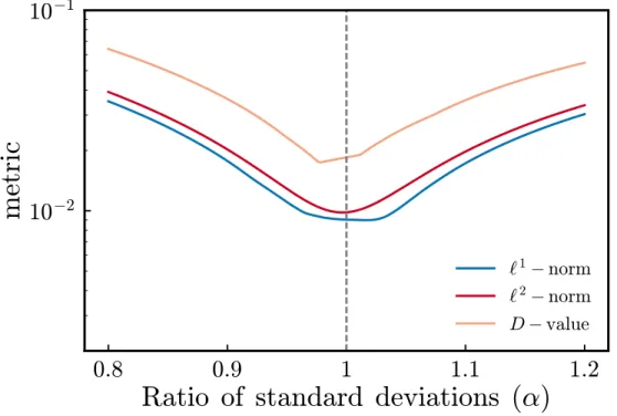
2.15 The 3 different metrics as a function of σphot. . . 57
2.16 RMS(β−b) as a function of Ns. . . 60
2.17 RMS(β−b) as a function of µspec. . . 61
3.1 Redshift-magnitude plot of the 3 samples for all fields. . . 81
3.2 Redshift-magnitude plot of the 3 samples for the remaining 2 fields. . . 82
3.3 Q-Q plot example. . . 85
3.4 Summed PDFs for a single magnitude bin from all 6 groups. . . 86
3.5 Summed PDFs for the 6 groups. . . 87
3.6 `2-norm vs dz for the six groups. . . 89
3.7 `2−norm vs γ for the 6 groups. . . 91
3.8 Q-Q plots for the 6 groups. . . 94
3.9 `2-norm vs fop for the six groups. . . 95
3.10 [DK: Scatter plot zweight vs zspec]. . . 97
3.11 σNMAD vs fco for 3 samples. . . 99
3.12 Fr´echet Distance.. . . 102
3.13 Optimized PDFs of 6 groups and 3 combination methods. . . 105
3.14 `2-norm vs. fop for the 3 samples and combination methods. . . 107
3.15 `2-norm vs fop for the 3 samples and 3 best combination methods. . . 108
3.16 σNMAD vs. fO for the 3 samples and combination methods. . . 109
3.17 σNMAD vs. fO for the 3 samples and 3 best combination methods. . . 110
3.18 Optimization Procedure Diagram. . . 112
4.1 The data and random samples for the 3 fields. . . 120
4.2 Redshift-magnitude plot of the 3 morphology types. . . 121
4.3 Projected correlation functions. . . 125
4.4 Projected correlation functions for irregulars. . . 126
4.5 Parametersr0 and γ for spheroids and disks. . . 129
1 INTRODUCTION
Our view of the universe has drastically changed over the past one hundred years or so. For millennia ancient civilizations had developed various mythological theories regarding the start and evolution of the cosmos as was known to them. For most of the recorded history humankind believed that our planet was the center of the universe, and all objects on the night sky revolved around it. Then, with the help of Galileo, Copernicus, and Kepler, astronomers shifted their theories towards a Heliocentric universe. Although this was a huge step in the right direction of the true picture, up until the beginning of the twentieth century, astronomers believed that all celestial objects that were visible at the time were part of our Galaxy, the Milky Way. Then, it became clear that the ”nebulae” which were known to them, were too far away to belong to the Milky Way (Hubble (1926), Hubble (1936)), and extragalactic astronomy was born. Soon after, with the help of technological advancements other galaxies were observed and cataloged, which led to a better understanding of the cosmos.
Today we know that our galaxy is only a drop in the vast ocean of galaxies in our universe, and the visible components of galaxies represent a small fraction of the 5% of the total mass-energy content of the Universe that consists of ordinary or ”baryonic” matter. Another 25% of the total mass-energy content is made up of a component known as dark matter; it interacts with baryonic matter primarily or exclusively via the gravitational force. Finally, the nature of the remaining 70% is also unknown to us today; it appears to be responsible for the observed accelerating expansion of the universe, and is generally labelled
Due to gravitational instabilities, baryonic matter collapses wherever the density is suffi-ciently high, forming dense structures such as galaxies, which in turn can group together to make up the largest gravitationally bound structures in the universe, called galaxy clusters. The mechanisms responsible for the formation of galaxies are yet to be fully understood; how they evolve with time is less well known. In order to make any progress towards such discoveries, we first need to identify and classify the objects of interest, which is why we present a brief introduction of the wide variety of galaxies in the following section.
1.1 CLASSIFYING GALAXIES
Galaxies have been observed to have a wide range of properties such as different ages, sizes, shapes, and colors even at constant mass; the reasons for this large variety are still not very clear. One thing that is apparent is that these properties are not entirely independent from one another. That is, the most massive galaxies tend to be older, redder, larger in size, and more commonly elliptical in shape. On the other hand, lower-mass galaxies tend to be younger, bluer, somewhat smaller in size, and disk shaped or irregular/peculiar. It is fairly certain that these properties of galaxies and how they evolve with time depend not only on baryonic matter and its distribution in the universe, but also on the properties of dark matter and dark energy, which is why the study of galaxies is of utmost importance for the study of the universe itself and therefore, cosmology. It is only natural for their study to start with some of their most obvious properties, such as their shape and color.
1.1.1 Galaxy Morphology
Since before realizing that the nebulae observed in the night sky were individual galaxies themselves, astronomers were fascinated with the shapes of these large structures of the universe. They appeared to have very noticeable differences, but at the same time many of them appeared to be very similar. Therefore it was clear that they can be divided into groups of similar appearances, an endeavor that occupied some of the brightest astronomers
of the twentieth century, such as Wolf, Hubble, de Vaucouleurs, Reynolds, etc. While dif-ferent scientists used difdif-ferent ways of categorizing galaxies based on morphology, the most commonly known is the Hubble Sequence (HS; Hubble (1926), Hubble (1936), Holmberg
(1958), de Vaucouleurs (1958), van den Bergh (1960)), which initially separated them into three major categories: ellipticals (E), spirals (S), and irregulars/peculiars (Irr) [Figure 1.1]. We continue with a brief description of the main morphological types of galaxies; for more details we refer the reader to Section 2.3 of Chapter 2 ofMo et al.(2010), and Chapter 3 of Schneider(2006).
Elliptical galaxies received their name due to their isophotal curves being ellipses. They are generally very smooth systems with lack of structures and brightness profiles that decline continuously with distance from the center, described by the de Vaucouleurs profile. They appear to have various ellipticities, which is the reason why their labelling E is followed by the integer n, taking values between 1 and 7. This integer represents the galaxy’s ellipticity and is given by n= (1−b/a)·10, whereb/a is the minor-to-major axis ratio of the galaxy.
Spiral galaxies show very clear features known as spiral arms, hence the name of their category. The spiral arms may spring from a central nucleus in which case they are referred to as normal spirals and labelled S, or the arms could start from a central region that resembles a bar, in which case galaxies are called barred spirals and they are labelled SB. Members of both of these two subgroups are further subdivided into smaller groups based on the state of their spiral arms, with the three main subgroups being a, b, and c. Sa and SBa galaxies have closely coiled spiral arms, Sb and SBb ones have more open arms, and Sc and SBc ones have quite open arms. Later updates to the initial Hubble Sequence by Hubble himself, de Vaucouleurs, and Sandage, added more subclasses such as Sd, SBd, etc., which was possible due to greater details in images obtained from better observations.
Another subgroup of the HS is the one containing the so called S0 galaxies, which have similarities both with ellipticals and spirals. They have a lenticular shape and have sometimes been speculated to be galaxies in a transitional phase from spiral to elliptical galaxies. In
Figure 1.1 Hubble Sequence (HS) today, with elliptical galaxies on the left, and spiral galaxies on the right; S0 galaxies in the middle. Spiral galaxies separate into the regular (upper row) and barred (lower row) groups. As we go from left (early-types) to right (late-types), galaxies appear to be bluer in color due to young massive blue stars formed in spiral galaxies. Credit: NASA, ESA, M. Kornmesser
having plenty of similarities among them.
Finally, there is the group of irregular galaxies (Irr). They are galaxies with irregular shapes (hence the name of their class), meaning that they do not show any elliptical or spiral symmetries of any sort, and therefore constitute a separate group from them. This class often contains galaxies which are characterized as peculiar, usually consisting of galaxies that are in a merging state with one or more other galaxies and hence appear abnormal in shape.
An additional set of terminology used to describe galaxy types is a temporal one. Going from left to right on the Hubble sequence they are labeled as early-type, intermediate-type, and late type. This language is misleading, since it is not connected with the ages of galaxies. Instead, this terminology was borrowed from the classification of stars; short-lived, massive, blue stars placed on the left of the Hertzsprung-Russell (HR) diagram are considered early-type ones, whereas longer-lived, lower mass, red stars that appear on the right of the HR diagram are referred to as late-type stars. The early, intermediate, and late terms were based on early theories of the stages of the lives of stars. It is ironic to note that early-type galaxies (E/S0) are usually made exclusively of old, red, late-type stars, whereas late-type galaxies (Sc, SBc, Irr) often contain many young, blue, early-type stars. This shows again the unfortunate nature of this temporal nomenclature for galaxies; we emphasize that this characterization does not indicate in any way an evolution or a time scale of any kind.
1.1.2 Galaxy Color
Another important visual property of galaxies is their color, which is closely related to their constituents, i.e., dust, gas, and stellar populations. When a galaxy is primarily made of old, red stars, it will also appear reddish in color when observed. In contrast, if another galaxy includes young, blue stars, it will then appear to be more blue when observed than the previous case.
that is usually referred to as the color-magnitude diagram for galaxies, and is analogous to the H-R diagram for stars (de Vaucouleurs (1961)). In this diagram galaxies separate into two very distinct groups, with one group favoring bluer colors (i.e. lower values of B-V), and the other consisting of galaxies with redder colors (i.e., higher values of B-V).
Given that the calculation of the absolute magnitude of a galaxy requires the knowledge of its distance, the color-color plot is in some cases easier to construct in order to see this bimodality of galaxies. For it we plot the colors of galaxies in two separate bands versus the colors in two other bands, e.g., U-B vs. B-V. Since colors are constructed from the differences between magnitudes, which in turn are related logarithmically to the ratio of fluxes, any dependence on the distance cancels out, and therefore it is not needed. This of course is only true for nearby galaxies, since for distant galaxies their colors are shifted to the redder wavelengths, as we will discuss in a later section, in which case we need to estimate the rest-frame colors of galaxies. In the color-color plot the two separate groups of galaxies are again distinguishable, with galaxies belonging to the “blue cloud” or the “red sequence”, depending on their respective colors (Strateva et al.(2001);Blanton et al.(2005);
Schawinski et al. (2014)).
With the recent increase of data, scientists have also shown interest in region of the color-magnitude diagram that is referred to as the green valley, which is the region of transition between the blue cloud and red sequence. Recent studies have suggested (Licquia et al.
(2015)) that our own galaxy may be a member of this population.
Additionally, it has been noticed that the colors of galaxies are closely linked to other properties of them, such as their morphologies (Strateva et al.(2001)). For instance, galaxies in the red sequence tend to be early-type ones (E/S0), whereas the blue cloud usually consists of late-type ones (S/SB & Irr).
Besides morphology and color, galaxies can be separated based upon a variety of other properties, such as their star-formation rates, masses, sizes, etc. As we have already men-tioned, it is clear that these properties are not completely independent from one another, and their correlation is of great interest to the scientific community, since it could shed light towards the mechanisms that drive galaxy formation and evolution. One important aspect regarding galaxy properties is how they are affected by the environment where different
galaxies are observed. It appears that different types of galaxies of different characteristics are found in different regions of the universe; some favor low-density regions (the ’field’) whereas others favor groups and clusters of galaxies. The trends observed in the local uni-verse may change significantly as we look at more distant objects, since larger distances correspond to earlier times when structure and galaxies were less developed. Therefore it is crucial not only to study the dependence of galaxy properties on environment but also how it evolves with time.
Before we start our discussion regarding the structure of the universe and its evolution, we must first define one of the most important quantities in Astronomy that allows us to describe large distances and past times. This quantity is generally known as the redshift; we briefly introduce this concept in the following section.
1.2 REDSHIFT
As the name suggests, the term ’redshift’ refers to a shift of the emitted light of distant objects to larger (corresponding to redder) wavelengths. This can happen due to the Doppler effect when objects are moving away from us with peculiar velocities, or due to the expansion of the universe resulting in the stretching of wavelengths of light. The former can be significant only for the very nearby objects whereas the latter dominates for larger distances. Mathematically, redshift is defined as z = (λo− λe)/λe, where λo is the observed wavelength and λe is the emitted wavelength. In the case of nearby objects, this can be approximated by z ≈ v/c, where v is the object’s velocity with respect to the observer, and c is the speed of light. In this work we focus on distant galaxies, for which a more useful definition is the one related to the scale factor a(t). The scale factor is a function of time and determines the emitted and observed wavelengths mentioned above according to λo/λe= a(to)/a(te), where a(to) is the scale factor at the time of observation and a(te) the one at the time of emission of the
One way to estimate the redshift of a galaxy is by analyzing its spectrum, and observ-ing the shifts in emission and/or absorption lines from their restframe wavelength, which in general yields very accurate results (Newman et al. (2013); Weiner et al. (2005)). Unfortu-nately, the acquisition of the spectra of galaxies is not an easy task, since it requires long exposure times, while the number of objects that are targeted during each observation is limited, making it practically impossible for surveys such as LSST (Ivezic et al.(2009)). In addition, the most distant galaxies are too faint to be observed spectroscopically, since their light cannot be analyzed in detail.
On the other hand, distant galaxies can be observed using broadband photometry, which is the measurement of the fluxes of all objects in the field of view of the instrument using dif-ferent filters (Nayyeri et al.(2017);Stefanon et al.(2017);Guo et al.(2013);Galametz et al.
(2013)). With this method, many objects can be observed at the same time, and measure-ments are feasible even for faint objects, thus making it the only solution for large surveys such as the aforementioned LSST. Additionally, the flux measurements can be accomplished with much shorter exposure times than what is required for detailed spectra. The caveat to this is the fact that the information is less detailed; as a result the photometric redshifts of galaxies are not as precise as their spectroscopic counterparts.
Having defined redshifts, which serve as the primary proxy for time in our work, we continue by describing the formation of galaxies, their temporal (or redshift) evolution, and how this relates to the environment a galaxy is found in in the following section.
1.3 OVERVIEW OF GALAXY FORMATION AND EVOLUTION
There has been a long history of research related to the formation and evolution of galaxies and the physical processes responsible for their vast variety we observe in the local and distant universe today. The picture is still being developed, although great progress has been made during the past few decades in this field (Dressler (1980); Postman & Geller (1984); Goto et al. (2003); Sheth et al. (2006); Skibba et al. (2013)). In this section we provide a brief summary regarding the main mechanisms we now believe are playing important roles in
shaping the structure of the universe into what is found everywhere in the cosmos.
1.3.1 Formation
We start this section with an overview of structure formation; for more details we refer the reader to Section 1.2 of Chapter 1 of Mo et al. (2010), the basics of which we summarize here.
According to the standard model of structure formation (Peebles (1980)), during the first stages of the universe the slightly overdense regions of dark matter collapse due to self-gravity forming small structures, usually referred to as dark matter halos (or simply halos). Because dark matter is believed to be collisionless and interacts only gravitationally, this process happens very early in cosmological time, and the regions with higher density will collapse and evolve faster than the less dense ones. According to the hierarchical scenario (Frenk & White (2012)), which is the most commonly accepted one, smaller sized halos form initially and they act as hosts for baryonic matter to also collapse gravitationally and form galaxies. This happens when the gas in the progenitor clouds cools and the pressure gradient cannot sustain hydrostatic equilibrium, therefore leading to the collapse (Dalgarno & McCray (1972)).
Which mechanisms are predominantly responsible for this cooling depends on the char-acteristics of the environment and more specifically on the virial temperature (Tvir) of the
dark matter halo, which in turn depends on its mass (Mh). For massive halos with high
temperatures Tvir ≥ 107K gas is fully ionized, making Bremsstrahlung emission of free
elec-trons the main mechanism of cooling. In the regime of 104K <Tvir < 107K cooling happens
mainly through atoms that end up on the ground states by radiation emission or via the capture of free electrons by ions to form atoms followed by radiation emission. For lower temperaturesTvir < 104K, atoms are no longer ionized and cooling becomes very inefficient,
Compton scattering from the interaction of the free electrons with the cosmic microwave background photons (Kraljic (2014)).
When gas cools sufficiently, it will tend to gravitationally collapse, potentially leading to the eventual formation of a galaxy (Greif et al. (2008) ). While the details are still not entirely clear, it is understood that variations in the properties of the host dark matter halos as well as the influence of other galaxies will guide the formation of new galaxies and determine their characteristics such as their shapes, colors, star formation activities, etc. Based on observations of the early universe it is believed that the majority of the first galaxies formed were small in size and irregular in shape, with a small portion of them being spheroids, which could explain the existence of dwarf spheroidal galaxies we observe today, which contain populations of old stars.
If the initial cloud of gas within a dark matter halo had a significant angular momentum, the cooling and collapse of the gas could lead to the formation of a disk (Firmani & Avila-Reese (1999); Firmani & Avila-Reese (2003)). Further collapse of gas clouds within a disk can ignite star formation; the stars themselves can influence the surrounding gas by ejecting into it material and heavier elements produced in their interiors, a process called feedback. This process has been proposed to overcome difficulties that arise regarding the formation of disk galaxies, such as the angular momentum catastrophe (Maller & Dekel (2002)) and the overcooling problem (Benson et al. (2003)). The former refers to the fact that mechanisms such as the dynamical friction between baryonic and dark matter can lead to a significant angular momentum loss therefore the disk would not be sustainable, whereas the latter is related to the first calculations that showed that in an environment where the cooling of gas is efficient, it would lead to its accumulation in the central region of the new formed galaxy, resulting in a bulge rather than a disk shape. Feedback processes (especially feedback from early supernovae, or SNe) can overcome both of these difficulties, since the energy ejected can heat the gas and slow down its collapse in order to preserve the disk, while it can also eject low angular momentum material outside of the region of the forming galaxy, thus maintaining the required angular momentum. While supernova feedback (Meier(1999,2001);Schawinski et al.(2007)) in combination with the photoionization due to the UV radiation from massive early stars and quasars (Quinn et al. (1996);Gnedin (2000)) can prove to overcome some of
the difficulties, it cannot completely solve the issues related with the formation of disks in galaxies.
The existence of the other morphological types observed in the universe is believed to be due to the evolution of early galaxies into other types following various physical mechanisms which will be described in the subsection below. After that we will compare their relative strengths and regions of dominance of these different mechanisms.
1.3.2 Evolution
As described above, the hierarchical bottom-up model suggests that smaller structures formed first. Dark matter halos host galaxies which during the early dense stages of the universe will attract each other into forming pairs, groups, or even galaxy clusters, which are the largest virialized structures of ordinary matter in the universe, with densities much higher than the average. In these environments, galaxies can undergo a variety of processes which can evolve them into becoming members of different morphological types, or they can suppress the formation of new stars, as well as strip galaxies off their gas contents. We pro-ceed with a brief overview of the main mechanisms driving this evolution. For a more detailed discussion we refer the reader to Boselli & Gavazzi (2006); we summarize the mechanisms described in that work below.
One of the most important processes believed to be responsible for galaxy evolution is mergers between galaxies, in which two (or occasionally even more) galaxies can combine together, forming a single larger object. If the two initial galaxies involved are of similar mass, the merger is called major, and studies have shown that such a process can lead to the formation of elliptical galaxies, regardless of the morphology of the progenitor galax-ies (White (1978), Hernquist et al. (1993)). If on the other hand, one of the two merging galaxies is significantly more massive than the other, then the process is usually referred to as a minor merger, and the final product can have properties similar to the larger-mass
part of a cluster, something that is supported by various observations indicating that clus-ters have substructures resembling groups of galaxies within them (Colless & Dunn (1996);
Rines et al. (2003)). The stage of galaxies interacting and merging with each other before becoming members of a cluster is sometimes referred to as the preprocessing stage (Okamoto & Nagashima (2003);Mulchaey et al. (2005)).
During the interaction of galaxies with each other, tidal effects can significantly disturb them, influencing their properties. If a galaxy is not very compact but has a relatively large radius compared to its distance to other members of the cluster, its interactions with the other members can cause part of the gas from the outer regions of a galaxy to be removed from it, which would then lead to a decrease in its star formation (Byrd & Valtonen(1990),Okamoto & Nagashima(2001),Diaferio et al.(2001)). This process in combination with minor mergers could be responsible for the formation of lenticular galaxies in clusters, though it still cannot account for the observed lenticular galaxies in the field (Springel et al. (2001)).
In a massive galaxy cluster, the gravitational potential of the cluster itself can also have tidal effects on its members, causing disturbances to their structures and internal processes (Merritt (1984), Miller (1986)). It has been suggested that these tidal interactions can also cause part of the interstellar gas to be ejected from the galactic plane of a galaxy, though the fraction of gas actually ejected is usually not very significant. On the contrary, in such situations a large portion of the gas is expected to gather in the central regions of a galaxy, potentially forming bars, as well as inducing star formation and generally increasing its nuclear activity (Byrd & Valtonen (1990), Henriksen & Byrd(1996)).
Given that galaxies in dense clusters can have very high orbital velocities, it is very rare for them to actually merge in the central regions of the cluster, unless the galaxies’ velocities are reduced due to dynamical friction, which will eventually lead to their infall towards the center of the cluster where the largest galaxy of the structure usually resides. The eventual fate of such galaxies is to be swallowed by the very massive and large central galaxies, a process that is called galactic cannibalism (Nipoti (2017)). If on the other hand galaxies continue to have very high speeds, then their interactions with the other members will be very short-lived. Nevertheless the very frequent interactions in combination with the interaction with the cluster gravitational potential can lead to a change of galaxy properties
via a process called galaxy harassment (Moore et al.(1996,1998)). Depending on the size and mass of the initial galaxies this process has been suggested to be responsible for the evolution of spiral galaxies into S0s, as well as the evolution of lower size galaxies into dE, dSph and dS0 galaxies (Moore et al. (1999)). It should be noted that while the aforementioned processes have been proposed to have an important role in the transformation of spiral galaxies into S0’s, it is now believed that other mechanisms that we discuss below play a bigger part in this evolution.
In addition to the primarily gravitational processes described above, galaxies can also undergo a variety of hydrodynamical processes in dense environments such as clusters which can affect their evolution. The high-velocity galaxy members of a cluster can lose their ISM due to the ram pressure from the IGM of the cluster, a process known as ram pressure stripping (Gunn & Gott (1972)). Various simulations show that while this process can effectively strip the outer layers of gas in the disk of a galaxy, it is very unlikely to completely remove it. Its efficiency depends on various parameters with one of the most important being the inclination of the disk with respect to the direction of motion; disks perpendicular to their direction of motion experience greater ram pressure than disks that are parallel to the plane of the trajectory of the galaxy (Balsara et al. (1994);Abadi et al.(1999); Quilis et al.
(2000); Vollmer et al. (2000)). This process could also induce starbursts in a galaxy from the compression of the disk gas (Bekki & Couch (2003); Bekki et al. (2003)), which can eventually lead to reduced levels of gas in the galaxy. Therefore this mechanism could have some responsibility for evolving spiral galaxies into S0s as well as dwarf irregulars into dwarf spheroidals by removing the fuel for star formation (Schulz & Struck(2001)). Furthermore, some studies have shown that ram pressure stripping can cause instabilities in the disk of a galaxy that lead to the formation of spiral arms which in turn can carry angular momentum in the outer regions of the disk and form gas rings (Vollmer et al. (2001); Bekki & Couch
(2003)).
at different rates depending on whether the flow is laminar or turbulent Nulsen (1982). While ram pressure depends strongly on the IGM density and the orientation of the disk with respect to their direction of motion, viscous stripping efficiency is mainly proportional to the IGM temperature and can be efficient even for galaxies with disks that are parallel to plane of their motion. Both ram pressure and viscous stripping require high velocities to significantly remove gas from galaxies, therefore they are believed to be dominant in the central regions of clusters, where orbital velocities of galaxies are sufficiently large. When the temperature of the IGM happens to be very high compared to the velocity dispersion of a galaxy, then its gas contents can heat up and evaporate through a process characterized as thermal evaporation (Gunn & Gott (1972); Cowie & McKee (1977); Cowie & Songaila
(1977)). The effects of this process are stronger for higher IGM temperatures, but they are significantly reduced in the presence of strong magnetic fields (Cowie & Songaila (1977);
Sarazin (2009)). Unlike ram pressure and viscous stripping, this process can be effective even at typical galactic velocities within a cluster, removing the cold gas which can be fuel for star formation (Boselli & Gavazzi (2006)). This effect can therefore be at least partly responsible for the existence of quenched galaxies in clusters that are observed both locally and at larger distances.
Often galaxies have outer loosely bound halos of gas that act as sources for gas to slowly fall into a galaxy and keep star formation going. However, if during the life of a galaxy within a cluster this supply is removed, this would lead to the eventual end of star formation within a galaxy, a process also known as galaxy starvation or strangulation (Larson et al. (1980);
Treu et al.(2003)). This process has been proposed to be responsible for the formation of S0 galaxies from spirals (Balogh et al. (2000); Bekki et al. (2002)), as well as dwarf ellipticals from low-mass spiral/irregular galaxies (Boselli et al. (2008)). The reason for the second case is that dwarf ellipticals have been observed to have low star formation activities while they have stellar distributions (i.e., density of stars as a function of radius) that are quite different from those of massive ellipticals but similar to those observed dwarf spirals and irregular galaxies; therefore it makes sense to consider the latter as the progenitor galaxies of the former (Mayer (2010)).
1.3.3 Comparison of Evolution Mechanisms
The processes described above are not easily disentangled when studying the evolution of galaxies in the large variety of environments where they are observed in the local and distant universe. In many cases all of them may apply in the formation and evolution of galaxies in clusters, and their importance depends on many factors such as the distance from the cluster center; the size and density of the cluster; the size and density of the member galaxies; the IGM and ISM densities; temperatures and chemical compositions; etc. In this section we attempt to briefly separate these processes and their importance in order to gain a clearer picture of how galaxies may have evolved with time.
Processes such as galaxy-galaxy interactions, galaxy-cluster potential interaction, and galaxy harassment which dominate in a dense cluster environment can all heat up the disks of galaxies and cause them to increase in thickness, but they are not very efficient in removing the gas from the disks, except for cases of small, loosely bound objects. They can also cause perturbations that lead to the transfer of gas towards the central regions of galaxies, thus increasing their nuclear activities (Boselli & Gavazzi (2006)). This would in turn enhance the bulge to disk ratio, which renders these processes capable of explaining some of the morphological differences between S0 galaxies and spirals, though not the quiescence of star formation in the S0s. While galaxy-galaxy and galaxy-cluster potential interactions are more dominant in the central regions of dense clusters (r < 0.2Mpc), galaxy harassment is believed to be more effective outside of cluster cores (r > 0.5Mpc).
On the other hand, processes that involve interactions of galaxies with the hot IGM cannot boost the thickness of disks or increase the bulge-to-disk ratio. They can however strip part or sometimes even all of the gas in disks, which in turn leads to a decrease in star formation. Processes such as thermal evaporation and laminar viscous stripping depend on the same parameters, though the former is about three times more efficient than the latter (Boselli & Gavazzi (2006)). Ram pressure stripping and turbulent viscous stripping also
& Gavazzi (2006)).
As we have mentioned above, ram pressure and viscous stripping are favored in cases of galaxies with larger sizes and higher velocities, which is the case for the central regions of dense clusters. Thermal evaporation, on the other hand, does not require high velocities and can be efficient for smaller-sized galaxies; its effectiveness depends primarily on the IGM temperature (but not density, radius, or velocity). Hence this process is strong wherever the IGM temperature be high. Evaporation can be effective at all radii in a cluster, though it usually dominates outside of the cluster cores, since in the central regions of dense clusters ram pressure and viscous stripping have enhanced effectiveness. Additionally, this process is not expected to be very effective in lower-mass environments such as groups or diffuse clusters where the lower temperatures decrease its efficiency.
In conclusion, hydrodynamical processes are more efficient in regions where the IGM is denser and hotter; i.e., the central regions of a cluster (r < 0.2Mpc). Similarly, the interaction of galaxies with each other and with the cluster potential is strongest in the dense central region of the cluster (r < 0.2Mpc). On the other hand, interactions that involve galaxy starvation, galaxy mergers, and galactic harassment are all dominant in the outer regions of clusters (r > 0.5Mpc) or in group-like environments where the interaction times are longer, as the typical velocities of galaxies are lower at higher radii or in lower-mass systems.
1.4 THE MORPHOLOGY-DENSITY RELATION
It has been known for some time that different types of galaxies are more dominant in different environments. Dressler (1980) used 51 rich galaxy clusters to show that elliptical and S0 galaxies are more prevalent in regions of higher density than spiral galaxies. Postman & Geller (1984) verified this result showing an increase in the fraction of E and S0 galaxies with increasing surface density (as projected in the sky). Bamford et al. (2009) used about 100k galaxies from Galaxy Zoo and found that both the fraction of ellipticals as well as the fraction of red galaxies would increase in higher surface densities. This picture continued to be true even at larger redshifts as was shown by galaxies from the SDSS (York et al.(2000)),
where the picture was very similar up to a redshift of ∼ 0.5. This observation is commonly known as the morphology-density relation. This suggests that other properties such as star formation and structure, along with their responsible mechanisms, are also correlated with environment.
An interesting recent finding is that while galaxy structure and galaxy morphology are closely related, their dependence on environment and stellar mass differs significantly. van der Wel (2008) used data from the SDSS of 4594 galaxies and showed that morphology, defined by S´ersic index + ”Bumpiness” as was defined in Blakeslee et al. (2006), depends on the local environment at fixed mass. On the other hand, structure as defined only by S´ersic index was found to depend on mass and not on environment. Suppression of star formation could be responsible for this behavior as it should primarily affect the morphology rather than the structure of a galaxy. Poggianti et al. (2008) found similar results using data from the ESO Distant Cluster Survey (EDisCS) at higher redshifts z= 0.4−1. They showed that the morphology-density relation is equivalent to the star formation-density relation, although for each separate morphological class, the star formation properties they took into account did not appear to show any dependence on environment whereas the morphological properties did vary with environment. This is probably due to the declining fraction of mainly late-type spirals (Sc) in denser environments, whereas early-late-type spirals (Sa, Sb) showed similar distributions to S0 galaxies. Calvi et al. (2012) investigate at low redshift (0.03≤ z ≤ 0.11) how the different morphologies are affected by mass and environment. Their findings showed that for mass-limited samples, the fraction of late-type galaxies decreased smoothly when going from single galaxies to dense clusters, while the opposite happened to early-type ones. The morphology of intermediate mass galaxies did not show any dependence on the stellar mass, but rather on the global environment, whereas the most massive galaxies exhibited both a stellar mass and an environmental dependence of their morphologies. Alpaslan et al.(2015) used a volume-limited sample of galaxies extending up toz =0.213, and their results showed that stellar mass played a more important role in galaxy properties than the environment.
higher-density regions. Coil et al.(2008) again used data from the DEEP2 survey, but took a different approach by using projected correlation functions, and finding similar results. The existence of a color-density relation is not very surprising since elliptical galaxies tend to be redder in color than disk galaxies. Additionally, bright ellipticals are more massive, do not show any significant star formation, and are generally older. This makes them the best tracers of massive dark matter halos, since they group together in the dense environments of clusters which reside in the most massive dark matter halos. On the other hand, spiral galaxies tend to be more prevalent in the field, i.e., they tend to not be part of clusters. The question then arises whether the morphology-density or the color-density relation is more fundamental and which originated earlier. In order to shed light on these important yet unanswered questions, we need to observe what happens to the aforementioned relations at earlier cosmological times, which we continue to discuss in the following.
1.4.1 Exploring Density Trends at Higher Redshifts
One question of interest in extragalactic astronomy is whether the relations of galaxy prop-erties with environment observed locally still continue to exist at higher redshifts. There is evidence that suggests that at higher redshifts a larger fraction of spiral galaxies appears in denser regions of clusters, which has led to the belief that perhaps elliptical galaxies form from evolving spiral and irregular galaxies (Moran et al. (2007), Poggianti et al. (2008)).
Galaxies change their properties with time, but their evolution time scales are too vastly large for humans to be able to observe this directly. However, due to the fact that light has a finite speed, it takes some time for it to travel from a distant object to us; as a result, the farther away an object is, the longer the light travel time, and therefore the light of objects we observe today has been emitted in the distant past. We can use this to our advantage in order to study galaxy evolution in a statistical sense, i.e., we can observe galaxy populations at different distances (and thus at different look back times) to indirectly observe their evolution. In order to achieve this, a very large number of galaxies needs to be observed, in order to minimize statistical biases and uncertainties. Large surveys such as 2dFGRS (Lahav et al. (2002)), CANDELS (Grogin et al. (2011) and Koekemoer et al. (2011)), and
SDSS (York et al.(2000)), have observed thousands, hundreds of thousands, or even millions of objects in the night sky, while new upcoming surveys, such as LSST (Ivezic et al.(2009)) plan to observe galaxies of the order of billions in number, extending farther and farther away, up to the first stages of the evolving universe.
Apart from a wide variety of studies of galaxy properties in the local universe, there have been numerous papers on the topic of galaxy evolution at higher redshifts, investigating how galaxies have evolved with time; a number of them have explored the evolution in the relationship between galaxy properties and environment. For instance, Tasca et al. (2009) investigated the dependence on environment of galaxy properties up to redshift of z ∼1with the zCOSMOS redshift survey. Using volume-limited samples with selected luminosities, they found that the galaxy morphology-density relation was already in place at z ∼ 1, albeit flatter than at lower redshifts. This finding was in agreement with previous works (Capak et al.(2007)), as well as with studies of the color-density relation at similar redshift (Cooper et al. (2007); Coil et al. (2008)). These studies were able to show that around
z ∼ 1 red galaxies clustered more strongly with the overall population of galaxies than bluer ones, as would be expected if they are associated with denser regions. Furthermore,
Kawinwanichakij et al. (2017) used the FourStar Galaxy Evolution (ZFOURGE) survey to investigate how environment and stellar mass affect the star formation activity of galaxies in the redshift range 0.5 < z < 2.0. They showed that both stellar mass and environment play an important role in the quenching of galaxies at such high redshifts.
There are two main conclusions that can be drawn from this large variety of studies. First they make it clear that galaxies evolve differently in different environments, and second they show that the relationship between galaxy properties and the environments where they are found evolves over time. The purpose of this dissertation is to investigate the dependence of average environment on morphology up to high redshifts (z ∼ 3) using data from the CANDELS Collaboration. More specifically, we want to investigate how the picture seen in the local universe changes with redshift so we can better understand the mechanisms that
dark matter halos come together to form larger ones, and the galaxies they host are also brought closer together in the process to form groups and clusters, it makes sense to consider that different physical processes will play important roles in galaxy evolution at different epochs and in different environments. For instance at high redshifts we expect the gas in galaxies and clusters of a given mass to be denser and hotter; therefore processes such as ram pressure stripping and thermal evaporation could more rapidly deplete galaxies of their gas reservoirs which will in turn quench their star formation. Since thermal evaporation can effectively remove the gas from small-size galaxies provided that the cluster IGM temperature is sufficient, it is expected to play an important role in the depletion of cold gas and the subsequent quenching of star formation at early times, when galaxies are considered to be less massive and much smaller in size compared to their local counterparts.
Although these processes can generally change the gas contents and star formations of galaxies, that can eventually lead to redder colors, they are generally not very efficient at completely changing their morphologies. However, it should be noted that it takes ∼ 1Gyr
for a galaxy’s color to transform after star formation ceases; as a result quenching galaxies may not have had sufficient time to turn red at higher redshifts, therefore galaxies at earlier times are expected to be generally bluer when observed in their restframe.
On the other hand, while processes such as tidal interactions and galaxy harassment can also lead to losses of gas, they can potentially increase the thickness of the disks of galaxies, therefore contributing in the transformation of spiral galaxies into lenticulars. Addition-ally, mergers of galaxies would tend to lead to higher fractions of ellipticals at later times through major mergers. Finally, galaxy starvation could be responsible for the transforma-tion of dwarf spirals and or irregulars, found in abundance in the early universe, into dwarf spheroidals.
As we will present in detail in the chapters to follow, our work in general is able to sep-arate galaxies into three main morphological types: spheroids, which generally correspond to elliptical galaxies; disks, which would include spirals and lenticulars together; and irregu-lars which would include galaxies of irregular shape and/or with tidal tails. Comparing the distribution of these three types of morphologies at different redshifts can help us to explore the main processes responsible for galaxy formation and evolution at redshifts up to z ∼ 3.
We continue with an overview of this work in the section below.
1.5 DISSERTATION OVERVIEW
This work is focused on improvements to photometric redshift probability distributions and on the clustering strength of different morphological types of galaxies as a function of red-shift. Photometric redshifts are extremely important for the future of astronomy and im-provements to them are of extreme value. In the following chapter we present a statistical method we can apply to photo-z PDFs to improve their overall performance, incorporating both single-valued ”point” estimates of redshift, as well as statistics describing distributions, leading to more representative estimates of errors. This method makes use of the Q-Q plot (Wilk & Gnanadesikan(1968)), and provides information regarding biases, unrepresentative uncertainties, asymmetry problems, and faulty characterization of tails of the photo-z PDFs. We then continue in the next chapter by applying this method to data from the CAN-DELS collaboration (Grogin et al. (2011); Koekemoer et al. (2011)). The collaboration has produced six separate estimates of photo-z PDFs; we apply a calibration method based on the work described in chapter 2 to each of the six sets of results independently. We then test their performance using independent spectroscopic redshifts, and we observe a clear im-provement in all cases. Furthermore, we present 3 different methods of combining individual PDF estimates for a given object, which in turn lead to even better results when tested with these independent redshifts.
In the next chapter we calculate correlation functions, making use of the CANDELS photometric redshift and morphology catalogs. The redshift catalogs are constructed by using spec-z’s whenever available, 3D-HST grism-z’s (Momcheva et al.(2016)) if there is no spec-z information, and the improved photo-z’s developed in Chapter 3 if neither spec-z’s nor grism-z’s are available. The morphology catalogs are provided to the collaboration by
functions of each morphology type sample with the full galaxy sample within different redshift bins, in order to investigate how the morphology-density relation evolves with redshift.
The final chapter includes a detailed discussion about our results and findings, and the implications for theories of galaxy formation and evolution. We also present ideas of future work related to this study that can help to unlock the mysteries of the Universe.
2 IMPROVING PHOTOMETRIC REDSHIFT PROBABILITY DISTRIBUTIONS WITH THE QUANTILE-QUANTILE PLOT
2.1 INTRODUCTION
The natures of dark matter and dark energy are still unknown to us today. New and up-coming surveys designed to study these phenomena will characterize very large numbers of objects; for instance, the Large Synoptic Survey Telescope (LSST;Ivezic et al.(2009)) plans to observe billions of galaxies over almost half the sky. We can use the redshift of an object as a proxy for its distance or lookback time; we determine redshifts by evaluating the light we receive from a galaxy.
One way to estimate the redshift of a galaxy is by analyzing a detailed spectrum, which in general yields very accurate results. Unfortunately, the acquisition of galaxy spectra of galaxies is not an easy task, since for faint objects such as those studied by LSST very long exposure times are required to obtain an adequate signal-to-noise ratio, while the number of objects that are targeted during a given observation is limited by technical challenges. As a result it will be practically impossible to obtain spectroscopic redshifts (also referred to as spec-z’s) for the great majority of objects studied by LSST and other deep imaging surveys. Alternatively, distant galaxies can be characterized using broad-band photometry, which provides measurements of the fluxes through a particular filter for all objects in the field of view of an instrument. With this method, many objects can be observed at the same time, and good signal-to-noise is achievable even for very faint objects, making it the only feasible
The downside to this is the much smaller amount of information provided by broad-band imaging. As a result, inferences about the redshifts of galaxies from their photometry – commonly known as photometric redshifts or photo-z’s – are considerably less precise than their spectroscopic counterparts.
It is common for photometric redshift algorithms to estimate probability density functions (PDFs) for the photo-z of an object, since PDFs provide considerably more information than a single “point” estimate of redshift or than a point estimate plus assumed-Gaussian errors. PDFs and point estimates are closely related; it is common to estimate point values directly from photo-z PDFs. For instance, one could use the redshift at which the PDF has its greatest value (zpeak) or the first moment of the PDF (i.e., the PDF-weighted mean
of redshift, zweight; in some cases this may be calculated only using the highest peak of
the probability distribution) as a single estimate of the photometric redshift. When either of these point values are compared to independent spectroscopic redshift samples, one generally finds substantial scatter, as well as a significant fraction of “outlier” redshifts which are far from the estimated photo-z. It is not uncommon for photo-z estimates to be biased on average when compared to spectroscopic z’s.
Just as point estimates can have imperfections, the PDFs provided by existing photo-metric redshift codes have proven in the past to be unreliable, not meeting the statistical definition of a probability density function (Fern´andez-Soto et al. (2002),Hildebrandt et al.
(2008),Dahlen et al.(2013), etc.). One way this may be seen is by investigating uncertainty estimates derived from PDF measurements. If credible intervals (the Bayesian equivalent of confidence intervals) are properly constructed, then 68% of spectroscopic redshifts should lie within the 68% credible intervals of the corresponding photo-z PDFs, 95% of spectroscopic redshifts should lie within the 95% credible intervals, etc. The reality can be far from this scenario; in recent tests, the number of spectroscopic redshifts within a given credible region may be much higher or much lower than what would be expected if PDFs have been properly constructed, depending on the particular photo-z code and the size of the credible interval considered (Dahlen et al. (2013)).
In this paper, we present simple methods which can help to correct for low-order deficien-cies in the probability density functions output by photometric redshift codes, resulting in
better estimates of both point values and credible intervals. This is done using the Quantile-Quantile plot (also known as the Q-Q plot; Wilk & Gnanadesikan(1968)) constructed with a subsample of objects with spectroscopic redshift measurements as well as the corresponding photo-z PDFs of the same objects.
We take advantage of the fact that, if the photo-z PDFs fulfill the standard statistical definition of a probability distribution, then the values of the cumulative distribution func-tions (CDFs) constructed from the PDFs and evaluated at the actual spec-z’s of the objects should follow a uniform distribution from zero to one. When this is not the case, it is an indicator that the photo-z PDFs are imperfect. In this paper, we consider the impacts on the Q-Q plot of a bias in the PDFs (shifting them from the true PDF); an underestimate or overestimate of errors leading to PDFs that are too narrow or too broad; an inaccurate level of asymmetry in the PDFs (i.e., inaccurate skewness); or finally, cases where the tails of the PDFs are too large or too small (i.e., inaccurate kurtosis).
In a recent paper published while this paper was being written, Freeman et al. (2017) used Q-Q plots to investigate the impact of differences between the distribution of properties of objects with spectroscopic redshifts used to train photo-z algorithms and the properties of the objects to which the algorithms are applied, as well as to evaluate their methods for mitigating this effect. In this paper, we consider the utility of the Q-Q plot as a general tool for assessing photo-z PDF accuracy, as well as methods for optimizing PDFs using statistics based on these plots.
In Section 2.2 we explain in detail the methods we use to assess the quality of photo-z
PDFs, and present Q-Q results for a variety of simple cases to illustrate the information available. In Section 2.3 we describe how information from Q-Q statistics can be used to calibrate photo-z PDFs to more closely fulfill the statistical definition, and illustrate our methods with mock data. Finally, in Section 5.2 we summarize and discuss the findings of this study.
2.2 METHODS
In order to quantify the quality of photo-z PDFs, we make use of a commonly-used variant of a probability plot, commonly known as the quantile-quantile plot or Q-Q plot (Wilk & Gnanadesikan (1968)). The Q-Q plot is frequently used as a visual technique to assess whether a set of data follows a given distribution, and is constructed by plotting quantiles – that is, the value within a distribution that some particular fraction of all values are below – calculated from data (shown as the y axis) against a set of quantiles expected from theory (used as the x axis). Percentiles or quartiles are examples of quantiles, but in the Q-Q plot the fractions at which quantiles are defined may be distributed continuously.
In an ideal case where the data are drawn from the theoretical distribution and the num-ber of datapoints is large, the data quantiles should equal exactly the theoretical quantiles. In this scenario, since both the x values and y values are exactly the same, the plot should correspond to the unit line (i.e., the line from (x = 0,y = 0) to (x = 1,y = 1)); this can be used as a reference line that the Q-Q curve for a particular set of distributions can be com-pared to. The deviation from the unit line provides useful information about how the data differs from the expected distribution, which can then be used to recalibrate and improve the quality of PDFs, as we show below.
More specifically, the data quantiles we use to construct the Q-Q plot are the values of the photo-z cumulative distribution functions (CDFs) evaluated at the actual spectroscopic redshifts of objects of known z, where the CDFs are derived from the corresponding pho-tometric redshift PDFs (photo-z PDFs), compared to the expected quantiles for a uniform distribution (as this is the distribution expected for data values randomly drawn from the PDF corresponding to a given PDF). The Q-Q plot constructed from the photo-z CDFs evaluated at the spectroscopic redshifts of sample objects provides a test of whether the photometric redshift probability distributions meet the statistical definition of a PDF.
If the photo-z PDFs have erroneous moments (such as their mean, standard deviation, skewness, kurtosis, etc.) this causes signatures in the Q-Q plot. Photometric redshift prob-ability distributions can be off in a variety of ways. For instance, an error in the mean corresponds to the PDFs having a bias such that they are effectively shifted to the left or
to the right compared to the true PDF of redshifts. An error in the standard deviation of the PDFs implies that they are too narrow or too broad; this will have effects primarily on the size of credible intervals predicted from a PDF. A difference in the skewness results in the PDFs having a different symmetry (or asymmetry) when compared to the true distri-butions. Finally, a difference in kurtosis results in the PDFs having too small or too long tails, and therefore predicting more or fewer outliers than they should. All these four cases show unique features in the Q-Q plot, and we investigate them below, following a detailed description of how we construct Q-Q plots.
2.2.1 Construction of Quantile-Quantile Plots
In order to construct a Q-Q plot, we start by generating mock data for a sample of size of Ns =1000 objects, and for each object we generate a spec-z value from its true photo-z PDF. For simplicity, in this paper we generally assume the true PDF is the same for all objects in a sample and is represented by a perfect Gaussian distribution of mean µphot and standard deviation σphot. We can make this assumption without loss of generality, as the
Q-Q statistics are based upon the distribution of CDF values constructed from a particular object’s PDF and evaluated at its spectroscopic redshift; the details of that PDF cease to matter as soon as the CDF is evaluated (we illustrate this with a detailed test below). An example of a simple toy model photo-z PDF and an associated spectroscopic redshift (zspec)
is shown in Figure 2.1.
Using an assumed photo-zPDF (which may or may not correspond to the true PDF from which redshifts were generated) we construct the cumulative distribution function (CDF(z)), from the equation:
CDF(z)=
Z z
0
PDF(z0)dz0 (2.1)
Additionally, we calculate the data quantile for a given object, Qdata, using the spec-z
1.5
2
2.5
redshift
z
1
3
5
P
D
F
(
z
)
Figure 2.1 True photometric redshift Probability Density Function, PDF(z) of a hypothetical object. The red curve corresponds to a normal distribution with µphot = 2 and σphot =0.1,
which we assume to be the photometric redshift PDF for a particular object. The vertical grey dashed line represents the spectroscopic redshift of the same object, which is here assumed to be zspec =2.1.
as is illustrated inFigure 2.2.
We continue by calculating the quantiles of the CDF values for all the objects in the mock data sample, sorting the values in increasing order. Theoretically we expect the values of the quantiles to follow a uniform distribution from 0 to 1, since we expect 1% of the objects to have values of the CDF less than or equal to 0.01, 2% of them to have CDF values less than or equal to 0.02, etc. We then construct the Q-Q plot by plotting the calculated quantiles from our mock data versus the theoretical quantiles (which just correspond to the fraction of CDF values that are lower than the given value). For instance, if the CDF values are below 0.2 10% of the time, the (Qtheory,Qdata) pair (0.1,0.2) would be a point along the Q-Q curve, as 0.2 would be the CDF value that corresponds to the 0.1 quantile (or tenth percentile) in the distribution of CDFs.
In the ideal case, the data quantiles should exactly equal the theoretical values, and therefore the plot should correspond to the unit line. In practice, that will never be the case even if PDFs are perfectly known, since the data are randomly sampled, causing deviations of quantiles from the theoretical expectation.
In order to quantify the deviation of the Q-Q plot from the ideal diagonal line, we use the normalized`2−norm, which is the square root of the sum of the squares of the differences of the plotted Q-Q curve from the diagonal line at each Qtheory value (i.e., the Euclidean distance), normalized by dividing by the square root of the number of objects:
normalized `2−norm= v u u u u t Ns P i=1 |yi,data−yi,theory|2 Ns , (2.3)
whereyi,datais theyvalue in a plot for the true curve andyi,theoryis the theoretical expectation (corresponding to the unit line, in our case). The differences between the curve and the
1.5
2
2.5
redshift
z
0
0.5
0.841
1
C
D
F
(
z
)
Figure 2.2 Cumulative Distribution Function, CDF(z), for the hypothetical object from
Figure 2.1. The red curve indicates the cumulative distribution function corresponding to the PDF in Figure 2.1. The spectroscopic redshift of zspec =2.1 is indicated by the vertical
grey dashed line, while the horizontal grey line shows the quantile value for the given object, CDF(zspec)= 0.841.
at each point, normalized by dividing by the square root of the number of objects: normalized `1−norm= Ns P i=1 |yi,data− yi,theory| Ns1/2 . (2.4)
Another metric that can be used is the largest difference between the calculated curve and the reference line, which is analogous to the D-value used in the Kolmogorov-Smirnov test (or K-S test for short). The difference here is that the K-S D statistic is generally computed between the empirical CDF and the theoretical CDF, whereas we are comparing quantile-quantile curves to the unit line.
The `1−normand`2−norm are in general more sensitive than the K-S-like D-value, since they take into account information from the entirety of the curve, not only the largest difference. Furthermore, the `2−norm is more sensitive than the `1−norm , since larger differences are squared and affect it more, for much the same reasons that the mean of a distribution of points is affected more by outliers than the median.
An additional useful quantity we measure is the fraction of the objects of the sample for which the quantiles are very small (quantile≤ 0.0001), or very large (quantile≥ 0.9999). These values correspond to spec-z’s that fall outside of the main regions of their respective photo-z PDFs, such that they might be considered outliers. We label this fraction of objects as fop (the fraction-outside-pdf), and we exclude them from the construction of the Q-Q
plot, tracking their numbers separately.
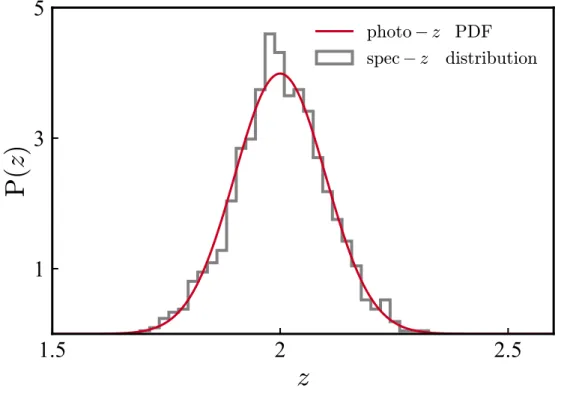
We start with the simplest case possible, where we consider all 1000 objects of our sample to have the same photo-z PDF, such that the spec-z’s are all generated from the same Gaussian distribution (Figure 2.3). We then calculate the quantiles for each redshift and after sorting them in increasing order, we plot them against a uniform distribution of values from 0 to 1 (Figure 2.4). The randomness in the generated spec-z’s results in the plotted curve deviating slightly from the ideal diagonal line, and the normalized `2−norm, though very small, is not identically zero. As expected, there are no outliers in this case, so
1.5
2
2.5
z
1
3
5
P
(
z
)
photo
−z
spec
−z
distribution
Figure 2.3 Example of the generation of a set of spectroscopic redshifts from photometric redshift PDFs. In this case, the spectroscopic redshifts (grey normalized histogram) are generated from the same distribution as the photo-z PDF (red solid curve), which is a Gaussian with µspec = µphot =2 and σspec = σphot = 0.1. For simplicity, the photo-z PDF is
chosen to be the same for all objects of the sample (in this case, Ns =1000). The histogram shows that although there is some randomness in the generation of the spec-z’s, such that the histogram has small deviations from the red line, the two distributions generally accord with each other.
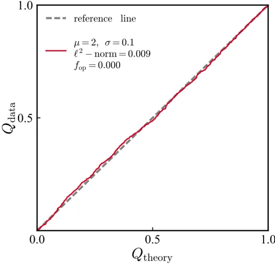
0.0
0.5
1.0
Q
theory
0.5
1.0
Q
da
ta
reference line
µ
= 2
, σ
= 0
.
1
`
2
−
norm = 0
.
009
f
op
= 0
.
000
Figure 2.4 The Q-Q plot for the same sample of Ns =1000 objects illustrated in Figure 2.3. The diagonal gray dashed line represents the ideal case, where the distribution of quantiles derived from the assumed photo-zPDF evaluated at the spec-z’s is perfectly uniform between zero and one. The red curve is constructed using CDF values from the same distribution actually used to generate the spec-z’s, as illustrated inFigure 2.3. As expected, the`2−norm is very close to zero and the outlier fraction fop is exactly zero for this case.