Variable Selection and Model Choice in Geoadditive Regression Models

Thomas Kneib, Torsten Hothorn & Gerhard Tutz

Variable Selection and Model Choice

in Geoadditive Regression Models

Technical Report Number 003, 2007 Department of Statistics

University of Munich

Variable Selection and Model Choice

in Geoadditive Regression Models

1 _{Institut f¨ur Statistik}

Ludwig-Maximilians-Universit¨at M¨unchen

Ludwigstraße 33, D-80539 M¨unchen, Germany

Summary.

Model choice and variable selection are issues of major concern in practi-cal regression analyses. We propose a boosting procedure that facilitates both tasks in a class of complex geoadditive regression models comprising spatial effects, nonparametric effects of continuous covariates, interaction surfaces, random effects, and varying coefficient terms. The major modelling compo-nent are penalized splines and their bivariate tensor product extensions. All smooth model terms are represented as the sum of a parametric component and a remaining smooth component with one degree of freedom to obtain a fair comparison between all model terms. A generic representation of the geoadditive model allows to devise a general boosting algorithm that imple-ments automatic model choice and variable selection. We demonstrate the versatility of our approach with two examples: a geoadditive Poisson regres-sion model for species counts in habitat suitability analyses and a geoadditive logit model for the analysis of forest health.

Key words: bivariate smoothing, boosting, functional gradient, penalised

splines, random effects, space-varying effects

1. Introduction

Generalized linear models (GLM) have become one of the standard tools for analyzing the impact of covariates on possibly non-Gaussian response vari-ables. A crucial question in setting up a GLM for a particular application is the choice of an appropriate subset of the set of available covariates, i.e., variable selection. In addition, one has to determine how to model the co-variate effects, a task we will refer to as model choice in the following. While variable selection and model choice issues are already complicated in linear models and GLMs and still receive considerable attention in the statistical

literature (see,e.g., George, 2000; Fan and Li, 2001; Zou and Hastie, 2005;

B¨uhlmann, 2006, for recent approaches and discussion), they become even

more challenging in geoadditive regression models including nonparametric effects of continuous covariates, spatial effects, or varying coefficient terms.

As an example, consider the case-study on forest health that will be

pre-sented in full detail in Section 5.2. Here we aim at analyzing the impact

of several covariates on the health status of trees measured as a binary in-dicator at a number of observation plots repeatedly over time. Instead of a linear predictor, previous analyses have suggested a model with a geoadditive predictor

η =x0β+f1(x1) +. . .+fq(xq) +f(x1, x2) +fspatial(s1, s2) +bplot,

wherex0βcontains usual linear effects of, for example, categorical covariates,

f1(x1), . . . , fq(xq) are smooth functions of continuous covariates such as time

or age of the trees,f(x1, x2) is an interaction surface,fspatial(s1, s2) is a spatial

is a plot-specific random effect.

Variable selection and model choice questions arising in such geoadditive models are as follows: Should a continuous covariate be included into the model at all and if so as a linear effect or as a nonparametric, flexible effect? Is the spatial effect required in the model, i.e., is spatial correlation present beyond the spatial variation accounted for by spatially varying covariates? Is the interaction effect required in the model? To answer these questions, we propose a systematic, fully automated approach to model choice and variable selection in geoadditive regression models utilizing a componentwise boosting procedure. Our approach generalizes previous suggestions for generalized

additive models byB¨uhlmann and Yu(2003) andTutz and Binder(2006) to

geoadditive models including space-varying and random effects.

After introducing extended geoadditive regression models and

compo-nentwise boosting in Section2, we propose suitable base-learners for a

vari-ety of modelling strategies in Section 3. The main ingredient are penalized

splines and their bivariate tensor product extensions. One major difficulty is to obtain base-learners that are comparable in complexity to avoid biased selection towards more flexible effects. The equivalent degrees of freedom of a nonparametric effect will be used as a general measure of complexity for the base-learners and a suitable re-parametrization will allow us to specify any desired degree of freedom for a base-learner.

To demonstrate the flexibility of the presented approach and the variety of model choice problems that can be accomplished with it, we present two case

studies in Section5. In the first example, an analysis of habitat suitability

correlation on variable selection as well as model choice in geoadditive models and models with space-varying coefficients. In the second example, forest health data are analyzed based on a complex model including nonparametric, spatial, interaction and random effects.

2. Generic Model Representation

Suppose that observations (yi,zi), i = 1, . . . , n, have been observed on a

response variable yi and a covariate vector zi comprising different types of

covariates. The conditional expectation of y is related to the covariates in

a GLM-type manner via_E(y|z) =h(η(z)), where h is the fixed inverse link

function. However, in contrast to GLMs the function η(z) is no longer

re-stricted to a linear function of the covariates but replaced by an additive

function ofr components η(z) =β0+ r X j=1 fj(z). (1)

The functions fj define generic representations of different types of

covari-ate effects, similar as in structured additive regression models considered in

Fahrmeir et al.(2004). To make the model formulation more concrete,

con-sider the following examples of functions fj: (i) Linear components f(z) =

flinear(x) =xβ,wherexis a univariate component of the vectorzandβis the

corresponding regression coefficient. (ii)Nonparametric, smooth components

f(z) = fsmooth(x), where x is a continuous component of z and fsmooth is a

function ofxsatisfying certain smoothness conditions. (iii)Spatial effects and

interaction surfaces f(z) = fspatial(x1, x2), where x1 and x2 are continuous

covariates andfspatialis a smooth, bivariate surface. In case of a spatial effect,

observation has been collected. (iv) Varying coefficient terms (Hastie and Tibshirani, 1993) f(z) = x1fsmooth(x2) or f(z) = x1fspatial(x2, x3), where

the interaction variable x1 is either a continuous or a binary covariate, the

effect modifiers x2 (and x3) are continuous covariates, and f(·) is either a

smooth univariate or a smooth bivariate function. If coordinate informa-tion is used as effect modifier, the resulting models are also called models with space-varying effects of geographically weighted regression models. (v)

Cluster-specific random effects f(z) =bc or f(z) =x1bc, where c is a cluster

index that relates an observation to the corresponding cluster the

observa-tion pertains to. For each group, a separate effectbc is specified which, under

appropriate distributional assumptions, defines either a random intercept or

a random slope of covariatex1.

The generic representation allows for a simplified formulation of complex models in terms of a unifying model description. Moreover, it tremendously facilitates the formulation of a generic componentwise boosting algorithm for variable selection and model choice, where each model component is repre-sented by a corresponding base-learner. In general, boosting can be inter-preted as a functional gradient descent method that seeks the solution of the optimization problem

η∗(z) = argmin

η(z)

E(ρ(y, η(z)), (2)

whereρ(·,·) is a suitable loss function such as the quadratic (L2-)lossρ(y, η) =

0.5|y−η|2 _{or the (log-)likelihood function. In practice, (2) is replaced by the}

empirical risk 1 n n X i=1 ρ(yi, η(zi))

and the boosting algorithm minimizes this quantity with respect to η. Af-ter initializing the function estimate with a suitable starting value ˆη[0]_{, the}

boosting procedure iteratively computes the negative gradient

ui =− ∂ ∂ηρ(yi, η) η=ˆη[m−1]₍z i) , i= 1, . . . , n

evaluated at the current function estimate and fits a base-learner g to u=

(u1, . . . , un)0. Since we are not only interested in obtaining an estimate of η

but mainly in model choice and variable selection, we utilize a componentwise

boosting algorithm. That means, we specify separate base-learners gj that

correspond to the functionsfj which defineη. Then, we select the best-fitting

componentwise base-learner j∗ = argmin 1≤j≤r n X i=1 (ui−gj(zi))2

and update the corresponding function estimate ˆfj to

ˆ f_j[m∗](·) = ˆf [m−1] j∗ (·) +νg [m] j∗ (·),

where ν ∈ (0,1] is a given step size, see B¨uhlmann and Hothorn (2008) for

a detailed derivation and examples. All other effects are kept constant, i.e., ˆ

f_j[m](·) = ˆf_j[m−1](·) for all j 6= j∗. All base-learners considered in Section 3

can be expressed as penalized least squares fitsgj(z) =X(X0X+λK)−1X0u,

whereX is a suitable design matrix (specifically introduced in Section3), K

is a penalty matrix andλ the corresponding smoothing parameter.

Variable selection and model choice then reduce to stopping the boosting

algorithm after an appropriate number of iterationsmstop. Within themstop

hence, the boosting algorithm provides a means of variable selection. Uti-lizing competing base-learners implementing different modelling possibilities for the same covariates also addresses the problem of model choice.

3. Base-learner for Geoadditive Regression Models

3.1 Nonparametric Effects

To derive appropriate base-learners for nonparametric effects of univariate continuous covariates, we first introduce a suitable nonparametric function estimate in the setting of scatterplot smoothing. Consider the simple model

ui =g(xi) +εi, εi ∼ N(0, σ2), i= 1, . . . , n, (3)

where g is a smooth function of x. A flexible yet parsimonious method to

estimate g is to approximate it by a linear combination of B-spline basis

functionsB_kl(x) of degree l, i.e.,

f(x) =

K

X

k=1

βkBjl(x),

whereβk are regression coefficients which scale the basis functions. In

prin-ciple, such an approach can be interpreted as a large linear model where the evaluations of the basis functions define the design matrix. This leads to the

matrix representation of (3) as u = Xβ+ε and the the regression

coeffi-cients could be estimated by least-squares. However, smoothness and form of the resulting function estimate crucially depend on the number of basis

functions employed. To overcome this problem, Eilers and Marx (1996)

in-troduced the idea of penalized splines, where a smoothness penalty is added to the least squares criterion when estimating the regression coefficients. A suitable penalty term can be constructed using an approximation to squared

derivatives of g(x) based on differences of the sequence of regression coeffi-cientsβ= (β1, . . . , βK)0. The d-th order derivative of a B-spline is essentially

determined by thed-th order differences leading to the penalty term

λP(β) =λ

K

X

k=d+1

∆d(βk)

where ∆d denotes thed-th order difference operator, e.g.,

∆1(βk) =βk −βk−1 or ∆2(βk) =βk−2βk−1+βk−2

for first and second order differences, respectively. Estimation of β is then

based on the penalized least squares (PLS) criterion

(u−Xβ)0(u−Xβ) +λP(β), (4)

The smoothing parameterλ ≥0 controls the flexibility of the function

esti-mate with large values enforcing smooth estiesti-mates and small values allowing for high flexibility. Employing a large number of basis functions yields a

flex-ible representation of the nonparametric effect g(x) where the actual degree

of smoothness can be adaptively chosen by varyingλ.

Seeking the minimizer of the PLS criterion (4) finally yields the

base-learner for nonparametric effects. To obtain a compact representation, we

rewrite the penalty term as the quadratic form λP(β) =λβ0Kβ where the

penalty matrix K is given by K= D0_dDd andDd is a d-th order difference

matrix of appropriate dimension. Then the penalized least squares estimate ofβ is given by ˆβ= (X0X+λK)−1X0u and the corresponding base-learner

can be represented in terms of the hat or smoother matrix (Hastie and

When performing model choice in semiparametric regression models, a crucial point in defining the nonparametric base-learner is the appropriate

choice of the smoothing parameter λ. If we choose λ too large, this will

lead to a bias in the boosting selection process preferring nonparametric effects over parametric effects due to their additional flexibility. In addition, we would like to select smoothing parameters that make the nonparametric effects of different covariates comparable in terms of their complexity. A natural measure built in analogy to model complexity in linear models is to

consider the trace of the smoother matrixSλas equivalent degrees of freedom

df(λ) = trace(Sλ) = trace(X(X0X+λK)−1X0) = trace((X0X+λK)−1X0X),

see Hastie and Tibshirani (1990). Degrees of freedom are a general

mea-sure for the complexity of a function estimates that allows to compare the smoothness even for different types of effects (e.g. nonparametric versus spa-tial effects) and for covariates measured on extremely different scales. If the

smoothing parameter is set to zero, df(λ) reduces to the usual complexity

measure of a linear model, i.e., the number of parameters describing the

spline (df(λ) = K). Positive values of λ lead to an effective reduction of

the number of parameters (df(λ)< K). However, even for very large values

of the smoothing parameter, we can not make df(λ) arbitrarily small since

a (d−1)-th order polynomial in x remains unpenalized by the d-th order

difference penalty (provided that the degree of the spline is larger than or

equal to the order of the difference penalty). Therefore, for differencesd≥2

we can not achieve df(λ) = 1 to make the nonparametric effect comparable

in the limiting case λ → ∞ since then the estimated effect is equal to a horizontal line and therefore effectively vanishes.

As a consequence, we have to modify the parametrization of the penalized

spline. The aim is to split the functiong(x) into a parametric part capturing

the (d−1)-th order polynomial that remains unpenalized and the deviation

from this polynomial gcentered(x), i.e.,

g(x) =β0+β1x+. . .+βd−1xd−1+gcentered(x). (5)

We can then assign the parametric effects describing the polynomial part to the usual linear effects and treat each of them separately using a para-metric base-learner. For the deviation part one can choose the smoothing parameter such that it has exactly one degree of freedom despite still being a nonparametric effect. Additionally, this re-parameterization has the advan-tage that the boosting algorithm provides a possibility to check whether the nonparametric modelling approach is needed, simultaneously with answering

the question of whetherxhas any influence on the response at all. If none of

the components in (5) is selected, then xhas obviously no effect. If only the

parametric components are selected, no nonparametric component is needed and the effect can fully be explained in a simplified model with parametric

effects only. We will illustrate this point in the applications in Section 5.

Note that decomposition (5) is similar in spirit to the truncated power

se-ries basis for polynomial splines but using a B-spline based decomposition retains the advantageous numerical behavior of this basis. Technically, the

decomposition of g(x) is achieved by decomposing the vector of regression

et al. (2004) for a detailed description in the context of mixed model based estimation of geoadditive regression models.

3.2 Spatial Effects and Interactions

For spatial effects based on continuous coordinate information (x1, x2) or

bivariate interaction surfaces of continuous covariates (x1, x2), we extend the

concept of penalized spline base-learners to two dimensions. Therefore, we first replace the univariate basis functions by their tensor products, i.e.,

gspatial(x1, x2) = K1 X k1=1 K2 X k2=1 βk1,k2Bk1,k2(x1, x2)

whereBk1,k2(x1, x2) =Bk1(x1)Bk2(x2),see alsoDierckx(1993) and in

particu-larWood(2006) where basis functions and products are discussed extensively.

In a similar way as for univariate nonparametric effects, this leads to a

repre-sentation of the vector of spatial effects as the product of a design matrixX

containing the evaluations of the tensor product basis functions and a vector of regression coefficientsβ= (β11, . . . , βK1,1, . . . , β1,K2, . . . , βK1,K2)

0_{,which is}

the vectorized representation of the bivariate field of regression coefficients. To construct a penalty term in analogy to univariate penalized splines as in

Eilers and Marx (2003), we consider separate penalties in x1 and x2

direc-tion first. The former can be obtained by constructing a univariate penalty

matrix K1 of dimension (K1 ×K1) and applying this matrix to each of the

subvectors of β corresponding to a row in x1 direction. In matrix notation,

this can be facilitated by blowing upK1based on the Kronecker product with

aK2-dimensional identity matrix, yielding the penalty termβ0(K1⊗IK2)β. Similarly, a penalty term inx2-direction is obtained asβ0(IK1⊗K2)β.Note

pre-multiplied with the identity matrix due to the ordering of the elements inβ. Summing up both components finally leads to the bivariate penalty term

λβ0Kβ=λβ0(K1⊗IK2 +IK1⊗K2)β

which penalizes variation in both x1 and x2 direction. A base-learner for

spatial and interaction effects is then given by Sλ = X(X0X+ λK)−1X0

which resembles the base-learner for univariate effects despite the increased number of regression coefficients involved in the description of surfaces.

As for univariate nonparametric smoothing, the spatial effect has to be decomposed into a parametric component representing the unpenalized part of the function estimate and the penalized deviation. From the construction of the penalty term it can be deduced that the unpenalized part is the tensor product of the univariate unpenalized parts. For example, in case of second

order differences in both x1 and x2 direction, a polynomial of degree one

remains unpenalized for both x1 and x2. The tensor product of these two

linear effects is then represented by an intercept, a linear effect inx1, a linear

effect in x2 and the interaction x1·x2. The deviation effect gcentered(x1, x2)

can then be constructed in analogy to the univariate setting, see Kneib and

Fahrmeir(2006) for details.

3.3 Varying Coefficient Terms

Varying coefficient terms (Hastie and Tibshirani, 1993) offer a special

way to include interactions between covariates of the form x1f(x2). This

can be interpreted as a flexible alternative to a parametric effect x1β, where

the constant effect β is replaced by a flexible effect function f(x2). As a

a continuous covariatex2 in subgroups defined by a binary variablex1 when

employing a predictor of the form

η(z) =. . .+fsmooth,1(x2) +x1fsmooth,2(x2) +. . .

If x1 = 0, the effect of x2 is given by fsmooth,1(x2) whereas for x1 = 1, the

effect is composed as the sumfsmooth,1(x2)+fsmooth,2(x2) andfsmooth,2(x2) can

be interpreted as the deviation effect ofx2 for the group defined by x1= 1.

Since fsmooth,2(x2) is again a flexible function, we represent the

corre-sponding base-learner in terms of a penalized spline yielding the expres-sion diag(x11, . . . , xn1)X∗β = Xβ for the vector of function evaluations

(x11g(x12), . . . , xn1g(xn2))0 in matrix notation. The design matrix X∗,

con-sisting of the B-spline basis functions representing the varying coefficient, is pre-multiplied by a diagonal matrix containing the values of the

interac-tion variable x1, yielding the row-wise scaled matrix X. The penalty term

needs not to be accommodated leading to the base-learner Sλ = X(X0X+

λK)−1_X0_{.In complete analogy we can set up models with space-varying}

ef-fectsx1fspatial(x2, x3) where fspatial is a bivariate penalized spline.

To allow for varying coefficient terms with one degree of freedom, restric-tions have to be imposed on the base-learner, leading, for example, to

x1g(x2) =β0x1+β1x1x2+. . .+βd−1x1xd2−1+x1gcentered(x2).

3.4 Random Effects

For clustered or longitudinal data, correlations between individual ob-servations can be accommodated by the inclusion of random effect terms, leading to a predictor of the form

where ci ∈ {1, . . . , C} denotes the cluster observation i pertains to. For

simplicity, we assume that the clusters are ordered consecutively from 1 toC.

In case of longitudinal data, the clusters are defined by individuals whereas

the repeated measurements forming the single observations are indexed byi.

We utilize the standard assumption of Gaussian random effects, i.e., bci,0 ∼

N(0, τ2

0) is a group-specific random intercept andbci,1∼ N(0, τ

2

1) is a

group-specific random slope.

The corresponding base-learner can then be cast into a similar framework as penalized splines and spatial effects. More specifically, the vector of

ran-dom intercept evaluations for the observationsi= 1, . . . , n can be expressed

as matrix-vector productX0b0 whereb0 = (b1,0, . . . , bC,0)0 is a vector

collect-ing all random intercepts and X0 is a zero-one incidence matrix that links

each observation with the corresponding random intercept. Random slopes can also be considered as varying coefficient terms with a random intercept as effect modifier. For the vector of effectsxi1bci,1 one obtains the expression

diag(x11, . . . , xn1)X0b1 = X1b1. A random effects base-learner is then given

bySλ= Xk(X0kXk +λkIC)X0k,k = 0,1, whereλk is a smoothing parameter

which is inverse proportional to the corresponding random effects variance.

4. Boosting in Geoadditive Regression Models

4.1 Generic representation

The generic representation of geoadditive regression models introduced in

Section2allows for a compact model formulation and description. However,

the concept is not limited to model description but can be continued for the

effects in a geoadditive regression model, the base-learners take the form

Sλ =X(X0X+λK)−1X0

whereλis an appropriately chosen smoothing parameter andKis a penalty

matrix. For fixed effects, the smoothing parameter is fixed at zero to obtain

an unpenalized fit. For all remaining effects,λis chosen such that the effect

has exactly one degree of freedom, i.e., df(λ) = trace(Sλ) = 1. Note, that the

degrees of freedom do not depend on the response variable. This is crucial for an efficient implementation of the boosting algorithm, since then the response variable is iteratively replaced by working residuals while proceeding through the fitting process. The desired value for the smoothing parameter can be obtained via a simple line search, although more sophisticated approaches can be used to speed up computations. The search for the smoothness parameter has to be performed only once in a setup step for the algorithm prior to the actual estimation loop.

4.2 A unified boosting algorithm

Utilizing the generic representation, the geoadditive regression model has the form η(z) =β0+ r X j=1 fj(z)

wherefj(z) represent the candidate functions of the predictor. A

componen-twise boosting procedure based on the loss function ρ(·) can be summarized

as follows:

1. Initialize the model components as ˆf_j[0](z) ≡ 0, j = 1, . . . , r. Set the

2. Increase m by 1. Compute the current negative gradient ui =− ∂ ∂ηρ(yi, η) η=ˆη[m−1]₍z i) , i= 1, . . . , n.

3. Choose the base-learner gj∗ that minimizes the L₂-loss, i.e. the

best-fitting function according to

j∗= argmin 1≤j≤r n X i=1 (ui−ˆgj(zi))2

4. Update the corresponding function estimate to ˆ

f_j[m∗](·) = ˆf

[m−1]

j∗ (·) +νSj∗u,

whereν ∈(0,1] is a step size. For all remaining functions set ˆf_j[m](·) = ˆ

f_j[m−1](·), j6= j∗.

5. Iterate steps 2 to 4 until m=mstop.

Typically, the loss functionρis given by the log-likelihood of the exponential

family under consideration. For the quadraticL2-loss, the negative gradient

equals the working residuals. Note that the boosting procedure used here

differs from LogitBoost as considered by Friedman et al. (2000) for binary

response and by Tutz and Binder (2006) for exponential family responses,

where in each boosting iteration a one step penalized likelihood fit with weights provides the base-learner. In the present approach, a penalized least squares fit to the current negative gradient vector is used instead.

To complete the specification of the boosting algorithm, appropriate

val-ues for the step-width ν and for mstop have to be defined. The step-width

fit. We use ν = 0.1 which has proven to be an appropriate default choice.

Selection ofmstopcan be based on AIC reduction: As long as a further

itera-tion decreases AIC, increase the iteraitera-tion index until a minimum is reached. To avoid local minima, it is typically favorable to fit a larger number of it-erations, trace the evolution of AIC with the iteration index and to use the

minimum as mstop only if it is far enough from the largest iteration that has

been fitted. Typically, AIC decreases much faster for the early iterations, whereas the increase after the minimum is much slower. This represents a convenient property of boosting procedures usually termed as slow

overfit-ting behavior. Even if we chose mstop considerably larger than the optimal

value, the resulting model would typically still fit the data reasonable well —

seeB¨uhlmann and Hothorn(2008) for an explanation andB¨uhlmann(2006)

for the derivation of AIC based on the output of a boosting algorithm.

The basic difficulty with an AIC-based selection of mstop is the

require-ment for evaluating the hat matrix defining the best-fitting base procedure

in every iteration. Since the hat matrix is of dimension n×n, these

com-putations will be slow if not infeasible for larger data sets. In such cases,

bootstrapping is an alternative strategy to determinemstop.

5. Applications

5.1 Habitat Suitability for Breeding Bird Communities

In our first application, we analyze counts of subjects from breeding bird communities collected at 258 observation plots in the “Northern Steiger-wald”, a forest area of about 10.000 hectare, located in northern Bavaria

habitat suitability and we will employ geoadditive extensions of log-linear Poisson GLMs to accomplish this task.

Originally, 43 species of diurnal breeding birds were sampled five times at each observation site from March to June 2002 using a quantitative grid mapping. To obtain conclusions regarding habitat quality that are more robust and universally valid, species having similar habitat requirements are

collected in seven structural guilds (SG) as defined in Table1. For each site,

31 habitat factors (see Table2) were measured, describing different aspects

of the habitat selection process.

Variable Selection in GLMs with Spatial Component In a first step, we investigated the impact of spatial correlation on variable selection prop-erties in generalized linear models. Therefore we fitted log-linear Poisson

regression models with the 31 influential variables from Table 2 entering in

linear form. Besides the purely linear model ignoring spatial correlation, we considered spatial models including a bivariate penalized spline surface of the coordinates. We utilized a first order difference penalty and 12 inner knots for each of the directions. In a first spatial GLM approach, five degrees of freedom were assigned to the spatial base-learner, which allows for consid-erably more flexibility of the spatial effect compared to the remaining linear effects in the regression model. To investigate the impact of this positive discrimination, we considered a spatial GLM where the spatial base-learner

is centered as described in Section 3 and can therefore be assigned exactly

one degree of freedom making it comparable to a parametric effect.

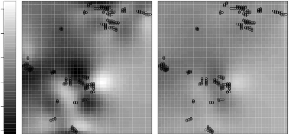
obtained from the three models. Comparing the non-spatial GLM and the high degree of freedom spatial GLM first, the inclusion of the spatial effect has a tremendous effect on variable selection, in particular reducing the in-clusion frequencies for several of the covariates, such as DWC. Reducing the degrees of freedom to one considerably changes the picture. Now most of the selection frequencies are relatively close to the corresponding value from the non-spatial GLM, although some reduced frequencies still reflect the in-fluence of spatial correlations on the selection process. Also, the selection frequency for the spatial effect itself is largely reduced when reducing the degrees of freedom. This, in turn, shows up in the resulting spatial effect

visualized in Figure1: Both for high and low degrees of freedom, the spatial

effect follows essentially the same pattern but is considerably lowered in the latter case. A qualitatively similar behavior is found for the other structural guilds as well, although in some cases, where the spatial effect is not very expressed, the inclusion frequency may even be increased in models with one degree of freedom.

Geoadditive Models In a next step, we extended the spatial GLM to a geoadditive model, where all covariates are allowed for possibly non-linear effects (except for LCA which has only 5 distinct values and is therefore not suitable for nonparametric modelling). All nonparametric effect base-learners are specified as penalized splines with second order difference penalty and 20 inner knots for the spline basis. The spatial base-learner is again included as a bivariate penalized spline with first order difference penalty and 12 inner knots for each coordinate. To differentiate between a flexible nonparametric

effect, parametric linear effect and no effect of a covariate, all nonparametric base-learners were centered around their unpenalized component, i.e. the linear part is effectively substracted from the nonparametric effect. Conse-quently, linear base-learners of all covariates are included separately into the boosting algorithm.

For structural guild 5, 24 out of the 31 possible covariates were identified

to have at least some impact on habitat suitability. Three out of them

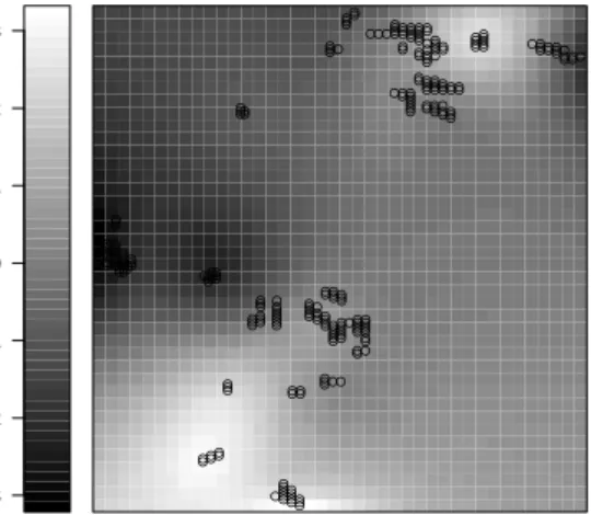
(DIO, GAP, AGR) only appeared as linear effects in the selected model, whereas the remaining 21 (GST, DBH, AOT, AFS, DWC, LOG, COO, CRS, HRS, OAK, COT, ALA, MAT, ROA, HOT, CTR, BOL, MSP, MDT, MAD, COL) appeared either as purely nonparametric or as the sum of a linear and a nonparametric component. Some selected effects (corresponding to the

variables selected most frequently) are visualized in Figure3and the spatial

effects estimated in the model is displayed in Figure2. Nonlinear modelling

of covariate effects also allows for deeper insight into the habitat selection process of the species. In stands with very low and very high DBH, gaps in the canopy result in higher abundance. A similar interpretation holds for COO where the effect is relatively flat over a wide range, corresponding to the fact that beeches do not need too much light for regeneration. For AOT, 100 years is the age of trees where most felling operations are observed. This results in gaps and following regeneration which leads to a higher abundance.

Space-Varying Effects Finally, we investigated whether some of the co-variate effects are spatially-varying and therefore considered varying coeffi-cient models where the continuous covariates enter as interaction variables

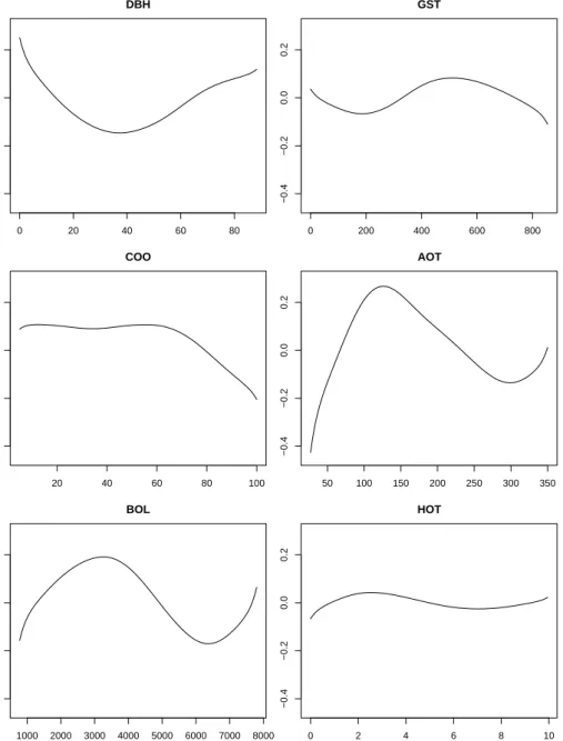
in a model with a bivariate surface of the coordinates as effect modifier. For all spatial base-learners, first order differences and 12 inner knots where ap-plied and a purely spatial effect without interaction variable was included in addition. All spatial base-learners are centered, allowing to assign one de-gree of freedom to each of them. The covariates where additionally included as linear effects, allowing to discriminate between the absence of any effect, a linear effect and a non-linear space-varying effect. For guild 3, 13 vari-ables (GST, AFS, LOG, COM, OAK, ALA, MAT, GAP, AGR, LCA, SCA, MAD, AGL) had exclusively linear influence on habitat suitability. For 12 further variables (DWC, CRS, PIO, GAP, AGR, ROA, SCA, HOT, BOL, MSP, MDT, SUL), spatially varying effects were identified, some of which

are shown in Figure 4. Interestingly, the spatial effect without interaction

variable was never selected, indicating that all spatial correlation is in fact covered by space-varying effects of some of the covariates. The effects for DWC and ROA correspond to a higher abundance of dead wood and road density, respectively, which also seems to modify the corresponding effect. Similarly, for BOL patchiness is higher in the north east due to small scale cutting resulting in increased heterogeneity and therefore longer borderlines.

5.2 Forest Health

The data set considered in the second application is more complex than the first example: The health status of beeches at 83 observation plots located in a northern Bavarian forest district has been assessed in visual forest health inventories carried out between 1983 and 2004. Originally, the health status is classified on an ordinal scale, where the nine possible categories denote

different degrees of defoliation. The domain is divided in 12.5% steps, ranging from healthy trees (0% defoliation) to trees with 100% defoliation. Since data become relatively sparse already for a medium amount of defoliation, we will model the dichotomized response variable defoliation with categories

1 (defoliation above 25%) and 0 (defoliation less or equal to 25%). Table 4

contains a brief description of the covariates in the data set.

Obviously, the collected data have both a temporal and a spatial com-ponent that has to be considered in the analysis. Moreover, due to the lon-gitudinal structure of the data, we are interested in estimating plot-specific

random effects. Previous studies described in Kneib and Fahrmeir (2006)

and Kneib and Fahrmeir (2008) also suggest the presence of interaction

ef-fects and non-linear influences of some continuous covariates. Based on these results we consider a logit model with candidate predictor

η(z) = x0β+f1(ph) +f2(canopy) +f3(soil) +f4(inclination)

+f5(elevation) +f6(time) +f7(age) +f8(time,age)

+f9(s1, s2) +bplot,

wherexcontains the parametric effects of the categorical covariates and the

base-learners for the smooth effects f1, . . . , f7 are specified as univariate

cu-bic penalized splines with 20 inner knots and second order difference penalty.

For both the interaction effect f8 and the spatial effect f9 we assumed

bi-variate cubic penalized splines with first order difference penalties and 12 inner knots for each of the directions. Finally, the plot-specific random

ef-fectbplot is assumed to be Gaussian with random effects variance fixed such

bivariate nonparametric effects are decomposed into parametric parts and nonparametric parts with one degree of freedom each. Since the number of

observations is too large for AIC-based choice of the stopping rule,mstop was

determined by a bootstrapping procedure.

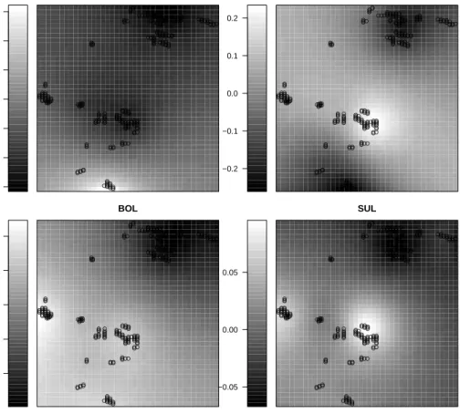
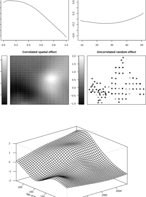
After applying the stopping rule, no effect was found for the ph-value, inclination of slope and elevation above sea level. The univariate effects for age and calendar time where strictly parametric linear but the interaction effect turned out to be very influential. The sum of both linear main effects

and nonparametric interaction is shown in Figure 5. The spatial effect was

selected only in a relatively small number of iterations whereas the random effect was the component selected most frequently. We can therefore con-clude that spatial variation in the data set seems to be present mostly very

locally, which is also confirmed by the results found in Kneib and Fahrmeir

(2008). For canopy density and soil depth nonlinear effects where identified

as visualized in Figure 5. In summary, our results resemble those found in

previous analyses but have the advantage that model choice and variable selection can be addressed simultaneously with model fitting.

6. Summary

Based on boosting techniques, an approach is presented allowing for variable selection and model choice in rather complex predictor settings in geoaddi-tive modelling. Since purely nonparametric estimation without structuring assumptions is hopeless, our approach starts with a set of candidate terms within the predictor which has a general additive form that includes para-metric as well as nonparapara-metric effect structures. The nonparapara-metric part

can be composed of arbitrary combinations of smooth, spatial, interaction, space-varying or random effects. To avoid selection bias towards nonpara-metric effects, a reparameterisation is introduced that allows to assign exactly one degree of freedom to all effects. The pre-selection of candidate sets can hardly be avoided but is not very restrictive in practical circumstances since it can be chosen very general when using boosting techniques. The proposed procedure automatically simplifies the pre-specified structuring.

All analyses are performed using an R(R Development Core Team,2007)

implementation of the presented methodology available to the interested

reader from package mboost (Hothorn et al., 2007). Its user-interface

(im-plemented in function gamboost()) facilitates the generic representation of

geoadditive models introduced in Section2. Thus, the transition from theory

to practice is leveraged by this common modelling language for geoadditive models.

References

B¨uhlmann, P. (2006). Boosting for high-dimensional linear models. The

Annals of Statistics 34, 559–583.

B¨uhlmann, P. and Hothorn, T. (2008). Boosting algorithms: Regularization,

prediction and model fitting. Statistical Science (accepted).

B¨uhlmann, P. and Yu, B. (2003). Boosting with L2 loss: Regression and

classification. Journal of the American Statistical Association 98, 324–

Dierckx, P. (1993). Curve and surface fitting with splines. New York: Oxford University Press.

Eilers, P. H. C. and Marx, B. D. (1996). Flexible smoothing using B-splines

and penalties. Statistical Science 11, 89–121.

Eilers, P. H. C. and Marx, B. D. (2003). Multivariate calibration with

temperature interaction using two-dimensional penalized signal regression.

Chemometrics and Intelligent Laboratory Systems 66, 159–174.

Fahrmeir, L., Kneib, T., and Lang, S. (2004). Penalized structured additive

regression: A Bayesian perspective. Statistica Sinica 14, 731–761.

Fan, J. and Li, R. (2001). Variable selection via nonconcave penalize

likeli-hood and its oracle properties. Journal of the American Statistical

Asso-ciation 96, 1348–1360.

Friedman, J. H., Hastie, T., and Tibshirani, R. (2000). Additive logistic

regression: A statistical view of boosting (with discussion). Annals of

Statistics 28, 337–407.

George, E. I. (2000). The variable selection problem.Journal of the American

Statistical Association 95, 1304–1308.

Hastie, T. and Tibshirani, R. (1990). Generalized Additive Models. Boca

Raton, Florida: Chapman and Hall.

Hastie, T. and Tibshirani, R. (1993). Varying-coefficient models. Journal of

Hothorn, T., B¨uhlmann, P., Kneib, T., and Schmid, M. (2007). mboost:

Model-Based Boosting. R package version 0.6-2.

URLhttp://R-forge.R-project.org

Kneib, T. and Fahrmeir, L. (2006). Structured additive regression for

categor-ical space-time data: A mixed model approach. Biometrics 62, 109–118.

Kneib, T. and Fahrmeir, L. (2008). A space-time study on forest health. In

R. Chandler and M. Scott, editors,Statistical Methods for Trend Detection

and Analysis in the Environmental Sciences. New York: John Wiley &

Sons.

M¨uller, J. (2005). Forest structures as key factor for beetle and bird

commu-nities in beech forests. PhD thesis. URLhttp://mediatum.ub.tum.de

R Development Core Team (2007). R: A Language and Environment for

Statistical Computing. R Foundation for Statistical Computing, Vienna,

Austria. ISBN 3-900051-07-0. URLhttp://www.R-project.org

Tutz, G. and Binder, H. (2006). Generalized additive modelling with implicit

variable selection by likelihood based boosting. Biometrics 62, 961–971.

Wood, S. N. (2006). Generalized Additive Models: An Introduction with R.

Chapman & Hall / CRC, Boca Raton.

Zou, H. and Hastie, T. (2005). Regularization and variable selection via the

−6 −4 −2 0 2 4 ● ●● ●● ●● ●● ●●● ● ● ●● ●●● ●● ● ● ● ● ● ●● ●●●●●● ●●●●●●●●●●●●●●●● ● ●● ●●● ●●●●●●●●● ● ●●●●● ●● ● ● ●● ●●●●●●●●●●●●●● ●● ●● ●● ●●● ●● ●● ● ●● ● ● ● ● ● ● ● ●●● ●● ●● ●● ●● ● ●● ●●● ●● ● ● ● ● ● ●●●● ●●● ●●● ●● ● ●●●● ●● ●● ● ●● ●●● ●● ●● ●●● ●●● ● ●● ● ●● ● ● ● ● ●● ●●● ●●●●● ●●●●● ●● ● ●● ● ● ●●●●● ● ●● ●●● ● ●● ● ● ● ● ● ● ●●● ● ● ● ●● ●●● ●●●●● ● ●●● ●●●●●● ● ●● ● ● SG4: 5 df ● ●● ●● ●● ●● ●●● ● ● ●● ●●● ●● ● ● ● ● ● ●● ●●●●●● ●●●●●●●●●●●●●●●● ● ●● ●●● ●●●●●●●●● ● ●●●●● ●● ● ● ●● ●●●●●●●●●●●●●● ●● ●● ●● ●●● ●● ●● ● ●● ● ● ● ● ● ● ● ●●● ●● ●● ●● ●● ● ●● ●●● ●● ● ● ● ● ● ●●●● ●●● ●●● ●● ● ●●●● ●● ●● ● ●● ●●● ●● ●● ●●● ●●● ● ●● ● ●● ● ● ● ● ●● ●●● ●●●●● ●●●●● ●● ● ●● ● ● ●●●●● ● ●● ●●● ● ●● ● ● ● ● ● ● ●●● ● ● ● ●● ●●● ●●●●● ● ●●● ●●●●●● ● ●● ● ● SG4: 1 df

Figure 1. Guild 4: Estimated spatial effect in GLMs with with either high

−0.3 −0.2 −0.1 0.0 0.1 0.2 0.3 ● ●● ●● ●● ●● ●●● ● ● ●● ●●● ●● ● ● ● ● ● ●● ● ●●● ●● ●●●●● ●●●●● ● ● ● ●●● ● ●● ●●● ●●●●●●●●● ● ●●●●● ●● ● ● ●● ●●●●●●●●●●●●●● ●● ●● ●● ●●● ●● ●● ● ●● ● ● ● ● ● ● ● ●●● ●● ●● ●● ●● ● ●● ●●● ●● ● ● ● ● ● ●●●● ●●● ●●● ●● ● ●●● ● ●● ●● ● ●● ●●● ●● ●● ●●● ●●● ● ●● ● ●● ● ● ● ● ●● ●●● ●●●●● ●●●●● ●● ● ●● ● ● ●●●●● ● ●● ●●● ● ●● ● ● ● ● ● ● ●●● ● ● ● ●● ●●● ●●●●● ● ●●● ●●●●●● ● ●● ● ● SG5: Geoadditive Model

0 200 400 600 800 −0.4 −0.2 0.0 0.2 GST 0 20 40 60 80 −0.4 −0.2 0.0 0.2 DBH 50 100 150 200 250 300 350 −0.4 −0.2 0.0 0.2 AOT 20 40 60 80 100 −0.4 −0.2 0.0 0.2 COO 0 2 4 6 8 10 −0.4 −0.2 0.0 0.2 HOT 1000 2000 3000 4000 5000 6000 7000 8000 −0.4 −0.2 0.0 0.2 BOL

−0.4 −0.2 0.0 0.2 0.4 0.6 0.8 ● ●● ●● ●● ●● ●●● ● ● ●● ●●● ●● ● ● ● ● ● ●● ● ●●●●● ●●●●● ●●●●● ● ● ● ●●● ● ●● ●●● ●●●●●●●●● ● ●●●●● ●● ● ● ●● ●●●●●●●●●●●●●● ●● ●● ●● ●●● ●● ●● ● ●● ● ● ● ● ● ● ● ●●● ●● ●● ●● ●● ● ●● ●●● ●● ● ● ● ● ● ●●●● ●●● ●●● ●● ● ●●●● ●● ●● ● ●● ●●● ●● ●● ●●● ●●● ● ●● ● ●● ● ● ● ● ●● ●●● ●●●●● ●●●●● ●● ● ●● ● ● ●●●●● ● ●● ●●● ● ●● ● ● ● ● ● ● ●●● ● ● ● ●● ●●● ●●●●● ● ●●● ●●●●●● ● ●● ● ● DWC −0.2 −0.1 0.0 0.1 0.2 ● ●● ●● ●● ●● ●●● ● ● ●● ●●● ●● ● ● ● ● ● ●● ● ●●●●● ●●●●● ●●●●● ● ● ● ●●● ● ●● ●●● ●●●●●●●●● ● ●●●●● ●● ● ● ●● ●●●●●●●●●●●●●● ●● ●● ●● ●●● ●● ●● ● ●● ● ● ● ● ● ● ● ●●● ●● ●● ●● ●● ● ●● ●●● ●● ● ● ● ● ● ●●●● ●●● ●●● ●● ● ●●●● ●● ●● ● ●● ●●● ●● ●● ●●● ●●● ● ●● ● ●● ● ● ● ● ●● ●●● ●●●●● ●●●●● ●● ● ●● ● ● ●●●●● ● ●● ●●● ● ●● ● ● ● ● ● ● ●●● ● ● ● ●● ●●● ●●●●● ● ●●● ●●●●●● ● ●● ●● ROA −0.10 −0.05 0.00 0.05 0.10 ● ●● ●● ●● ●● ●●● ● ● ●● ●●● ●● ● ● ● ● ● ●● ●●●●●● ●●●●●●●●●●●●●●●● ● ●● ●●● ●●●●●●●●● ● ●●●●● ●● ● ● ●● ●●●●●●●●●●●●●● ●● ●● ●● ●●● ●● ●● ● ●● ● ● ● ● ● ● ● ●●● ●● ●● ●● ●● ● ●● ●●● ●● ● ● ● ● ● ●●●● ●●● ●●● ●● ● ●●●● ●● ●● ● ●● ●●● ●● ●● ●●● ●●● ● ●● ● ●● ● ● ● ● ●● ●●● ●●●●● ●●●●● ●● ● ●● ● ● ●●●●● ● ●● ●●● ● ●● ● ● ● ● ● ● ●●● ● ● ● ●● ●●● ●●●●● ● ●●● ●●●●●● ● ●● ● ● BOL −0.05 0.00 0.05 ● ●● ●● ●● ●● ●●● ● ● ●● ●●● ●● ● ● ● ● ● ●● ●●●●●● ●●●●●●●●●●●●●●●● ● ●● ●●● ●●●●●●●●● ● ●●●●● ●● ● ● ●● ●●●●●●●●●●●●●● ●● ●● ●● ●●● ●● ●● ● ●● ● ● ● ● ● ● ● ●●● ●● ●● ●● ●● ● ●● ●●● ●● ● ● ● ● ● ●●●● ●●● ●●● ●● ● ●●●● ●● ●● ● ●● ●●● ●● ●● ●●● ●●● ● ●● ● ●● ● ● ● ● ●● ●●● ●●●●● ●●●●● ●● ● ●● ● ● ●●●●● ● ●● ●●● ● ●● ● ● ● ● ● ● ●●● ● ● ● ●● ●●● ●●●●● ● ●●● ●●●●●● ● ●● ●● SUL

0.0 0.2 0.4 0.6 0.8 1.0 −0.6 −0.2 0.2 0.6 canopy density 10 20 30 40 50 −0.6 −0.2 0.2 0.6

depth of soil layer

−0.01 0.00 0.01 0.02

Correlated spatial effect

−1.0 −0.5 0.0 0.5 1.0 1.5 2.0 ● ● ● ● ● ● ● ● ● ● ● ● ● ● ● ● ● ● ● ● ● ● ● ● ● ● ● ● ● ● ● ● ● ● ● ● ● ● ● ● ● ● ● ● ● ● ● ● ● ● ● ● ● ● ● ● ● ● ● ● ● ● ● ● ● ● ● ● ● ● ● ● ● ● ● ● ● ● ● ● ● ● ● ● ● ● ● ● ● ● ● ● ● ● ● ● ● ● ● ● ● ● ● ● ● ● ● ● ● ● ● ● ● ● ● ● ● ● ● ● ● ● ● ● ● ● ● ● ● ● ● ● ● ● ● ● ● ● ● ● ● ● ● ● ● ● ● ● ● ● ● ● ● ● ● ● ● ● ● ● ● ● ● ● ● ● ● ● ● ● ● ● ● ● ● ● ● ● ● ● ● ● ● ● ● ● ● ● ● ● ● ● ● ● ● ● ● ● ● ● ● ● ● ● ● ● ● ● ● ● ● ● ● ● ● ● ● ● ● ● ● ● ● ● ● ● ● ● ● ● ● ● ● ● ● ● ● ● ● ● ● ● ● ● ● ● ● ● ● ● ● ● ● ● ● ● ● ● ● ● ● ● ● ● ● ● ● ● ● ● ● ● ● ● ● ● ● ● ● ● ● ● ● ● ● ● ● ● ● ● ● ● ● ● ● ● ● ● ● ● ● ● ● ● ● ● ● ● ● ● ● ● ● ● ● ● ● ● ● ● ● ● ● ● ● ● ● ● ● ● ● ● ● ● ● ● ● ● ● ● ● ● ● ● ● ● ● ● ● ● ● ● ● ● ● ● ● ● ● ● ● ● ● ● ● ● ● ● ● ● ● ● ● ● ● ● ● ● ● ● ● ● ● ● ● ● ● ● ● ● ● ● ● ● ● ● ● ● ● ● ● ● ● ● ● ● ● ● ● ● ● ● ● ● ● ● ● ● ● ● ● ● ● ● ● ● ● ● ● ● ● ● ● ● ● ● ● ● ● ● ● ● ● ● ● ● ● ● ● ● ● ● ● ● ● ● ● ● ● ● ● ● ● ● ● ● ● ● ● ● ● ● ● ● ● ● ● ● ● ● ● ● ● ● ● ● ● ● ● ● ● ● ● ● ● ● ● ● ● ● ● ● ● ● ● ● ● ● ● ● ● ● ● ● ● ● ● ● ● ● ● ● ● ● ● ● ● ● ● ● ● ● ● ● ● ● ● ● ● ● ● ● ● ● ● ● ● ● ● ● ● ● ● ● ● ● ● ● ● ● ● ● ● ● ● ● ● ● ● ● ● ● ● ● ● ● ● ● ● ● ● ● ● ● ● ● ● ● ● ● ● ● ● ● ● ● ● ● ● ● ● ● ● ● ● ● ● ● ● ● ● ● ● ● ● ● ● ● ● ● ● ● ● ● ● ● ● ● ● ● ● ● ● ● ● ● ● ● ● ● ● ● ● ● ● ● ● ● ● ● ● ● ● ● ● ● ● ● ● ● ● ● ● ● ● ● ● ● ● ● ● ● ● ● ● ● ● ● ● ● ● ● ● ● ● ● ● ● ● ● ● ● ● ● ● ● ● ● ● ● ● ● ● ● ● ● ● ● ● ● ● ● ● ● ● ● ●_{●●●●●●●●●●●●●●●●●●●●●●} ● ● ● ● ● ● ● ● ● ● ● ● ● ● ● ● ● ● ● ● ● ● ● ● ● ● ● ● ● ● ● ● ● ● ● ● ● ● ● ● ● ● ● ● ● ● ● ● ● ● ● ● ● ● ● ● ● ● ● ● ● ● ● ● ● ● ● ● ● ● ● ● ● ● ● ● ● ● ● ● ● ● ● ● ● ● ● ● ● ● ● ● ● ● ● ● ● ● ● ● ● ● ● ● ● ● ● ● ● ● ● ● ● ● ● ● ● ● ● ● ● ● ● ● ● ● ● ● ● ● ● ● ● ● ● ● ● ● ● ● ● ● ● ● ● ● ● ● ● ● ● ● ● ● ● ● ● ● ● ● ● ● ● ● ● ● ● ● ● ● ● ● ● ● ● ● ● ● ● ● ● ● ● ● ● ● ● ● ● ● ● ● ● ● ● ● ● ● ● ● ● ● ● ● ● ● ● ● ● ● ● ● ● ● ● ● ● ● ● ● ● ● ● ● ● ● ● ● ● ● ● ● ● ● ● ● ● ● ● ● ● ● ● ● ● ● ● ● ● ● ● ● ● ● ● ● ● ● ● ● ● ● ● ● ● ● ● ● ● ● ● ● ● ● ● ● ● ● ● ● ● ● ● ● ● ● ● ● ● ● ● ● ● ● ● ● ● ● ● ● ● ● ● ● ● ● ● ● ● ● ● ● ● ● ● ● ● ● ● ● ● ● ● ● ● ● ● ● ● ● ● ● ● ● ● ● ● ● ● ● ● ● ● ● ● ● ● ● ● ● ● ● ● ● ● ● ● ● ● ● ● ● ● ● ● ● ● ● ● ● ● ● ● ● ● ● ● ● ● ● ● ● ● ● ● ● ● ● ● ● ● ● ● ● ● ● ● ● ● ● ● ● ● ● ● ● ● ● ● ● ● ● ● ● ● ● ● ● ● ● ● ● ● ● ● ● ● ● ● ● ● ● ● ● ● ● ● ● ● ● ● ● ● ● ● ● ● ● ● ● ● ● ● ● ● ● ● ● ● ● ● ● ● ● ● ● ● ● ● ● ● ● ● ● ● ● ● ● ● ● ● ● ● ● ● ● ● ● ● ● ● ● ● ● ● ● ● ● ● ● ● ● ● ● ● ● ● ● ● ● ● ● ● ● ● ● ● ● ● ● ● ● ● ● ● ● ● ● ● ● ● ● ● ● ● ● ● ● ● ● ● ● ● ● ● ● ● ● ● ● ● ● ● ● ● ● ● ● ● ● ● ● ● ● ● ● ● ● ● ● ● ● ● ● ● ● ● ● ● ● ● ● ● ● ● ● ● ● ● ● ● ● ● ● ● ● ● ● ● ● ● ● ● ● ● ● ● ● ● ● ● ● ● ● ● ● ● ● ● ● ● ● ● ● ● ● ● ● ● ● ● ● ● ● ● ● ● ● ● ● ● ● ● ● ● ● ● ● ● ● ● ● ● ● ● ● ● ● ● ● ● ● ● ● ● ● ● ● ● ● ● ● ● ● ● ● ● ● ● ● ● ● ● ● ● ● ● ● ● ● ● ● ● ● ● ● ● ● ● ● ● ● ● ● ● ● ● ● ● ● ● ● ● ● ● ● ● ● ● ● ● ● ● ● ● ● ● ● ● ● ● ● ● ● ● ● ● ● ● ● ● ● ● ● ● ● ● ● ● ● ● ● ● ● ● ● ● ● ● ● ● ● ● ● ● ● ● ● ● ● ● ● ● ● ● ● ● ● ● ● ● ● ● ● ● ● ● ● ● ● ● ● ● ● ● ● ● ● ● ● ● ● ● ● ● ● ● ● ● ● ● ● ● ● ● ● ● ● ● ● ● ● ● ● ● ● ● ● ● ● ● ● ● ● ● ● ● ● ● ● ● ● ● ● ● ● ● ● ● ● ● ● ● ● ● ● ● ● ● ● ● ● ● ● ● ● ● ● ● ● ● ● ● ● ● ● ● ● ● ● ● ● ● ● ● ● ● ● ● ● ● ● ● ● ● ● ● ● ● ● ● ● ● ● ● ● ● ● ● ● ● ● ● ● ● ● ● ● ● ● ● ● ● ● ● ● ● ● ● ● ● ● ● ● ● ● ● ● ● ● ● ● ● ● ● ● ● ● ● ● ● ● ● ● ● ● ● ● ● ● ● ● ● ● ● ● ● ● ● ● ● ● ● ● ● ● ● ● ● ● ● ● ● ● ● ● ● ● ● ● ● ● ● ● ● ● ● ● ● ● ● ● ● ● ● ● ● ● ● ● ● ● ● ● ● ● ● ● ● ● ● ● ● ● ● ● ● ● ● ● ● ● ● ● ● ● ● ● ● ● ● ● ● ● ● ● ● ● ● ● ● ● ● ●

Uncorrelated random effect

calendar year

1985 1990

1995 2000

age of the tree

50 100 150 200 −2 −1 0 1 2

T able 1 Definition of str uctur al guilds. Name Descriptio n Sp ecies SG1 R eq uireme n t of sma ll ca v es, snags and habit at trees Ficedula albicollis, F. h yp oleuca, F. pa rv a SG2 R eq uireme n t of o ld b eec h fo rests Dendr o cop os me dius, D. minor SG3 R eq uireme n t of ma ture de ciduo us tr ees Sit ta eur opaea , Dendro cop os ma jor, P ar us caeruleus, C ert hia fa miliar is SG4 R eq uireme n t of re g ene ratio n Ph y lloscopus tro chilus, Aeg ithalo s cauda tus SG5 R eq uireme n t of regenera tion com bine d with plan ted co nif ers Ph yllo sco pus co llybita , T urdus merula, Sylvia atr -icapilla SG6 R eq uireme n t of co nif ero us tr ees R egulus ignica pillus , P arus a ter, Prunella mo du-lar is SG7 R eq uireme n t of co nif ero us sta nds R egulus re g ulus, P a rus crista tus

T able 2 Envir onmental variables: A bbr eviation, description, range, sour ce and inventory ar ea. Descriptio n Ra nge Sour ce In v en tor y V aria ble s at stand scale GST Gro wing sto ck p er g rid 0 -8 54m 3 /ha F o res t in v en to ry 0.0 5 ha DBH Mean diameter o f the larg est three trees 0 -8 8cm F or est in v en tory 0.0 5 ha A O T Ag e o f oldest tree 2 7-350 y F or est in v en tory 0.5 ha circle AFS Ag e o f forest stand 2 7-300 y F or est in v en tory stand lev el D W C Amo un t of de a d w o o d of co nif er s 0 -1 27m 3 /ha Additiona l in v en to ry 0.1 ha cir cle LO G Amo un t of logs p er g rid 0 -2 93m 3 /ha Additiona l in v en to ry 0.1 ha cir cle SNA Amo un t of sna gs and att ac hed dea d w o o d a t living trees p er grid 0 -2 92m 3 /ha Additiona l in v en to ry 0.1 ha cir cle COO Ca nop y o v er o v erstorey 5 -1 00% Estima tion in field 1 ha grid COM Ca nop y o v er middles torey 0 -6 0% Estima tion in field 1 ha grid CRS P ercen ta ge of co v er of regenera tion and shrubs 0 -9 5% Estima tion in field 1 ha grid HRS Mean heigh t o f reg enera tion an d shrubs 0 -1 0m Estima tion in field 1 ha grid O AK P ercen ta ge of oak tr ees 0 -4 0% Estima tion in field 1 ha grid COT P ercen ta ge of co nife rous tree s 0 -8 0% Aeria l pho to 1 ha grid PIO P ercen ta ge of pioneer tree s (Sal ix, Betula, P opulus) 0 -7 5% Estima tion in field 1 ha grid ALA P ercen ta ge of alder and ash trees 0 -6 0% Estima tion in field 1 ha grid MA T P ercen ta ge of co v er of matur e tr ees 0 -1 00% Aeria l pho to 1 ha grid GAP P ercen ta ge of gaps p er g rid 0 -1 9% Aeria l pho to 1 ha grid A GR P ercen ta ge of agr ic ult ural land p er g rid 0 -2 1% Aeria l pho to 1 ha grid R O A P ercen ta ge of roa ds p er g rid 0 -1 3% Aeria l pho to 1 ha grid LCA Num b er of larg e ca vities p er grid 0 -1 5n/ha Addit ional in v en tor y 0.5 ha circle SCA Num b er of small ca vit ie s p er g rid 0 -3 3n/ha Addit ional in v en tor y 0.5 ha circle HOT Ho llo w trees p er grid 0 -1 0n/ha Addit ional in v en tor y 0.5 ha circle CTR Num b er of ca vi ty trees p er ha 0 -1 4n/ha Addit ional in v en tor y 0.5 ha circle V aria ble s at landscap e sc a le RL L L eng th of road s at the landscap e lev el 9 92-12 64 7m Aeria l pho to 78 .5 ha cir cle BOL L eng th of pa tc h b orderlines 7 80-78 00 Aeria l pho to 78 .5 ha cir cle MSP Mean size of habit at patc h 3 926 8-26 17 86 Aeria l pho to 78 .5 ha cir cl e MDT P ercen ta ge of mature dec iduo us tree s at the landscap e lev el 1 9-97% Aeria l pho to 78 .5 ha cir cle MAD P ercen ta ge of me dium ag ed deciduous trees a t the la nds ca p e lev el 0 -6 9% Aeria l pho to 78 .5 ha cir cl e COL P ercen ta ge of co nife rous tree s at the landscap e lev el 0 -7 7% Aeria l pho to 78 .5 ha cir cl e A GL P ercen ta ge of agr ic ult ural land at the landscap e le v el 0 -4 1% Aeria l pho to 78 .5 ha cir cl e SUL P ercen ta ge of success io n a t the la nds ca p e lev el 0 -2 4% Aeria l pho to 78 .5 ha cir cl e

T able 3 Guild 4: R elative sele ction fr equencies of covariates in a non-sp atial GLM, a sp atial GLM with high de gr ees of fr ee dom for the sp atial comp onent, and a sp atial GL M with one de gr ee of fr ee dom for the sp atial comp onent . GST DBH A O T AFS D W C L OG SNA C O O non-spatia l G LM 0 0 0 0 .06 0 .3 0 0.0 1 0 spatia l with 5 df 0 0.0 2 0 0.0 1 0.0 5 0 0 .01 0 spatia l with 1 df 0 0 0 0.0 6 0.1 5 0 0 0 COM CRS HR S O AK COT PIO ALA M A T non-spatia l G LM 0 .03 0 .04 0 .03 0 .05 0 .06 0 0.0 4 0.0 6 spatia l with 5 df 0 0.0 1 0 0 0 0 0 .01 0 .05 spatia l with 1 df 0.0 3 0.0 2 0 .02 0.0 4 0.0 5 0 0 .03 0 .04 GAP A GR R O A LCA SCA HO T C TR RLL non-spatia l G LM 0 .03 0 0 0 .1 0 .07 0 0 0 spatia l with 5 df 0.0 1 0 0 .01 0.0 1 0.0 1 0 0 0 spatia l with 1 df 0.0 3 0 0 0.0 7 0.0 6 0 0 0 BOL MSP MDT MAD COL A G L SUL spa tial non-spatia l G LM 0 0 .06 0 0 0 .05 0 0 0 spatia l with 5 df 0 0 0 0 0.0 3 0 0 0 .76 spatia l with 1 df 0 0.0 4 0 0 0.0 4 0 0 0 .3

Table 4

Forest health data: Description of covariates.

Covariate Description

age age of the tree in years (continuous, 7≤age≤234) time calendar time (continuous, 1983≤time≤2004)

elevation elevation above sea level in meters (continuous, 250≤elevation≤480)

inclination inclination of slope in percent (continuous, 0≤inclination≤46) soil depth of soil layer in centimeters (continuous, 9≤soil≤51) ph ph-value in 0-2cm depth (continuous, 3.28≤ph≤6.05)

canopy density of forest canopy in percent (continuous, 0≤canopy≤1) stand type of stand (categorical, 1=deciduous forest, -1=mixed

for-est).

fertilisation fertilisation (categorical, 1=yes, -1=no).

humus thickness of humus layer in 5 categories (ordinal, higher cate-gories represent higher proportions).

moisture level of soil moisture (categorical, 1=moderately dry, 2=mod-erately moist, 3=moist or temporary wet).

saturation base saturation (ordinal, higher categories indicate higher base saturation).