New Approaches to Simultaneous Multislice Magnetic Resonance Imaging : Sequence Optimization and Deep Learning based Image Reconstruction

(1)

New Approaches to Simultaneous

Multislice Magnetic Resonance Imaging:

Sequence Optimization and Deep

Learning based Image Reconstruction

Dissertation

submitted to the Faculty of Physics and Electrical Engineering

University of Bremen, Germany

for the degree of

Doctor of Natural Sciences (Dr. rer. nat.)

Klaus Eickel

Referees:

Prof. Dr. Matthias G¨

unther

Prof. Dr. Tony St¨

ocker

(2)

(3)

You can actually suffer a little bit more going slowly than when you’re going really fast. A faster marathon might even be easier than a slow one, in terms of what it takes out of you mentally.

(4)

(5)

Abstract and Outline

Magnetic resonance imaging (MRI) is a versatile imaging modality in clinical diag-nostics. Despite the impressive range of application, a main drawback of MRI is its inherently low acquisition speed. However, scan time is crucial for many applications and also for an efficient utilization of MRI in clinical routine. Two developments have influenced MRI recently: Simultaneous multislice imaging (SMS) and deep learning (DL).

Simultaneous multislice imaging is a paradigm shift in MRI which has re-emerged in the early 2010’. It yields improved image quality compared to in-plane parallel imaging, because it benefits from increased signal-to-noise ratio and robustness for higher accelerations. SMS sequences accelerate data acquisition by undersampling along the slice dimension and specific algorithms allow reconstruction of these under-sampled data.

In the first part, SMS was extended to measure multiple image contrasts in contrast-enhanced dynamic MRI. Therefore, a bespoke MRI sequence was developed to accelerate segmented echo-planar imaging of three echoes. Dynamic in-vivo data with sufficient spatial coverage were acquired in an animal model. Data acquisition were fast enough to sample the arterial input function which is essential for phar-macokinetic modeling. Imperfections in the excitation of multiple slice and their relevance for reconstruction algorithms were closely investigated and evaluated for processing of multi-contrast data.

This work connects SMS and deep learning. Today, the application of deep learning in medicine assists decision making in medical diagnosis, analysis of radiologic data or personalized medicine in genomics [Fou16]. In magnetic resonance imaging (MRI) however, deep learning has just entered the stage. With two abstracts matching the search term ’deep learning’ at the ISMRM 2016, the number of abstracts rose to 42 in 2017 and to 139 in 2018 [Mag17a; Mag17b; Mag18]. Most of the early contributions to DL in MRI concern image processing and data evaluation. Image reconstruction itself is mostly conducted in standard fashioned way. Common algorithmic approaches applying deep neural networks for (some) processing steps have shown impressive results and can often be generalized to similar problems [Yos+14].

In the second part, the separation of overlapping slice content after SMS was per-formed by an artificial neural network. This novel reconstruction technique, termed

SMSnet, does not require any reference data for calibration of the MR machine’s receiver characteristics. Omitting the need for reference data could extend the use of modern accelerated imaging sequences to a broad spectrum of applications [Bil+18]. Potential and limitations of this approach were investigated in various experiments

(10)

Abstract and Outline

accounting for image quality, robustness, sensitivity and how the network generalizes. The discussion at the end summarizes and relates the results of this work to state-of-the-art techniques and recent developments in MRI and gives an outlook to future work on SMS and DL-based reconstructions.

(11)

Part I

(12)

(13)

1 The Role of MRI in Medicine

This chapter briefly reviews the historical development of radiology followed by an introduction to theobjects investigated by MRI in this work. These can be structures like bones or organ-tissue or physiological processes, mainly blood-flow and perfusion.

1.1 Radiology: From X-Ray to Modern Imaging

In 1895, the physicist Wilhelm Conrad R¨ontgen entered a new age in medical diagnosis. He first published the discovery of X-rays and their ability to penetrate some materials while being absorbed by others. Six years later, R¨ontgen received the first Nobel Prize in physics for his remarkable work. He radiographed an assistant’s hand live on stage [col00], and from these early times onwards radiology has become an important field of medicine where screening, diagnostics and monitoring lead to a detailed insight into the human body and its intricate physiology [SM14]. The ongoing development from glass plates over films to digital visualization of radiographic images has transited plain radiography into modern digital radiology providing not only tomographic images in versatile forms of visualization, but also information beyond plain anatomy serving as direct biomarkers or facilitating more accurate diagnoses in the clinical decision process [SM14]. This ‘success’ in more information should also be considered critically in some cases, because more information can sometimes lead to diagnostic confusion as well [SM14].

Aside the remarkable benefits of today’s radiology, many imaging modalities come with additional risks associated with the ionizing radiation to which patients are exposed to. Radiation safety procedures began soon after clinical radiology had been established, but radiation-induced damage remains a critical point for X-ray, computer tomography (CT) or positron emission tomography (PET).

Ultrasound (US) and, from the early 1980s onwards, MRI extend the spectrum of available modalities and offer alternatives which are free of harmful ionizing radiation. Nevertheless, each modality has its individual (dis-)advantages and they all have found their place in modern radiological routine.

MRI, however, might have revolutionized the field of radiology more than any other technique after the discovery of X-rays. The ability to image without ionizing radiation, the option for selectable range of contrasts, its flexibility to be adjustable for a wide range of clinical questions may be unique properties and reasons for the increasing popularity and importance of MRI in anatomical and physiological imaging [Bae+05; Ope17].

(14)

1 MRI in Medicine

1.2 Anatomy and Physiology

The following sections introduce the anatomical and physiological basics inside the human body. If not referenced explicitly otherwise, the given facts are based on [Ope17], where an extensive description can be found as well.

Anatomy (Greek anatom¯e, ‘to cut apart’ or ‘dissection’) is the study of the human body’s structure. These structures range in size from macro- to microscopic where microbiology ties in with the later one and observations require optical instruments. On the macroscopic scale unaided eyesight as well as modern radiological machinery are used to observe structures for pathological changes. While dissection and ex-vivo examination represent anatomy in a rather traditional manner, today’s in-vivo and often completely non-invasive anatomical observation is assisted by a number of imaging techniques including MRI.

Physiology (Greek physis, ‘nature ’ or ‘origin ’) can be considered a complementary discipline which studies the function of body’s structures. This includes the chemistry and physics of the structures of the body and how their interaction supports the functions of life. On one hand physiology can be macroscopic, e.g. to study the musculoskeletal system with focus on the movement of the body. On the other hand it can take processes on a smaller base into account and investigate, for example, molecular exchange or fluid dynamics like the blood flow and its distribution. As for anatomy, physiological observations can be radiologically aided by machines where MRI, among others, plays an essential role thanks to its high general flexibility.

1.2.1 Blood

Most functions for (human) life are non consciously controlled processes, but driven by a complex interplay of electrochemical, chemical or physical factors. Almost all physiological processes relate directly or indirectly to the cardiovascular system made up of the heart, vessels and blood. An intact cardiovascular system guarantees the primary functions of a healthy biological system. Therefore, imaging of responses of the cardiovascular system to physiological processes serve as a measurable parameter and sometimes direct biomarker for changes in the body. Blood, acting as the mediator of this system, delivers oxygen, transports nutrients, removes cellular wastes and other byproducts to removal organs, assists the immune response and preserves homeostasis. Blood can also transmit information through hormones released by endocrine glads into the bloodstream.

Blood itself is a connective tissue and unlike other connective tissues unique in a way because it is fluid. By being a connective tissue it is made up of cellular elements, including red and white blood cells, and an fluid extracellular matrix, the plasma. The plasma itself consists to about 8 % of suspended substances, mostly proteins, and to 92 % of water making it an excellent candidate to be imaged with MRI. Under

(15)

1.2 Anatomy and Physiology normal, healthy conditions blood has a stable temperature of about 38◦C, slightly above body temperature and a viscosity of 1.4 mN·s/m2.

1.2.2 The Vascular System and Perfusion

The heart pumps blood in a closed network of differently sized blood vessels. This subpart of the cardiovascular system which carries the blood throughout the body is called vascular system. Starting at the heart, blood streams away in the aorta, where arteries connect to and distribute blood to tissue, organs and even bones. The arteries branch into even smaller vessels, the arterioles, which finally branch into thin capillaries with a diameter of 5µm – 10µm. The exchange of oxygen, nutrients and wastes between blood and tissue takes place in these finest structures of the vascular system, the so-called capillary bed. The transportation of blood through the capillary bed is known as perfusion measured in _s_·ml_mg. The capillaries combine later on the venules which themselves merge into veins and through which the blood returns to the heart (Fig. 1.1).

The different vessels share many features, but also differ in some structural properties. The heart ejects blood into the major aorta and then surging in the vascular system. The differences in pressure let the blood flow and as such, this requires stronger vessel walls for the higher pressure at the beginning of the closed vascular system than at its end. Blood streams through the lumen, a hollow passageway inside the vessels, that is smaller in diameter in the arterial than the venous partition of the system to ensure correct pressure. The complex interaction of pressure, blood velocity, blood volume, vascular resistance and others is called hemodynamics. A simplified approach is to formulate the vascular blood flow by the law of Hagen-Poiseuille as laminar fluid dynamics. The role of the vessels diameter, the total cross-sectional area, blood pressure and velocity can be described well on a macrovascular scale. However, since blood cells with a approximate sizes of 6µm – 15µm and the capillaries are of similar size, fluid dynamics disappear. The mass movement of fluids into and out of the capillary bed requires additional transport mechanisms. As depicted in Figure 1.1, hydrostatic and osmotic pressure move fluid or suspension from the capillaries into the interstitial fluid, also known as tissue fluid, and vice versa. The osmotic concentration gradients are not determined by the erythrocytes, leukocytes and thrombocytes in the blood, rather, it is the plasma proteins that play the key role.

1.2.3 Angiogenesis

Angiogenesis is the creation of new vascular structure, i.e. blood vessels from existing ones. It is responsible for most blood vessel growth during development and vascularization of new formed tissue, but also in disease. The term cancer is broadly used to describe diseases caused by mutated, abnormal cells accompanied by uncontrolled cell division, fast proliferation and vessel growth. While mutations not

(16)

1 MRI in Medicine

Figure 1.1: a) The cardiovascular and pulmonary circulation where the heart center moves blood through the lungs and the vascular system. b) A zoomed, schematic illustration of the capillary bed with its connections to the arterial and venous vessel system. c) Interplay of hydrostatic and osmotic pressure driving the exchange processes in the capillary bed. Adapted from [Ope17] licensed by CC BY 4.0.

necessarily chase noticeable change in the cell function, mutations affection the key proteins directly impact the cell’s properties. These abnormal cells often lose the ability to proliferate orderly, which results in the formation of irregular tissue and vascular structures. Accumulations of abnormal cells and the resulting formation of tumors are often benign, but can become malignant, or cancerous. Cancerous tumors breach neighboring tissue, promote irregular angiogenesis, in particular on the capillary level and metastasize to other organs later on. Despite their chaotic order, tumors are not merely disorganized accumulations of cells, but have their own structures. Nevertheless, the fast growth of a tumor makes it vasculature porous with wide interendothelial junctions, heterogeneous and coarse in the capillary bed [Bae+05]. The vessels may also show discontinuous or even absent base membrane. All these factors favor leakage of solvents from the vasculature into the extravascular extracellular space (EES) [Jai87].

1.3 MRI in Radiation Oncology

Radiotherapy, a therapy where ionizing radiation is used to locally control or eliminate cancerous cells, is one of the most important therapies in nowadays cancer treatment [Bau+16]. Selection and contouring of the targeted tumor volume is an important challenge for successful radiotherapy [Bau+16]. Because of its excellent soft-tissue contrast, its harmlessness in terms of ionizing radiation and its versatility, MRI plays a key role for delineating the tumor volume, but also structures and organs at risk in

(17)

1.4 Accessing Physiological Parameters radiation therapy planning [Bae+05; Met+13]. While anatomical imaging has become an essential component in radiation oncology, the potential of physiological imaging to access radiobiological factors or biomarkers has only been partly revealed [Bau+16]. The so-called ‘Rs’ of radiotherapy determining the biological effectiveness of radiation are: radio-sensitivity or radio-resistance, hypoxia and reoxygenation, repopulation and redistribution. The reliable assessment of these ‘Rs’ is highly relevant for planning advanced radio-therapeutic treatments such as intensity-modulated ratio therapy (IMRT) and dose adaption between fractions to achieve tumor control and long-term survival [Bau+16].

By use of specific MRI techniques, physiological information such as tumor perfusion, vascular permeability, extracellular space tortuosity, metabolic status and hypoxia, which are potentially related to the ‘Rs’ can be obtained and support therapy planning [Des+09]. One essential component to assess physiological information by MRI is dynamic imaging, which requires fast acquisition methods to reflect physiological processes with timescales of a few seconds (Cha. 1.4). In particular, for MRI techniques where an exogenous substance, the so-called contrast agent, is injected, rapid sampling of the fluid dynamics in major vessels is crucial. Additionally, accelerated magnetic resonance (MR) acquisition strategies are desirable for most sorts of imaging protocols, either anatomical or physiological because the availability of MR machines is limited and clinical workflow is strict.

1.4 Accessing Physiological Parameters

As introduced in Section 1.2, blood flow and perfusion represent essential parameters of nearly all physiological processes and ,therefore, often serve as a biomarker for various clinical diagnoses [Sam16]. MRI techniques to access physiological parame-ters may be divided into exogenous and endogenous methods. In the first ones, an exogenous substance, a so-called contrast agent (CA), is injected into the vascular system and its distribution is traced. dynamic contrast-enhanced (DCE) and dy-namic susceptibility contrast (DSC) are well known methods to measure perfusion by contrast-enhanced MRI as described in more detail in Section 1.4.1. Contrary, methods which trace endogenous substances work non-invasively. Blood-oxygenation-level dependent (BOLD) imaging, which will be introduced in Section 1.4.2, is a well-known technique to access brain activity in functional magnetic resonance imag-ing (fMRI). For perfusion imagimag-ing, arterial spin labelimag-ing (ASL) is a MRI technique which used magnetically labeled blood to trace supply of tissue with blood [Det+92]. Although, many properties of ASL, e.g. non-invasive and repeatable, make it an appealing method, clinical ASL has still a limited spectrum of applications, such as brain or kidney perfusion [Als+15].

(18)

1 MRI in Medicine

1.4.1 Contrast-Enhanced Perfusion MRI in Oncology

The following section will give an brief introduction to dynamic contrast-enhanced MRI in research and clinical oncology. If not explicitly cited differently, this section refers to [Bae+05]. Further reading suggestions for image analysis from the beginning of CA-enhanced MRI [Ros+90], to the comprehensive issue of the so-called arterial input function (AIF) sampling [Cal13] as well as basic and advanced pharmacokinetic modeling [SB13] and perfusion MRI [Jah+14] can be found in the references. Yet, this work focuses on the acquisition of the MR signal rather than on its detailed analysis.

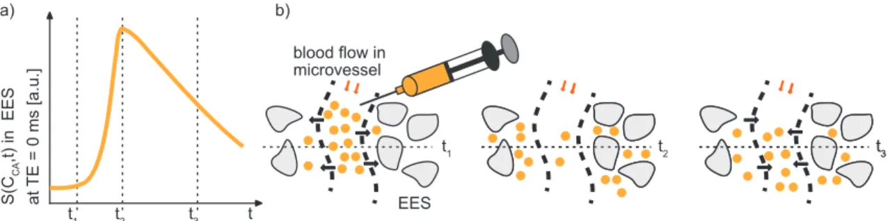
The first injection of a Gadolinium-based CA for MRI in a human volunteer was conducted in Berlin in 1983 to show resulting signal enhancement in the bladder [Loh+16]. The motivation for contrast-enhanced MRI and, in particular, its value for oncology arises from the variations in temporospatial enhancement patterns after CA-administration. Figure 1.2 depicts the temporal changes in the MR signal (a) and the diffusion by which CA-molecules may pass vessel walls and enter the EES to equalize intra- and extravascular CA-concentration (b). Over time, excretion by the kidneys reduces intravascular CA-concentration and the concentration gradient changes direction which results in back-diffusion of the tracer particles. This phase is called wash-out, because CA-molecules are gradually removed from the body. The dynamics in the MR signal reflect (abnormal) changes in microvascular structure and pathophysiology. These can be affected by various physiological factors including regional blood flow, perfusion, vessel density, permeability and surface area of endothelial membranes or size of the EES and its CA-concentration difference to the plasma. All these factors change, to a certain extent, from healthy tissue to tumor. CAs are exogenous media shortening the so-called relaxation times, T1, T2 andT2∗,

in MRI which will be introduced in Section 2.3. Therefore, they have an indirectly influence on the MR signal. Gadolinium (Gd)-based extracellular compounds are the most common type of intravenous MRI CAs. Gd belongs to the lanthanide series of elements and has strong paramagnetic properties with its 7 unpaired electrons. The Gd ion Gd3+ keeps its unpaired electrons when bound to a chelate structure to suppress its toxicity, its powerful magnetic moment is largely maintained [BV08]. Non-specific as well as (angiography-, liver-) specific CAs have medical approval and differ in their molecular structure, their distributional properties and their mechanism of excretion [BV08]. The CA used throughout this work is of extracellular type, named gadoterate meglumine and available under its brand name Dotarem (Guerbet, Villepinte, France). More information are available on the product’s web-page [Gue18].

(19)

1.4 Accessing Physiological Parameters

Figure 1.2: Schematic overview of the CA-exchange processes after bolus-injection. a) The dynamic MR signal in relation to local CA-concentration in the EES starts at baseline (t1), before CA-concentration reaches a maximum in EES (t2) and CA diffuses

back into vasculature (t3). b) The exchange of CA between vasculature and EES is

depicted schematically. After injection (t1), rapid CA-extravasation determined by

vessel permeability, vessel-wall-surface-area and blood flow increases the signal when CA molecules accumulate in the EES (t2). The CA-molecules do not penetrate intact

cellular walls. The phase while CA diffuses back into vasculature and is excreted from there is called wash-out (t3).

DCE and DSC MRI

Various methods for dynamic, CA-enhanced MRI have been proposed and have coexisted for perfusion imaging over the last decades. The two most widely used approaches for dynamic MRI with CA enhancement are: DCE, which relies on the so-called T1-weighted signal, and the DSC method, which measures changes in

the so-called T2- or T2∗-weighted signal over time [SB13]. DCE and DSC, i.e. T1

-and T₂∗-weighted imaging methods, differ in the effect of CA on the acquired MR signal. The MR signal is increased in DCE, because of the reduced longitudinal relaxation time T1 while the MR signal in DSC is decreased due to a shortened

transversal relaxation time T₂∗. The differences between these methods regard as well the underlying mechanisms which reflect different physiological information. T₂∗-change is a long-range phenomenon where sensitivity is dominated by magnetic field gradients caused by magnetic susceptibility differences between regions of higher and lower CA-concentrations, i.e. intravascular space and EES or during bolus phase when CA-concentration rises fast and peaks inside the vascular system before extravasation [L¨ud+09b]. By contrast, the T1-weighted contrast mechanism is more

localized to the tracer molecules and and performs well in leakage quantification [L¨ud+09b]. The simultaneous acquisition of differently weighted MR signals allows removal of T₂∗-shortening effects from the T1-weighted DCE signal and vice versa

during postprocessing [Miy+97; Von+00]. Hence, the separation of the measured MR signal into its T1- andT2∗-dominated contributions reveals a more complete basis

for physiological analysis. This increases the reliability of calculated parameters, e.g. blood volume which is commonly underestimated in DCE if the measured signal is only T1-weighted and T2∗-contribution are neglected. A detailed description of this

(20)

1 MRI in Medicine

approach can be found in Chapter 4.

After the MR measurement, one of the first processing steps is to translate the MR signal changes into CA-concentration and, only thereafter, tracer kinetics can be applied to translate concentration time curves to a domain in which they can be interpreted in a physiological sense, e.g. perfusion, blood volume or vessel permeability. The conversion from MR signal to CA-concentration is an additional and error-prone processing step for which accurate sampling of the AIF is essential [Cal13]. The pharmacokinetic modeling itself will not be addressed in detail in this thesis, because it rather focuses on MR physics and related methodical concepts of image acquisition and reconstruction. None the less, it should be emphasized, that dynamic MR data can provide valuable clinical information even if a pharmacokinetic analysis is not feasible [Bae+05]. This is underlined by the fact, that CA-enhanced MRI is an established method in clinical imaging of tumors [Jah+14].

1.4.2 BOLD Imaging in fMRI

There exist other physiological parameters besides perfusion in MRI. For example, BOLD imaging which is of particular interest in fMRI. Even though, neither fMRI nor the associated BOLD effect are the main focus of this work, they will be explained in brevity as the BOLD signal founds the background for experiments in Section 7.5. Neural activity induces variations in the blood oxygenation resulting in changes of T₂∗-signal. As hemoglobin becomes deoxygenated, it becomes more paramagnetic (hemoglobin’s oxygen loading shields its ionic properties) which leads to stronger susceptibility effects and a shortened T₂∗ relaxation time. The underlying mechanism of BOLD bases on the levels of (de-)oxygenated hemoglobin in the blood and the vascular system’s overcompensation with oxyhemoglobin in case of increased oxygen demand. Therefore, an increased T₂∗-signal can be detected in neurological active areas.

Neural activation can be triggered, for example, by visual or auditive stimuli or motion tasks, i.e. finger tapping. The controlled switching between the trigger or active and rest phase is called design matrix or paradigm.

Hence, BOLD imaging is a non-invasive way to measure physiological responses dynamically and explore the sensitivity of the MR measurement and image recon-struction to small signal changes at the same time. The later, rather experimental aspect, relates to an experiment described and evaluated in Sections 7.5 and 8.1.3.

(21)

2 Basics of MRI

The following sections will briefly describe the principles of MRI based on [Haa+99; BKZ04; Lev09]. The extensive physics of nuclear magnetic resonance (NMR) and MRI in the classical and quantum mechanical picture, the vast range of MRI sequences and the versatile technical solutions in modern MRI systems can be found elsewhere in the literature. The basic principles presented in Section 2.1 are limited to relevant aspects for this work. It follows an account on the conceptual and technical basics of MRI. The so-called sequence controls the imaging process itself. This is basically formed by four ‘components’: the radio-frequency pulses for excitation and, optionally, preparation, the relaxation processes, the spatial encoding through a series of spatial (magnetic) gradients and the signal reception in the signal domain, also known as k-space. Basically, k-space and MR image are related directly by Fourier transformation. However, advanced image acquisition techniques often require more sophisticated post-processing and reconstruction methods as described later on in Chapter 3.

Section 2.1 starts with a quantum mechanical approach to motivate the underlying physics (Sec. 2.1.1) from which the basics of MRI are evolved in a semi-classical description (Sec. 2.1.2 ff.).

2.1 Nuclear Magnetic Resonance

This section introduces the quantum mechanical concept of nuclear spins and their associated magnetic moments. The phenomenon of NMR can be observed in any nucleus with a non-zero nuclear spin. However, the following description focuses on the importance of the proton spin in the hydrogen nucleus, its associated magnetic moment and its interaction with an external magnetic field, B⃗, in NMR and MRI. Because of the great abundance of hydrogen in the human body and its high gyromagnetic ratio (Sec. 2.1.2) it has become the most popular element for NMR in medicine.

2.1.1 Nuclear Spin

With 99.98 %, 1H is the most common, naturally occurring hydrogen isotope. Its nuclear spin J⃗ has an absolute value of

|J⃗|=√︁J(J+ 1)_~=

√ 3

4 ~ , (2.1)

with J = 1_/₂_{, the nuclear spin quantum number for the} 1_{H nucleus. In an external B}

field, two spin states are observed. Therefore, the spin projection quantum number for J = 1₂ is mJ = ±1₂ for the two eigenstates. The two eigenstates degenerate in

(22)

2 Basics of MRI

absence of external magnetic field. Even tough this quantum mechanical foundation allows a pictorial description to derive the magnetically properties from, it should be noted, that macroscopic magnetization effects dominate in MRI for medical applications [Han08].

2.1.2 Magnetic Moment and Magnetization

The nuclear spin J⃗ is associated with an intrinsic magnetic moment⃗µaligned along the direction of J as

µ

⃗ =γ·J⃗ (2.2)

with the gyromagnetic ratio of γ_/₂_π _{= 42}_._{58 MHz}_/_{T. For} _N _{nuclei, the magnetic} moments in a volume V can be summarized to a total magnetization vector

M⃗ = 1 V N ∑︂ i=1 µ ⃗_i . (2.3)

In presence of an external B field, i.e. the main magnetic field B⃗0, which w.l.o.g

is aligned along the z-axis in MRI, the nuclear Zeeman effect or Zeeman splitting occurs. Meaning, that an energy difference ∆E associated with the (two) eigenstates (mJ=±1₂) exists. For a 1H nucleus the energy gap is

∆E =γ·_~·B0 . (2.4)

with B0 =|B⃗0|. Combined with the Planck relation, this leads to

∆E =_~ω=γ·_~·B0 ⇒ωL≡γ·B0 . (2.5)

The frequency related to the energy difference is denoted as Larmor frequency ωL. Low-energy eigenstates, parallel to B⃗0, are favored. However, with increasing

temperatures, i.e. at body temperature, the probability to be in either energy-level is dominated by thermal energy described by Boltzmann statistics. At human body temperature (T _u 310 K) and with the Boltzmann constant kB = 1.38·10−23J/K, Taylor expansion for _~γB0 ≪ kBT reveals an approximated net magnetization of [Haa+99] M⃗ ≃ρ γ 2_· ~2 4·kB·T ·B⃗0 =χB⃗0 (2.6)

with the proton density ρand χknown as the magnetic susceptibility [Han08]. The general equation of motion for the clockwise precession of M⃗ is described by a torque equation

d

dtM

⃗ ₌_γ_·_M⃗ _×_B⃗₍_t_{) ,} _(2.7)

(23)

2.2 RRF and RF Excitation valid for an ensemble of non-interacting protons in an effective magnetic fieldB⃗. Note that from Equation 2.7 follows that M⃗ in equilibrium alignment does not precess since B⃗ = B⃗0 with B⃗0||M⃗ . However equilibrium alignment can be disturbed by

injection of external energy in form of an oscillating magnetic field. The second magnetic field is typically termed B1 field as introduced in the following section.

2.2 Rotating Reference Frame and Radiofrequency Excitation

The excitation process to generate a MR signal will be described in this section. For the description of the governing physics for MR signal formation, the concept of a second reference system besides the laboratory reference system will be briefly introduced. The so-called rotating reference frame (RRF) is a transformed right-handed Cartesian coordinate system, which rotates clockwise about the z-axis by an angular frequency ωrot, with the z-axis chosen to be along longitudinal direction of

main magnetic field B⃗0 and x-y-axes which span the transversal plane. The rotation

matrix R= ⎛ ⎜ ⎜ ⎜ ⎜ ⎝

cos(ωrott) −sin(ωrott) 0

sin(ωrott) cos(ωrott) 0

0 0 1 ⎞ ⎟ ⎟ ⎟ ⎟ ⎠ (2.8)

can be employed to switch between the two reference frames. If xˆ′, yˆ′ and zˆ′ denote the orthogonal unit vectors in the Cartesian laboratory reference frame, these are transformed into unit vectors in the RRF by

xˆ =xˆ′·cos(ωrott)−yˆ′·sin(ωrott) ,

y

ˆ =xˆ′·sin(ωrott) +yˆ′·cos(ωrott) , (2.9)

z ˆ = zˆ′ .

The clockwise rotation of the RRF may be determined by a rotational angular velocity vector

Ω⃗ =ωrotzˆ . (2.10)

Therewith, any vector⃗p′ in the laboratory frame rotated by Ω⃗ has a time rate of change given by (︃ dp⃗ dt )︃′ = Ω⃗ ×⃗p′ . (2.11)

Moving the equation of motion in Equation 2.7 from the static laboratory reference frame to the RRF by dM⃗ dt = (︄ dM⃗ dt )︄′ −Ω⃗ ×M⃗ , (2.12)

(24)

2 Basics of MRI

aligning the Larmor precession in Equation 2.5 along zˆ and inserting the definition of Ω⃗ (Eq. 2.10) leads to

dM⃗

dt = (ωL−ωrot)M

⃗ _×_z_{ˆ .} _(2.13)

A complete derivation of the above expressions for the RRF can be found in [Haa+99]. With ωrot =ωL, descriptive equations for the spin dynamics simplify. The magne-tization vector in Equation 2.13 becomes stationary, i.e. dM_dt⃗ = 0, and the effect of B⃗′₀ (main magnetic field in laboratory reference frame) disappears. Under such conditions, a rotating reference system is said to be in resonance and is therefore termed B0 reference frame. By comparison of the torque equation (Eq.2.7) for the

laboratory reference frame and Equation 2.12, the effective magnetic field in the RRF can be defined as

Beff =B⃗ ′+

Ω⃗

γ (2.14)

with B⃗ ′ being the effective magnetic field in the laboratory reference frame. An effective magnetic field results from superposition of multiple magnetic fields with respect to the chosen reference system, commonly the main magnetic field along z and the additional oscillating magnetic field of the radiofrequencey (RF) pulse. The magnetization precesses about the direction of the effective magnetic field. The second magnetic field, the so-called B1 field, may be realized as a quadrature field

for which two identical, linearly polarized RF fields are added with a phase-shift of π_/₂_{, meaning}

B⃗circ₁ =B1(xˆ′·cos(ωrft)−yˆ′·sin(ωrft)) . (2.15)

If the rotating frame frequency is set to the carrier frequency of the RF pulse, ωmaxrot = ωrf, the reference frame is referred to as the B1 reference frame and

Equation 2.15 simplifies to

B⃗circ₁ =B1xˆ≡B⃗1 . (2.16)

Circularly polarized RF fields are advantageous compared to a single linearly po-larized RF field because the generally time dependent B1 field appears static in an

appropriate RRF. Therewith, its full pulse amplitude is available for manipulation of the magnetization and RF power is used more efficiently.

The application of a RF pulse with an appropriate frequency ωrf tips the

magneti-zation vector M⃗ about its equilibrium axis B⃗ /0 B0. Temporal width and amplitude

of the RF pulse determine the flip-angle (FA), also denoted as α, of M⃗ . However, an idealized, instantaneous RF pulse with zero duration is usually assumed for formulations in the following sections which describe spatial encoding, imaging and relaxation.

(25)

2.3 Relaxation Processes and Image Contrast

2.3 Relaxation Processes

Most of the so far described physical processes are idealized, since no interactions of the individual hydrogen nuclei with its environment were considered. Macroscopic explanations including interactions of (local) magnetizations are non-static, i.e. M⃗ ⇒M⃗ (t), once an external magnetic field disturbed equilibrium (Eq. 2.7). The net magnetization M⃗ can be separated into its vectorial components

M⃗ =M⃗ ∥+M⃗ ⊥ =M⃗ z +M⃗ x,y (2.17)

referred to as longitudinal and transverse magnetization with respect to B⃗0. M⃗ z and M⃗ x,y change dynamically until equilibrium is reached again. The relaxation time constant for M⃗ z is denoted as T1. It describes the restoration of magnetization along

the longitudinal axis, which is also called spin-lattice relaxation. T2is the second

relaxation time constant. It describes the decay, or dephasing, of the magnetization along the transverse axis, which is also termed spin-spin relaxation. In the RRF, both processes are covered by the phenomenological Bloch-equation

d dtM ⃗ ₌_γ_·_M⃗ _×_B⃗ ₋ ⎛ ⎜ ⎜ ⎜ ⎜ ⎝ Mx T2 My T2 Mz−M0 T1 ⎞ ⎟ ⎟ ⎟ ⎟ ⎠ (2.18)

which can be solved to

Mz =Mz(t) =M0(1−e−t/T1) (2.19)

and

Mx,y =Mx,y(t) =Mx,y(0)·e−t/T2 (2.20) with the initial magnetization componentsM0 along z and Mx,y(0) in the transverse plane immediately after the excitation pulse.

Dephasing of Mx,y happens typically on a shorter timescale than restoration of Mz, therefore T2≤ T1. In addition, different magnetic susceptibilities, e.g. at tissue

borders, lead to local inhomogeneities in the magnetic field which accelerate the decay of the transverse magnetization. The effective transverse relaxation time T₂∗ is defined by the rate

1 T∗ 2 = 1 T2 + 1 T′ 2 (2.21)

(26)

2 Basics of MRI

where T₂′ is attributable to local magnetic field inhomogeneities ∆B T2′=

1

γ∆B . (2.22)

Therefore, if magnetic field inhomogeneities are not compensated appropriately, T₂∗ replaces T2 in Equation 2.20. The relaxation times T1, T2 are tissue specific

constants, whileT₂∗ depends on specific properties of the object being measured and the measurement process itself.

2.4 Gradients and Spatial Encoding

The formation of a MR signal as described in Section 2.2 was done globally in the entire object inside the MR machine. Three orthogonal gradient magnetic fields

G⃗ = (Gx, Gy, Gz)T = ⎛ ⎜ ⎜ ⎜ ⎜ ⎝ ∂Bz ∂x ∂Bz ∂y ∂Bz ∂z ⎞ ⎟ ⎟ ⎟ ⎟ ⎠ (2.23)

generated by independent gradient coils can be superimposed to the main magnetic field B⃗0 to obtain spatially resolved information.

Equation 2.23 is idealized and ignores the effect of higher-order concomitant magnetic fields, which are a consequence of the Maxwell equations. For a source free vacuum and if displacement current densities are negligible, the Gauss’s and Amp`ere’s circuital law simplify to

∇ ·B⃗ = 0 and ∇ ×B⃗ = 0 . (2.24)

These equations require additional magnetic fields with nonlinear spatial dependence when a linear gradient is activated. The resulting concomitant magnetic field terms are proportional to G2_/B

0 meaning that their effects (< 2 ppm at 1.5 T)

can be commonly neglected in most imaging situations [Ber+98]. Potential image artifacts include geometric distortions, ghosting and intensity loss due to extra phase accumulation. A concomitant magnetic field represents a physics effect and is not a consequence of any hardware imperfections.

For 2D MRI, spatial encoding can be categorized into two steps. First, the slice selection gradient along z is applied. Simultaneously, the RF pulse manipulates a defined portion of magnetization as introduced in Section 2.4.1. This reduces the spatial distribution of relevant magnetization from 3D to 2D. Second, the in-plane encoding inx and y which is performed after the excitation process and encodes the remaining two orientations as shown in Section 2.4.2.

(27)

2.4 Gradients and Spatial Encoding

2.4.1 Slice Selective RF Excitation

As the Larmor frequency ω0 is directly connected to the local magnetic field, it

becomes a linear function of the position⃗r when an additional linear magnetic field (gradient) G⃗ is superimposed to the static field B⃗0. Choosing z to be the static field

direction, a simplified formulation of the Larmor frequency in a gradient field is ω(z) = γ(B0+z·Gz) =ω0+γ·z·Gz . (2.25) The desired slice thickness ∆zis determined by the gradient strengthGz and centered around the position of the central frequency. Hence, with a given frequency bandwidth ∆ω of the RF pulse the slice thickness is defined by

∆z = ∆ω γ ·Gz

, (2.26)

as also illustrated for two different gradient amplitudes Gz,1, Gz,2 in Figure 2.1.

Figure 2.1: Slice selective RF excitation results from application of a specially tailored RF pulse which carries a defined bandwidth of frequencies ∆ωaround the center frequency

ωc and is simultaneously applied with a slice selective gradient (Gz,1, Gz,2). The gradient

strength is inverse proportional to the finite slice thickness, i.e. ∆z1 <∆z2forGz,1> Gz,2.

The positions of the selected slices,z1, z2, are defined by the center frequency and gradient

strength.

2.4.2 In-plane Spatial Encoding

Once the MR signal has been created, spatially encoded data have to be collected before the signal decay is completed. Manipulation of the signal’s frequency and phase by additional magnetic gradient fields is one key aspect of any MR sequence. The following parts introduce the concept of k-space which was patented in 1979 by Likes [Lik79] and its potential for MR sequence development was published in the early 1980’s [Lju83; Twi83]. k-space represents the acquired signal with respect to the frequency history of the spins which is spatially modulated by the application of time-varying magnetic field gradients [Lik79].

(28)

2 Basics of MRI

k-Space Formalism

Knowing the concept of k-space, which is also known as Fourier domain, is rather fundamental to understand modern MRI. Although k-space can be expanded to a multidimensional scenario, only the 2D representations will be of interest in this section. For further reading, it is referred to standard books on MRI [BKZ04; Haa+99].

k-space can be considered as a coordinate system containing complex-valued numbers which represent spatial frequencies. Image domain and k-space are two representations of the acquired MR signal. Both can be converted to one another by the Fourier transform. By that, the spin density ρ(⃗r) can also by defined as a function of the k-space vectork⃗

ρ˜(⃗k) =

∫︂

V

ρ(⃗r)e−ik⃗·⃗rdr⃗ =F2D(ρ(⃗r)) (2.27)

with the Fourier transform im 2D F2D. In mathematical practice, a discrete Fourier

transform is required to process a finite number of data points which is computation-ally realized by the Fast Fourier transform (FFT) algorithm.

By the application of magnetic gradient fields along (one of) the three spatial direc-tions, the MR pulse sequence encodes S(t) along these orthogonal directions. The coordinates in k-space can be formulated as an integral description of the respective gradients

k

⃗ ₌_γ∫︂ t

0

G⃗(t′)dt′ . (2.28)

The k-space trajectory is thus determined by the temporal integral of the gradient am-plitudes between the RF excitation and the data collection. For the multidimensional case in volume V, the fundamental signal equation

S(t) = ∫︂ V ρ(⃗r)·exp(−iγr⃗· ∫︂ t 0 G⃗(t′)dt′)dr⃗ (2.29)

can be written as [Lju83]

S(t) = ρ˜(⃗k(t)) . (2.30)

From and 2.30 It can be seen, that Equation 2.27 describes the trajectory in k-space k

⃗ _{to assign the signal} _S₍_t_{) to positions in the 2D k-space that corresponds to Fourier} transform of the spin density (Eq. 2.30) [Lju83].

Sequences in MRI

The timing of RF pulses, magnetic field gradients and data acquisition can be graphically illustrated in a sequence diagram as shown in Figure 2.2. After RF excitation, transversal magnetization collects a phase from all applied gradient fields depending on gradient strength and timing as well as its polarity. The application

(29)

2.4 Gradients and Spatial Encoding of gradients can accelerate dephasing, but can also rephase the manipulated phase in a controlled manner as illustrated in Figure 2.2. A correctly balanced de- and

Figure 2.2: After RF excitation the timing of two orthogonal gradients GRO and GPE

determines the k-space trajectory. The proceeding in ky direction corresponds to the area under the phase-encoding gradient GPE (red, [t1, t2]) while traveling along readout

direction is determined by GRO starting with the dephasing gradient at t2 (blue). Often

data is not sampled during ramp times, e.g. [t3, t4], to yield equally distributed k-space

data points. Here, data are sampled during readout period [t4, t5] as indicated by the

solid box in the ADC. The dotted area in the ADC represents the remaining readout for complete data sampling along one readout (RO) line. When the RO gradients are balanced, the central data point along RO atkRO= 0 is acquired. The duration between

RF excitation and the readout at kRO= 0 equals TE. The period between successive RF

excitations of the same magnetization is quantified by TR. Timing of the slice selection gradientGz is not shown.

rephasing results in a so-called gradient echo (GRE), which is centered at kRO = 0.

The duration between RF excitation and readout at kRO = 0 is denoted as echo-time

(TE) (Fig. 2.2). The T2 and T2∗ relaxation processes themselves are unaffected by

this additional phase manipulation. Figures 2.2 and 2.3 schematically show the effect of applied gradients to the k-space trajectory. After the RF excitation, the phase-encoding (PE) gradient proceeds along the y-axis, also termed kPE, during

the interval [t1,t2] followed by the prephasing gradient which sweeps the k-space

in negative kRO direction along the x-axis [t2,t3]. Signal is sampled during the

application of the RO gradient [t3,t4]. The RO line in Figure 2.3 is not fully sampled

yet which is indicated by the dotted line at the end of the analog-digital converter (ADC) event block (Fig. 2.2) and the dashed trajectory (Fig. 2.3). During data acquisition the signal is discretely sampled by the ADC, the sampling time per complex data point is named dwell time ∆t. The dwell time is the inverse of the

(30)

2 Basics of MRI

Figure 2.3: Schematic k-space trajectory according to the gradient timing diagram in Figure 2.2. GPE (red) is the path resulting from the phase-encoding gradient. The blue

path represents the RO line with dephasing (dashed, [t2, t3]), rephasing during ramp

up time (dashed, [t3, t4]) and data acquisition (solid, [t4, t5]). The maximal frequency

sampled or in the formalism of k-space the highest value of⃗k along one direction (kx,max

along RO,ky,max along PE) defines the image resolution (∆x, ∆y) along this direction.

For a desired spatial coverage of a object of length F OVx(F OVy) the distance of k-space

data points ∆kx (∆ky) has to be chosen accordingly.

receiver bandwidth in readout direction BWRO

∆t= 1/BWRO . (2.31)

In data sampling the sampling frequency should fulfill theNyquist-Shannon sampling theorem for discrete sampling. It states that the sampling frequency, also known as bandwidth (BW), has to be twice the maximal frequency (e.g. signal with maximal frequency component ωmax) to correctly reconstruct a band limited signal without aliasing artifacts [ZWZ10], thus

BW≥2ωmax . (2.32)

This has to be taken into account for the ADC during readout as well as for the bandwidth in PE direction. The receiver unit demodulates S(t) along RO, meaning that the Larmor frequency of the transverse magnetization is removed. Similar to the quadrature field for excitation (Sec. 2.2), the receiver unit converts the real signal induced in the receive coils into a complex signal by quadrature detection. Therefore, a quadrature receive coil is made up of a pair of coils Sre andSim which is

(31)

2.5 Image Contrast arranged such that a phase-shift of π_/₂ _{in the signal is realized between them. This} gives the complex-valued signal

S =Sre+iSim (2.33)

saved to k-space. The application of a RO gradient simultaneously to data acquisition linearly varies the precession frequency in such way that data can be 1D-spatially encoded (Fig. 2.2). The full range of frequencies across an object is proportional to the gradient strength and size of the object. The bandwidth along RO can be quite high and readout oversampling is commonly used to avoid aliasing along this direction. Contrary to data acquisition along RO, oversampling along PE is expensive in terms of sampling duration. Herewith, aliasing artifacts are a prominent issue along this axis.

Even though, locations in k-space do not have a direct geometric correspondence to pixel locations in the image, the spatial frequencies in k-space have a relation to the image contrast and image details. Low spatial frequencies in the k-space’s central region mainly determine the image contrast while high spatial frequencies in k-space’s periphery correspond to image details, i.e. edges.

The sampling density, i.e. distance of adjacent points in k-space ∆kx, ∆ky, and the maximum extent of the k-space, kx,max,ky,max, define the spatial coverage of the field

of view (FOV) and the spatial resolution along these directions as depicted in Figure 2.3. Spatial resolution is linked to the gradient integral (Eq. 2.28) and therefore depends on the gradient’s amplitude and duration of the active gradient. Both are, however, limited in MRI, gradients’ peak amplitudes and slew rates are technically limited, but constrained because of physiological interactions, too. The available readout time might also be limited, not only by the overall imaging time, but also by unavoidable signal decay for long readout trajectories as described in Section 3.1.

2.5 Image Contrast

In Section 2.4.2, the concept of GRE sequences was introduced. A second, basic type of echo-forming sequence is know, if the free induction decay (FID) after RF excitation is manipulated by an additional RF pulse. A second RF pulse is inserted between the excitation RF pulse and the readout at TE/2. Because many of the T₂∗-processes which accelerate the FID are symmetrically reversible, the second RF pulse regenerates some of the spin phase information [Els18]. Accordingly, the signal after such two RF pulses at TE is denoted as spin echo (SE). The second RF pulse may have a FA of 180◦ to maximize compensation for T₂∗-effects. The type of echo, either GRE or SE, is connected to the image contrast. Hence, GRE sequences acquire signal suffering from T₂∗-dephasing, while signal from SE sequences decays with T2

(32)

2 Basics of MRI only.

The imaging parameters, repetition-time (TR) and TE, which were introduced in Section 2.4.2 are important to control the image contrast. The term weighting is commonly used to characterize image contrast. Intrinsic tissue parameters, such asρ, T1, T2 and the relaxation time T2∗ dominate the observed image contrast. However,

their influence in the image can be manipulated by choice of the imaging sequence and the selected imaging parameters.

If a chosen relaxation time allows full recovery of the longitudinal magnetization and transverse magnetization decay is minimized, the acquired signal is dominated by the spin density. In this case, the image is called ρ-weighted. The abbreviation PD-weighted, where PD stands of proton density, is also commonly used.

The exponential functions for recovery of the longitudinal magnetization (Eq. 2.19) and decay of the transversal magnetization (Eq. 2.20) reveal how the sensitivity to either relaxation time is connected to sequence timing. If Mz does not recover completely and TE is shortened, the sensitivity of the signal toT1-changes is increased.

The acquired image is called T1-weighted. Later acquisition of the central k-space

data leads to so-called T2- (SE) and T2∗-weighted images (GRE).

(33)

3 Acceleration Techniques in MRI

This chapter introduces techniques by which imaging speed has been significantly increased. As the focus of this work is on simultaneous multislice imaging (SMS) and the combination of SMS with multi-shot EPI, the fundamentals of these techniques are described as well as accompanying concepts for image reconstruction and evaluation. The historical background is also given in brief to put different developments in technical and chronological context.

3.1 Echo Planar Imaging

In 1977, Sir Peter Mansfield unveiled EPI during a symposium at the University of Nottingham just some years after the initial principles of MRI have been invented. At that time imaging times typically ranged around one hour and the EPI method was about to enter a completely new world for fast imaging techniques [SST98]. Extreme demands on hardware components, i.e. gradients and RF, and new aspects in sequence design and image reconstruction decelerated the breakthrough of EPI. Germinating in Nottingham, EPI research spread out in 1982 when Ian Pykett and Richard Rzedzian set up Advanced NMR Systems, Inc. to create a commercial product. Years later in 1985 the so-called blipped technique introduced by Johnston and Edelsertein formed another basic element for genuinely single-shot acquisition and by 1986 most of the early problems had been solved [SST98]. Siemens in Germany and General Electric in the United States embarked the developement of EPI in the late 1980s either in their own laboratories (Siemens) or by established collaborations (General Electric and Advanced NMR Systems) and latest after Phillips, Picker and Toshiba followed in the early 1990s EPI became commercially and thereby clinically available [SST98]. Nowadays, EPI is common for various applications such as fMRI, angiography, cardiac and perfusion imaging.

After this short historical background, the concepts of single- and multi-shot EPI based on [SST98] are introduced in the following sections.

3.1.1 Theory of EPI

In contrast to standard pulse sequences which mostly acquire a single k-space line along RO direction per RF excitation, an EPI pulse sequence acquires (all or several) PE lines after a single excitation. Therefore, EPI accelerated measurements significantly and the short acquisition time offers great potential for fast and motion insensitive imaging.

A gradient with alternating polarity reverses the direction of the signal traversal in k-space according to Equation 2.28. In EPI, the typical direction of alternating gradients is along RO. Brief pulses, or blips, of the PE gradient assign the signal to

(34)

3 Acceleration Techniques

PE positions. These two components, alternating RO gradients and PE blips, are the essential elements to form the so called echo train in EPI sequences as shown in the sequence diagram in Figure 3.1. The resulting k-space sampling is illustrated in Figure 3.2. Two basic types of EPI sequences are commonly used. A spin echo EPI, where a 180◦ RF pulse is played before readout, forms a spin echo at TE and eliminatesT₂∗-effects. In FID EPI, the RO follows the RF excitation directly without any further RF pulses. Only the later one is used in this work.

The readout BW is the sampling rate of the MR. A low BW allows higher frequency differences to evolve between pixels. For EPI sequences, the (effective) BW is an important parameter. Because of the EPI sampling scheme, the effective BW can be rather low as the BW along PE has to be considered (Sec. 2.4.2). The relatively long time between adjacent data points along PE leads to BW as low as 15 - 30 Hz/px. This, in turn, can result in a positional shift of fat and water signal. Because of differences in the molecular environment of fat and water, a chemical shift of 3.5 ppm exists between them. This corresponds to a shift of about 150 Hz/T or 30 - 15 px (15 - 7.5 px) at a 3 T (1.5 T). The chemical shift is spatially invariant, while another off-resonance effect is not. Local magnetic field inhomogeneities exist at intersections of substances with different susceptibility and lead to geometric image distortions [SST98]. Moreover, other sources of errors like distortions by concomitant field gradients are more severe in EPI because of the increased gradient amplitudes. Acquisitions with such a relatively long readout of some 10 ms to 100 ms suffer from signal decay and therefore blurring. Moreover, fast gradient switching can induce (peripheral) nerve stimulation yielding also physiological limitations.

Strategies of echo train segmentation have been introduced to reduce BW-related distortion artifacts, segmentation may be applied along PE (see 3.1.2) or RO [PH09]. Fast k-space traversal require high performance gradients with high peak amplitudes and rapid rise times, but also high accuracy. Fast ADC units are needed to handle this precision, accordingly. Even though, modern MRI hardware is at a high technological level, the fast switching rates generate secondary effects, which are not due to hardware limitations. Eddy currents are the dominant effect resulting from fast alternating gradient switching in combination with conducting surfaces. A particular common EPI artifact caused by eddy currents is the Nyquist or N_/₂_{- ghosting.} Because of the trajectory alternation during readout, alternate data lines must be reversed in time prior FFT, eddy currents commonly lead to a (small) temporal misalignment and line-by-line frequency shifts and phase modulation. Because a periodical phase modulation in k-space results in spatial shifts in the image domain, this has to be corrected before FFT in a phase correction procedure. Therefore, at the beginning of each measurement, additional phase correction data are measured. After the excitation pulse, three navigator lines (2x positive, 1x negative polarity of

(35)

3.1 Echo Planar Imaging RO gradient) without PE are acquired in a separate reference scan to extract phase information. The therewith determined misalignment between the bi-directional readouts is used compensate for odd and even echo alternation during the phase correction.

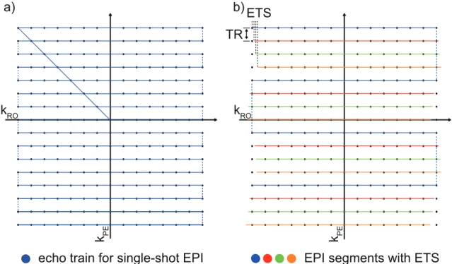
Figure 3.1: The sequence diagram for EPI acquisition shows the fast switching, alter-nating RO gradients and the gradient blips along PE following a slice selective excitation during FID. k-space data are sampled during the 64 readouts of the echo train. For illustration purposes the trapezoidal ramp up/down are not shown here.

Figure 3.2: a) Zig-zag traversal of k-space of a single-shot EPI. The trajectory moves forth and back along RO while blips shift it from line to line along PE. b) Segmentation of k-space into shorter echo trains allow a flexible timing and shortened TEs. The duration between EPI segments equals TR, i.e. acquisition of adjacent ky lines in the shown interleaved acquisition order. The meaning and benefit in SMS of the indicated phase modulation is described in Section 3.3.3 on CAIPIRINHA shifting.

3.1.2 Multi-Shot EPI

Typical limitations on spatial resolution, TE and distortions because of the long echo train in single-shot EPI can be addressed by segmentation of the echo train as illustrated in Figure 3.2. This type of acquisition scheme is known as segmented

(36)

or multi-shot EPI. The shorter echo-train length (ETL) yields less restrictions on resolution, possible values for TE and TR and reduces hardware demands. Even for signals with fast T₂∗-decay, multiple echoes can be acquired with segmented RO. Data of the individual segments are combined prior reconstruction into a complete k-space. Terminology differs in literature and sometimes regions of k-space divided up by each shot are called segments. However, here, a segment is formed by the zig-zag trajectory of the echo train after a RF excitation as shown in Figure 3.2. The flexibility of the readout requires longer overall scan time and, hence, an increased sensitivity to motion, which are the main drawbacks of multi-shot EPI compared to (single-shot) EPI. A long ETL accumulates off-resonance phase errors, which evolve continuously and map directly onto the k-space [FO94]. While the evolution of phase errors is reduced by shorter echo trains in multi-shot EPI, phase errors group together in adjacent segments and result in a stepwise phase discontinuities alongky at kx = 0. As shown in figure 3.2, slight temporal shifts of the successive echo trains, known as echo-time shifting (ETS), smoothen the k-space modulation function in the central k-space region and reduce image artifacts [FO94].

3.2 MRI with Multiple Receiver Coils

Phase manipulation by magnetic field gradients is one way to spatially encode the MR signal (Sec. 2.4). This is extensively employed in MR sequence design. Another way for spatial encoding is coil encoding [Bar+15]. The concept of coil encoding was presented theoretically by Hutchinson in 1988 [HR88] and first realized for imaging by Roemer in 1990 [REH90]. Since then, many accelerated acquisition techniques, e.g. parallel imaging (PI), omit time consuming gradient-based encoding steps, i.e. PE-encoding steps, and extract spatial information from the sensitivity patterns of the coil array [REH90; RR93]. Coil encoding then partially replaces PE encoding. The combination of both can also be considered as simultaneous encoding of several k-space data points. Furthermore, even if acceleration is not required, the detector’s proximity to magnetization in the region of interest and distance to disturbing magnetization and noise from the rest of the sample increase signal-to-noise ratio (SNR) compared to signal reception with a (single) body coil inside the scanner’s bore. In contrast to the advantages in SNR and encoding capability, multi coil arrays face additional challenges in their geometric design to balance local specificity and uniform (global) sensitivity.

The reception patterns of the individual coils form the so called coil sensitivity (CoS) profile. It describes the spatial B1 dependence of the coil array. Typical CoS profiles

of five representative coils in a 20-channel head coil are shown in Figure 3.3. The MR signal acquired with the individual coils after reconstruction (left) is compared

(37)

3.2 MRI with Multiple Receiver Coils to the images of identical slices after sum-of-squares (SoS) combination of all 20 coils (right). Variations in the signal intensities represent spatial receiver characteristics.

The SoS combination of the individual coil images results in a more homogeneous signal intensity.

Separate coil signal Combined

Sli ce 2 Sl ice 1

Figure 3.3: Two slices of a spherical phantom imaged with a 20-channels head coil (subset of five representative coils shown). a) The images of uncombined, individual coils show spatially discriminable, heterogeneous signal intensities contributing to the CoS profile. b) SoS coil combination gives a more homogeneous image of the object. For display purposes, theviridis colormap was used [Hun07] and colormap range was scaled differently for (a) and (b). A square-root mapping function was applied to account for the coil combination according to Equation 3.1 and to highlight local differences.

The SoS method to combine coil array signals or images is used throughout this work, because it has been shown that this simple but robust method approximates the theoretical upper bound if SNR is sufficiently high [Lar+03]. The signal contributions of all Nc individual coils, indexed with l, are combined by

S = ⌜ ⃓ ⃓ ⎷ Nc ∑︂ l=0 (Sl)2 (3.1)

to the final magnitude image.

The term coil is sometimes ambiguously used. A coil may refer to an individual coil element, but it commonly denotes the complete antenna unit as well, e.g. the head coil or the phased-array coil. In addition, the term channel is sometimes used synonymously for coil, although they can be differentiated technically. Channels are grouped coil elements in which signals are processed together to reduce the number of electronic components in the receiver chain [Els18]. This is mainly done for technical and financial reasons. The MR systems used for measurements in this work have separate circuitry for each coil and, therefore, the terms coil and channel are used interchangeably.

Sometimes PI as well as SMS are accounted as parallel imaging techniques since both utilize parallel or simultaneous signal acquisition from multiple coils and share similar reconstruction approaches. Therefore, the generalized autocalibrating

(38)

partially parallel acquisitions (GRAPPA) technique, which was first introduced for PI, will be described in Section 3.2.2, followed later on by modified GRAPPA-like methods to recover data which are undersampled along another dimension than PE.

3.2.1 Elimination of Noise Correlation in Coils

Multi coil arrays have an increased SNR compared to volume coils or large surface coils, because they can be placed in close proximity to the region of interest. Each individual detector response to signals from localized magnetization, but ignoring distant noise signal. However, the typically smaller diameter of the individual coils, with its reduced penetration depth, as well as interference between coils of the same coil array may have negative effects on the final SNR. The main source of image noise originates from the object to be imaged, because of its dielectric properties. Therefore, it is termed as (patient) loading or also called thermal or Johnson noise. In contrast, noise signal which is related to the electric circuitry is named electrical noise. Noise correlation occurs because coils receive partly identical thermal radiation if sensitivity regions of individual coils overlap [Pru+01]. Another source of signal correlation in coil arrays is the mutual induction between the coil elements. One can derive a noise covariance matrix from data of a noise-only measurement without RF excitation to determine the coupling of individual coils [Pru+01]. Typically, these calibration data to decorrelate coil signals are acquired once for a given configuration of object and coil array. Just like coil sensitivity, noise correlation between coils depends on coil positions and object and is assumed to be invariant over time. Coil arrays with a rigid structure, e.g. head coil, suffer less from noise correlation because of their optimized design and placement of the individual coils. However, if measurements are performed with flexible coil arrays or with a combination of coil arrays, noise decorrelation during signal processing is crucial as illustrated in Figure 3.4. The images show four slices of a pig’s hip and leg region taken with two 18-channels body coil arrays and eight coils of the spine coil array before perfusion experiments (Part II). The SNR appears significantly reduced for reconstructions without consideration of noise correlation (Fig. 3.4, left) compared to reconstructions with it (Fig. 3.4, right). This is because some coils in this configuration exhibit strong mutual coupling as shown in Figure 3.5 (a). The benefit of considering noise statistics scales with the encoding redundancy and is more pronounced the less equivalent the coils are to each other with respect to coil load, gain, coupling and electronic noise [Pru+01]. In practice, a change of basis from a set of real, physical coils to a set of virtual coils is realized where transformed coil data are decorrelated. The resulting reduction of the receiver’s noise-level increases final SNR. Therefore, a noise matrix Ψ of size Nc×Nc is determined experimentally by measuring samples in absence of a MR

signal. For statistical reasons about Nn = 103 noise samples per coil, arranged in a