White, S.R. and Kypraios, Theodore and Preston, Simon
P. (2015) Piecewise Approximate Bayesian
Computation: fast inference for discretely observed
Markov models using a factorised posterior distribution.
Statistics and Computing, 25 (2). pp. 289-301. ISSN
1573-1375
Access from the University of Nottingham repository:
http://eprints.nottingham.ac.uk/47125/1/10.1007%252Fs11222-013-9432-2.pdf
Copyright and reuse:
The Nottingham ePrints service makes this work by researchers of the University of
Nottingham available open access under the following conditions.
This article is made available under the Creative Commons Attribution licence and may be
reused according to the conditions of the licence. For more details see:
http://creativecommons.org/licenses/by/2.5/
A note on versions:
The version presented here may differ from the published version or from the version of
record. If you wish to cite this item you are advised to consult the publisher’s version. Please
see the repository url above for details on accessing the published version and note that
access may require a subscription.
DOI 10.1007/s11222-013-9432-2
Piecewise Approximate Bayesian Computation: fast inference
for discretely observed Markov models using a factorised
posterior distribution
S.R. White·T. Kypraios·S.P. Preston
Received: 17 December 2012 / Accepted: 24 October 2013 / Published online: 29 November 2013 © The Author(s) 2013. This article is published with open access at Springerlink.com
Abstract Many modern statistical applications involve in-ference for complicated stochastic models for which the likelihood function is difficult or even impossible to cal-culate, and hence conventional likelihood-based inferential techniques cannot be used. In such settings, Bayesian infer-ence can be performed using Approximate Bayesian Com-putation (ABC). However, in spite of many recent develop-ments to ABC methodology, in many applications the com-putational cost of ABC necessitates the choice of summary statistics and tolerances that can potentially severely bias the estimate of the posterior.
We propose a new “piecewise” ABC approach suitable for discretely observed Markov models that involves writing the posterior density of the parameters as a product of fac-tors, each a function of only a subset of the data, and then using ABC within each factor. The approach has the advan-tage of side-stepping the need to choose a summary statistic and it enables a stringent tolerance to be set, making the pos-terior “less approximate”. We investigate two methods for estimating the posterior density based on ABC samples for each of the factors: the first is to use a Gaussian approxima-tion for each factor, and the second is to use a kernel density estimate. Both methods have their merits. The Gaussian ap-proximation is simple, fast, and probably adequate for many
S.R. White (
B
)MRC Biostatistics Unit, Cambridge CB2 0SR, UK e-mail:[email protected] T. Kypraios·S.P. Preston
School of Mathematical Sciences, University of Nottingham, Nottingham NG7 2RD, UK
T. Kypraios
e-mail:[email protected] S.P. Preston
e-mail:[email protected]
applications. On the other hand, using instead a kernel den-sity estimate has the benefit of consistently estimating the true piecewise ABC posterior as the number of ABC sam-ples tends to infinity. We illustrate the piecewise ABC ap-proach with four examples; in each case, the apap-proach offers fast and accurate inference.
Keywords Approximate Bayesian Computation· Simulation·Stochastic Lotka–Volterra
1 Introduction
Stochastic models are commonly used to model processes in the physical sciences (Wilkinson 2011a; Van Kampen
2007). For many such models the likelihood is difficult or costly to compute making it infeasible to use conven-tional inference techniques such as maximum likelihood estimation. However, provided it is possible to simulate from a model, then “implicit” methods such as Approxi-mate Bayesian Computation (ABC) methods enable infer-ence without having to calculate the likelihood. These meth-ods were originally developed for applications in population genetics (Pritchard et al. 1999) and human demographics (Beaumont et al.2002), but are now being used in a wide range of fields including epidemiology (McKinley et al.
2009), evolution of species (Toni et al.2009), finance (Dean et al.2011), and evolution of pathogens (Gabriel et al.2010), to name a few.
Intuitively, ABC methods involve simulating data from the model using various parameter values and making in-ference based on which parameter values produced reali-sations that are “close” to the observed data. Let the data
x=(x1, . . . , xn)≡(x(t1), . . . , x(tn)) be a vector
Algorithm 1 Exact Bayesian Computation (EBC) 1: Sampleθ∗fromπ(θ ).
2: Simulate datasetx∗from the model using parametersθ∗. 3: Acceptθ∗ifx∗=x, otherwise reject.
4: Repeat.
Algorithm 2 Approximate Bayesian Computation (ABC) As Algorithm1, but with step 3 replaced by:
3’: Acceptθ∗ifd(s(x), s(x∗))≤ε, otherwise reject.
time pointst1, . . . , tn. We assume that the data arise from a
Markov stochastic model (which encompasses IID data as a special case) parameterised by the vectorθ, which is the target of inference, and we denote byπ(x|θ )the probabil-ity densprobabil-ity of the data given a specific value ofθ. Prior be-liefs aboutθare expressed via a density denotedπ(θ ). Algo-rithm1generates exact samples from the Bayesian posterior densityπ(θ|x)which is proportional toπ(x|θ )π(θ ).
This algorithm is only of practical use ifX(t )is discrete, else the acceptance probability in Step 3 is zero. For contin-uous distributions, or discrete ones in which the acceptance probability in step 3 is unacceptably low, Pritchard et al. (1999) suggested Algorithm 2, where d(·,·) is a distance function, usually taken to be theL2-norm of the difference between its arguments;s(·)is a function of the data; andε
is a tolerance. Note thats(·)can be the identity function but in practice, to give a tolerable acceptance rate, it is usually taken to be a lower-dimensional vector comprising summary statistics that characterise key aspects of the data.
The output of the ABC algorithm is a sample from the ABC posterior density π (θ˜ | x) = π(θ | d(s(x), s(x∗))≤ε). Provideds(·)is sufficient forθ, then the ABC posterior density converges to π(θ |x) as ε→0 (Marin et al.2012). However, in practice it is rarely possible to use ans(·)which is sufficient, or to takeεespecially small (or zero). Hence ABC requires a careful choice ofs(·)andεto make the acceptance rate tolerably large, at the same time as trying not to make the ABC posterior too different from the true posterior, π(θ|x). In other words, there is a balance which involves trading off Monte Carlo error with “ABC error” owing to the choice ofs(·)and toleranceε.
Over the last decade, a wide range of extensions to the original ABC algorithm have been developed, includ-ing Markov Chain Monte Carlo (MCMC) (Marjoram et al.
2003) and sequential (Toni et al. 2009; Dean and Singh
2011) implementations, the incorporation of auxiliary re-gression models (Beaumont et al.2002; Blum and François
2010), and (semi-)automatic choice of summary statistics (Fearnhead and Prangle2012); see Marin et al. (2012) for a review. In all of these ABC variants computational cost is still a central issue, since it is always the computational cost
that determines the balance that can be made between con-trolling Monte Carlo error and concon-trolling bias arising from using summary statistics and/or non-zero tolerance.
In this paper we propose a novel algorithm called
piece-wise ABC (PW-ABC), the aim of which is to substantially
reduce the computational cost of ABC. The algorithm is ap-plicable to a particular (but fairly broad) class of models, namely those with the Markov property and for which the state variable is observable at discrete time points. The algo-rithm is based on a factorisation of the posterior density such that each factor corresponds to only a subset of the data. The idea is to apply Algorithm2for each factor (a task which is computationally very cheap), to compute the density esti-mates for each factor, and then to estimate the full posterior density as the product of these factors. Taking advantage of the factorisation lowers the computational burden of ABC such that the choice of summary statistic and tolerance— and the accompanying biases—can potentially be avoided completely.
In the following section we describe PW-ABC in more detail. The main practical issue of the method is how to use the ABC samples from each posterior factor to estimate the full posterior density. We discuss two approaches to esti-mating the relevant densities and products of densities, then we apply PW-ABC, using both approaches, to four exam-ples: a toy illustrative example of inferring the probability of success in a binomial experiment, a stochastic-differential-equation model, an autoregressive time-series model, and a dynamical predator–prey model. We conclude with a dis-cussion of the strengths and limitations of PW-ABC, and of potential further generalisations.
2 Piece-wise ABC (PW-ABC)
Our starting point is to use the Markov property to write the likelihood as π(x|θ )= n i=2 π(xi|xi−1, . . . , x1, θ ) π(x1|θ ) = n i=2 π(xi|xi−1, θ ) π(x1|θ ). (1)
The likelihood contribution of the first data pointx1can be included in inference, but this contribution is asymptotically irrelevant as the number of observations,n, increases, and we henceforth follow the common practice to ignore the fac-torπ(x1|θ )in (1). Accounting for this, and by using mul-tiple applications of Bayes’ theorem, the posterior density can be written in the following factorised form,
Algorithm 3 Piece-Wise Approximate Bayesian Computa-tion (PW-ABC)
fori=2 tondo
a:Apply the ABC Algorithm to drawmapproximate (or exact, if s(·)=Identity(·) and ε =0) samples,
θi(∗1), . . . , θi(m)∗ , fromϕ˜i(θ ), the implied ABC density;
b: Using the samples θi(∗1), . . . , θi(m)∗ and either (6) or (12), calculate a density estimate,ϕˆi(θ ), ofϕ˜i(θ ).
end for
Substitute the density estimatesϕˆi(θ )into (3) to calculate
an estimate,π (θˆ |x), ofπ(θ|x). π(θ|x)∝π(x|θ )π(θ ) = n i=2 π(xi|xi−1, θ )π(θ ) π(θ ) π(θ ) ∝π(θ )(2−n) n i=2 ϕi(θ ) , (2) where ϕi(θ )=ci−1π(xi|xi−1, θ )π(θ ) ci= π(xi|xi−1, θ )π(θ )dθ.
Essentially, in (2) the posterior density,π(θ|x), ofθgiven the full dataxhas been decomposed into a product involving densitiesϕi(θ ), each of which depends only on a pair of data
points,{xi−1, xi}.
The key idea now is to use ABC to draw approximate samples from each of the densitiesϕi(θ ). Applying
Algo-rithm 2involves (i) drawingθ∗ from π(θ ), (ii) simulating
xi∗|xi−1, θ∗, and (iii) acceptingθ∗ if d(s(xi), s(xi∗))≤ε.
We use ϕ˜i(θ ) to denote the implied ABC density from
which these samples are drawn (withϕ˜i(θ )=ϕi(θ )ifs(·)=
Identity(·) andε=0). By repeating (i)—(iii) we generate samples of, say,mdraws,θi(∗1), . . . , θi(m)∗ , from eachϕ˜i(θ ).
Now, suppose thatϕˆi(θ )is an estimate, based on the sample
θi(∗1), . . . , θi(m)∗ , of the densityϕ˜i(θ )(and hence of the
den-sityϕi(θ )). Then the posterior density (2) can be estimated
by ˆ π (θ|x)=g(θ ) g(θ )dθ, (3) where g(θ )=π(θ )(2−n) n i=2 ˆ ϕi(θ ) . (4)
The steps of PW-ABC are summarised in Algorithm3. The rationale of the piecewise approach is to reduce the dimension for ABC, replacing a high-dimensional problem
with multiple low-dimensional ones. In standard ABC the summary statistic,s(·), is the tool used to reduce the dimen-sion, but in PW-ABC, with dimension already reduced by the factorisation in (2), we can takes(·)=Identity(·)and typically use a much smallerε.
The question remains of how to calculate the density es-timates,ϕˆi(θ ). Below we discuss two approaches: (i) using
a Gaussian approximation, and (ii) using a kernel density estimate. Henceforth, quantities based on (i) are denoted by superscript g, and those based on (ii) are denoted by super-script k. In both cases we discuss the behaviour of the es-timators in the asymptotic regime in which the number of observations,n, is kept fixed while the size of each ABC sample increases,m→ ∞.
2.1 Gaussian approximation forϕˆi(θ )
Denote the d-dimensional multivariate Gaussian density with mean,μ, and covariance,Σ, by
K(θ;μ, Σ )=(2π )−d/2(detΣ )−1/2 ×exp −1 2(θ−μ) TΣ−1(θ−μ) . (5) A Gaussian approximation forϕˆi(θ )is
ˆ ϕig(θ )=K θ; ¯θi∗, Qi , (6) where ¯ θi∗= 1 m m j=1 θi(j )∗ , Qi = 1 m−1 m j=1 θi(j )∗ − ¯θi∗ θi(j )∗ − ¯θi∗T,
are the sample mean and sample covariance of the ABC pos-terior sampleθi(∗1), . . . , θi(m)∗ . A consequence of using (6) is that the product of the density approximations is also Gaus-sian (though in general unnormalised):
n i=2 ˆ ϕig(θ )=w·K(θ;a, B), (7) where B= n i=2 Q−i 1 −1 , (8) a=B n i=2 Q−i 1θ¯i∗ , (9) w=det(2π B)1/2 n i=2 det(2π Qi)−1/2
× n s=2 n t >s exp −1 2 θ¯ ∗ s − ¯θt∗ T Rst θ¯s∗− ¯θt∗ , (10) Rst=Q−s1BQ−t 1. (11)
We note the following properties of approximation (6) (see, for example, Mardia et al. 1979). If the densities ϕ˜i(θ )
from which theθi(∗1), . . . , θi(m)∗ are drawn are Gaussian, i.e., ˜
ϕi(θ )=K(θ;μi, Σi), thenθ¯i∗andQiare unbiased and
con-sistent estimators ofμi andΣi, respectively, and hencea
and B are consistent estimators of the true mean and co-variance ofϕ˜i(θ ). More generally, forϕ˜i(θ )which is not
necessarily Gaussian, θ¯i∗ andQi are consistent estimators
of the mean and the variance of the Gaussian density,ϕˆig(θ ), which minimises the Kullback–Leibler divergence,
KL ϕ˜i(θ ) ˆϕgi(θ ) = ˜ ϕi(θ )log ϕ˜i(θ )/ϕˆig(θ ) dθ;
i.e., for eachi,ϕˆgi(θ )is asymptotically the “optimal” Gaus-sian approximation to ϕ˜i(θ ). No such relevant optimality
holds for the product of densities, however: the (normalised) product of Gaussians, each of which is closest in the KL sense toϕ˜i(θ ), is in general not the Gaussian closest to (the
normalised version of)ϕ˜i(θ ); and indeed it may be very
substantially different. In other words, asm→ ∞,aandB
do not in general minimise
KLϕ˜i(θ )/ ϕ˜i(θ )K(θ, a, B)
.
2.2 Kernel density estimate forϕˆi(θ )
A second method we consider is to estimate each density ˜
ϕi(θ )using a kernel density estimate (see for instance
Sil-verman1986and Wand and Jones1995). A kernel density estimate based on Gaussian kernel functions (5) is
ˆ ϕki(θ )= 1 m m j=1 K θ;θi(j )∗ , Hi , (12)
whereHi is a bandwidth matrix. We follow the approach
of Fukunaga (1972) in choosing the bandwidth matrix such that the shape of the kernel mimics the shape of the sample, in particular by taking Hi to be proportional to the sample
covariance matrix,Qi. Using bandwidth matrix
Hi=q·m−2/(d+4)Qi, (13)
whereq >0 is a constant not dependent onm, ensures de-sirable behaviour as the sample sizem→ ∞. In particular, in terms of the little-o notation (am=o(bm)asm→ ∞
de-notes limm→∞|am/bm| =0) and withEdenoting
expecta-tion, using choice of bandwidth (13), subject to mild regu-larity conditions onϕ˜i(θ )(Wand and Jones1995),
Eϕˆik(θ )= ˜ϕi(θ )+o(1), (14)
Eϕˆik(θ )2= ˜ϕi(θ )2+o(1). (15)
From (14)–(15), the bias, b{ ˆϕki(θ )} =E{ ˆϕki(θ )} − ˜ϕi(θ ),
the variance, var{ ˆϕik(θ )} =E{ ˆϕik(θ )2} −E{ ˆϕik(θ )}2, and the mean integrated squared error,
MISEϕˆik=E ϕˆik(θ )− ˜ϕi(θ )
2
dθ, (16)
are allo(1). These results generalise routinely to the case of a product ofnkernel density estimates, that is, in which
ˆ
ϕik(θ )is used as an estimator forϕ˜i(θ ). It follows that
since theθi(j )∗ are independent for alli, j, then, using (14)– (15), bϕˆik(θ ) =Eϕˆik(θ ) −ϕ˜i(θ )=o(1), varϕˆik(θ ) =Eϕˆki(θ )2−Eϕˆik(θ )2=o(1), MISEϕˆik =E ϕˆik(θ )−ϕ˜i(θ ) 2 dθ=o(1).
Hence, in the sense defined by the latter equation, the density estimatorϕˆik(θ )converges to the true densityϕ˜i(θ )as
m→ ∞.
Regarding the choice ofqin (13), in certain settings it is possible to determine an optimal value. Suppose that the true densityϕ˜i(θ )is Gaussian and letϕˆik(θ )in (12) be a kernel
density estimate ofϕ˜i(θ ). Then
q=(d+2)/4−2/(d+4) (17) is optimal in the sense that (13) is then an unbiased and con-sistent estimator of the bandwidth that minimises the leading term of the large-masymptotic expansion of (16); see Wand and Jones (1995, p. 111). Analogous calculations are rather more involved in the product case, however: even with the assumption that eachϕ˜i(θ )is Gaussian, no closed
expres-sion forqis possible. Hence, in the examples in the follow-ing section, Sect.4, we opted to tuneq in the heuristic way described by Wand and Jones (1995), starting with a largeq
(ten times that in (17)) then reducing it manually until “ran-dom” fluctuations begin to appear in the density estimates.
A consequence of using Gaussian kernel functions (5) in (12) is that the product of the density approximations is then itself a weighted mixture of(n−1)mGaussians,
n i=2 ˆ ϕik(θ )=m(1−n) n i=2 m j=1 K θ;θi(j )∗ , Hi =m(1−n) m j2,...,jn n i=2 K θ;θi(j∗ i), Hi = m j2,...,jn wj2,...,jnK(θ;aj2,...,jn, Bj2,...,jn), (18)
where expressions for the covariances Bj2,...,jn, means
aj2,...,jn, and weights wj2,...,jn, analogous to those in (8)– (10), are given in Appendix1.
2.3 Estimating the posterior density
Sections 2.1and 2.2 describe methods for computing the factor ϕˆi(θ ) in (3). For calculating an estimate of the
full posterior,π (θˆ |x)in (3), we must multiplyϕˆi(θ )by
π(θ )(2−n) and normalise. Let us suppose that the prior is Gaussian,π(θ )=K(θ;μpri, Σpri). For the case where we are using the Gaussian approximation,ϕˆig(θ ) from (6), for eachϕˆi(θ ), then the posterior is
ˆ πg(θ|x)=K(θ;μpost, Σpost), (19) where Σpost= (2−n)Σpri−1+B− 1−1 , (20)
μpost=Σpost (2−n)Σpri−1μpri+B−1a
, (21)
andaandBare as defined in (7).
If instead we use the kernel approximation, ϕˆik(θ )
from (12), for eachϕˆi(θ ), then the posterior density is
ˆ πk(θ|x)= m j2,...,jn wj 2,...,jnK θ;aj2,...,jn, Bj2,...,jn m j2,...,jn wj 2,...,jn, (22)
where expressions forBj
2,...,jn,aj2,...,jn andwj2,...,jn are in Appendix1.
2.4 An expression for the posterior density
In the preceding sections we considered how to sample from theϕi(θ )and then use the samples to estimate the posterior
density π(θ |x). Here we consider in more detail the im-plied posterior density which is targeted by PW-ABC. For either of PW-ABC and ABC, the posterior can be written as
˜
π (θ|x)∝ ˜π (x|θ )π(θ ), (23) whereπ (x˜ |θ )is, respectively, either the implied PW-ABC or ABC approximation to the likelihood. First, we define the function
Kε,p(z)=V−11{zp≤ε}, (24)
where argument z is of dimension, say, u, and either continuous- or discrete-valued in accord with the support of the data; · pis theLp-norm;1{·}is an indicator
func-tion; and V, which depends onu, ε, and p, is such that
Kε,p(z)dz=1, with this integral interpreted as a sum in
the discrete case. For ABC with distanced(·,·)taken to be the Lp-norm of the difference between its arguments, the implied ABC approximation to the likelihood (Wilkinson
2013) is the convolution
˜
πABC(x|θ )=
π(y|θ )Kε,p(y−x)dy. (25)
Hence ABC replaces the true likelihood with an approxi-mate version averaged over anLp-ball of radiusεcentred on the data vector,x. In PW-ABC, we target eachϕi(θ )by an
ABC approximationϕ˜i(θ )∝ ˜πABC(xi|xi−1, θ )π(θ ), with ˜
πABC(xi|xi−1, θ )=
π(yi|xi−1, θ )Kε,p(yi−xi)dyi,
and the implied PW-ABC likelihood is the product ˜
πPW-ABC(x|θ )=
˜
πABC(xi|xi−1, θ ). (26) Now, to compare directly the implied ABC and PW-ABC likelihood approximations, we neglect as before the likeli-hood contribution from the first observationx1, then denote byx the vectorxwithx1removed (and similar fory); hence we can write (25) and (26), respectively, as
π(y2|x1, θ ) n i=3 π(yi|yi−1, θ ) Kε,p y −x dy, (27) and π(y2|x1, θ ) n i=3 π(yi|xi−1, θ ) Kε,p∗ y −x dy, (28) where Kε,p∗ z= n i=2 Kε,p zi . (29)
Two differences between ABC and PW-ABC are clear: first, in ABC the conditioning is on the simulated trajectory, whereas in PW-ABC the conditioning is on the data; and second, in PW-ABC the convolution is with respect to a dif-ferent kernel (29). This implied kernel seems intuitively rea-sonable; for example, if thexi are scalar then the
convolu-tion in (28) amounts to an averaging over a hypercube of side length 2εcentred onx . The difference in the shapes of the regions defined byKε,p(·)andKε,p∗ (·)is of secondary
importance, however, since PW-ABC enables use of a much smallerεthan ABC, so the averaging will be over a much smaller region around x, and the approximate likelihood will typically be much closer to the true.
3 Some other considerations
3.1 Practical issues in drawing samples
The independence of the samplesθi(j )∗ for alli, jmeans that drawing samples for PW-ABC is “embarrassingly parallel”, i.e., the task can be divided easily between multiple cores. For example, one approach is use all available cores simul-taneously to sample fromϕ˜2(θ )untilmdrawsθ2∗(1)· · ·θ2∗(m) are accepted, and then do likewise forϕ˜3(θ ), and so on. An-other possibility, which requires less coordination between the cores, is to have different cores sampling from differ-entϕ˜i(θ ), then reassign cores as appropriate whenever any
of theϕ˜i(θ )reachesmaccepted samples.
Another benefit of the θi(j )∗ being independent is that samples can be reused in the event of deciding retrospec-tively to perform PW-ABC with a smallerε: the subset of original samples acceptable with the new smallerε can be retained, leaving only the need, for eachϕ˜i(θ ), to “top-up”
the number of samples to m. Similarly, samples can ob-viously be retained given a retrospective decision to use a largerm.
3.2 Estimating the marginal likelihood
In some applications, especially when model comparison is of interest, it is useful to compute the marginal likelihood of the data given the model. The marginal likelihood is
π(x)= π(x|θ )π(θ )dθ (30) = n i=2 ci n i=2 ϕi(θ ) π(θ )2−ndθ. (31)
The unknownci can be estimated bycˆi=m/(V Mi), where
Mi equals the number of ABC draws necessary in theith
interval to achievemacceptances, andV is defined in (24); see Appendix2. For the integral in (31), using the Gaussian approximation (7) leads to n i=2 ˆ ϕig(θ ) π(θ )2−ndθ
=w·(detB)−1/2·(detΣpost)1/2· det(2π Σpri) (n/2−1) ×exp −1 2(a−μpri) T ( 2−n)−1Σpri+B −1 ×(a−μpri) , (32)
whereas using the kernel approximation (12) gives
n i=2 ˆ ϕik(θ ) π(θ )2−ndθ= m j2,...,jn wj 2,...,jn. (33)
3.3 Practical numerical calculations for the kernel approximation
Since expressions (18), (22), (33) for the kernel case involve sums with(n−1)mterms, these expressions are largely of academic interest and are typically not suitable for practical calculations. For the examples in this paper we used a more direct numerical approach, first writing (4) as
g(θ )=exp n i=2 hi(θ ) π(θ ),
wherehi(θ )=log(ϕik(θ )/π(θ )), and then evaluatinghi(θ ),
π(θ )and henceg(θ )pointwise on a fine lattice. Performing calculations in this way on the log scale avoids underflow er-rors and improves numerical stability compared with trying to evaluate (4) directly. As a further check for robustness, we varied the lattice position and resolution to make sure the results were insensitive to the particular choices. 3.4 Sampling from the posterior distribution
In some circumstances it may be desirable to draw sam-ples from the approximate posterior density. In the Gaussian case, drawing from (19) is straightforward. For the kernel case, (22), in principle sampling can be achieved by nor-malising the weights, randomly choosing a component with probability equal to these normalised weights, then sam-pling from the selected Gaussian component. But in prac-tice, again, the large number of terms in (22) will typically preclude this approach. Other possibilities include using a Gibbs sampler, or sampling approximately using Gaussian mixtures with fewer components; see Sudderth et al. (2003).
4 Examples
In this section we test PW-ABC on synthetic data from four models. The first, as a toy illustrative example, involves in-ferring from IID data the probability of success in a bino-mial experiment. Second is the Cox–Ingersoll–Ross model, a stochastic-differential-equation model for which the con-tinuous state variable has known transition density, which we use to investigate PW-ABC withε >0. Third, we con-sider an integer-valued time series model called INAR(1), a model for which the likelihood is available (albeit awk-ward to compute) and enables comparison of our approach with a “gold standard” MCMC approach. Finally, we con-sider a stochastic Lotka–Volterra model, a simple example from a common class of models (which occur, for instance, in modelling stochastic chemical kinetics) in which the like-lihood, and therefore many standard methods of inference, are unavailable.
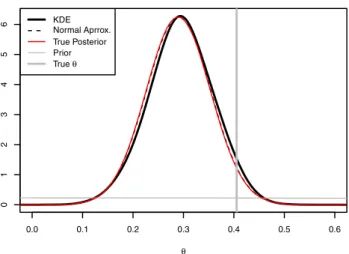
Fig. 1 Results for the binomial model in Sect.4.1. Shown are the true posterior density,π(θ|x), the posterior density approximations
ˆ
πg(θ|x)andπˆk(θ|x), the prior, and the trueθ
4.1 Binomial model
For this toy example we suppose the data is the set x =
{x1, . . . , x10}of n=10 observations from the modelXi ∼
Binom(ki =100, p=0.6). We work in terms of the
trans-formed parameter θ = logit(p), using a prior π(θ ) ∼ N (0,32). For this model the data are IID, so that
π(xi | xi−1, θ ) = π(xi | θ ). Exact samples from ϕi(θ )
can be obtained by sampling θ∗ from the prior, sampling
X∗i ∼Binom(100, θ∗), and then accepting θ∗ if and only ifX∗i =xi. We follow the PW-ABC approach described in
Sect. 2, drawing m=5000 samples from each ϕi(θ ),
us-ing these samples to construct Gaussian ϕˆig(θ ) and kernel densityϕˆik(θ )approximations, then using these density ap-proximations to construct approximate posterior densities,
ˆ
πg(θ |x)and πˆk(θ |x). Figure 1 shows that the approx-imate posterior densities are very close to the true poste-rior density for this example. The true log marginal likeli-hood, logπ(x), computed by direct numerical integration of (30), is −31.39; using approximation ϕˆgi(θ ) and (32) gives−31.44; and using approximationϕˆik(θ )and numeri-cal integration of the left-hand side of (33) gives−31.48. 4.2 Cox–Ingersoll–Ross Model
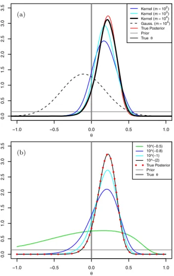
The Cox–Ingersoll–Ross (CIR) model (Cox et al.1985) is a stochastic differential equation (SDE) describing evolution of an interest rate,X(t ). The model is
dX(t )=a b−X(t )dt+σX(t )dW (t ),
wherea,bandσrespectively determine the reversion speed, long-run value and volatility, and where W (t ) denotes a standard Brownian motion. The density ofX(ti)|X(tj),a,
b,σ (ti> tj) is a non-central chi-square (Eq. (18), Cox et al.
1985), and hence the likelihood is known in closed form. Since the likelihood is known, (PW-)ABC is unnecessary (indeed, in general for SDEs with unknown likelihoods, ap-proaches that exploit the SDE structure—e.g., the likelihood approximations of Aït-Sahalia (2002), or the Monte Carlo methods developed by Durham and Gallant (2002)—are likely to be better choices for inference than (PW-)ABC); however, we include the CIR model here as a simple exam-ple of PW-ABC applied to a problem with a continuous state variable, where non-zero choice ofεis necessary, and where the true posterior distribution is available for comparison.
We generatedn=10 equally spaced observations from a CIR process with parameters(a, b, σ )=(0.5,1,0.15)and
X(0)=1 on the interval t∈ [0,4.5]. Treating a andσ as known, we performed inference on the transformed parame-terθ=log(b)with a Uniform prior on the interval(−5,2). Usingε=10−2we drew samples of size m=10,000 for eachϕi(θ ),i=2, . . . ,10, achieving acceptance rates around
1.5 % on average.
Figure2(a) shows the true posterior density,π(θ |X), together with the Gaussian- and kernel-based PW-ABC ap-proximations,πˆg(θ|x)andπˆk(θ|x). The figure shows that for sufficiently largemthe kernel approximationπˆk(θ|x)
agrees very well with the true posterior. The Gaussian ap-proximationπˆg(θ |x), even for large m, does badly here, which is due to skewness of the densitiesϕi(θ ). Figure2(b)
shows how the posterior density targeted by PW-ABC (see Sect.2.4) depends onε, and in particular how it converges to the true posterior density asε→0.
For this example, estimates of the log marginal likeli-hood, logπ(X)are as follows: by direct numerical integra-tion of (30), 8.14; using approximationϕˆig(θ ), 2.78; and by usingϕˆik(θ )in conjunction with numerical integration of the left-hand side of (33), 7.93.
4.3 An integer-valued autoregressive model
Integer-valued time series arise in contexts such as mod-elling monthly traffic fatalities (Neal and Subba Rao2007) or the number of patients in a hospital at a sequence of time points (Moriña et al.2011). Consider the following integer-valued autoregressive model of orderp, known as INAR(p):
Xt= p
i=1
αi◦Xt−i+Zt, t∈Z, (34)
where Zt for t >1 are independent and identically
dis-tributed integer-valued random variables withE[Zt2]<∞,
with theZt assumed to be independent of theXt. Here we
assume Zt ∼P o(λ). Each operator αi◦ denotes binomial
thinning defined by
αi◦W=
Binomial(W, αi), W >0,
Fig. 2 Results for the CIR model of Sect.4.2. (a) shows the true pos-terior density,π(θ|x); the PW-ABC posterior density approximations
ˆ
πg(θ|x)andπˆk(θ|x)usingε=10−2, with values ofmindicated in the legend; the prior; and the trueθ. (b) shows, for various values ofε, the true PW-ABC posterior (defined in Sect.2.4)
for non-negative integer-valued random variableW. The op-eratorsαi◦,i=1, . . . p, are assumed to be independent.
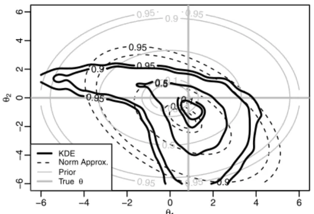
We consider the simplest example of this model, INAR(1) (see, for example, Al-Osh and Alzaid1987), supposing that we have some observed data x = {x1, . . . , xn} from this
model and wish to make inference for the parameters(α, λ). We generatedn=100 observations from an INAR(1) pro-cess using parameters(α, λ)=(0.7,1)andX(0)=10; the realisation is plotted in Fig. 3. Working in terms of the transformed parameter, θ =(θ1, θ2)=(logit(α),log(λ)), we used a prior of Norm(0,32)for each ofθ1andθ2. For the EBC algorithm, the probability of acceptance is around 10−100(as estimated from PW-ABC calculations described below), which is prohibitively small; even the ABC algo-rithm requires a value of ε so large that sequential ap-proaches are needed.
Fig. 3 The realisation of an INAR(1) process used in the example of Sect.4.3, of lengthn=100, generated usingα=0.7 andλ=1.0
Fig. 4 Results for the INAR(1) example of Sect.4.3. Shown are an MCMC approximation to the posterior density,π(θ|x), the poste-rior density approximationsπˆg(θ|x)andπˆk(θ|x), the prior, and the trueθ. The numbers on the contours denote the probability mass that they contain
Using PW-ABC with ε=0 we were able to draw ex-act samples from ϕi(θ ) for all of the i=2, . . . ,100
fac-tors, and achieve acceptance rates of around 9 %, on av-erage. Figure4shows an estimate of the posterior density,
π(θ |x) based on a gold-standard MCMC approach, to-gether with Gaussian- and kernel-based PW-ABC approx-imations, πˆg(θ |x)andπˆk(θ |x), with m=10,000 sam-ples for eachϕi(θ ). The figure shows good agreement
be-tween the MCMC posterior and the kernel approximation, ˆ
πk(θ |x), but again somewhat poor agreement with the Gaussian approximationπˆg(θ|x). The poor performance of
ˆ
πg(θ|x)is caused by some of the densitiesϕi(θ )being
sub-stantially different from Gaussian; see Fig.5 which shows ˆ
ϕ50g(θ ) and ϕˆ50k(θ ), for example. Using Gaussian approxi-mations to non-Gaussianϕi(θ )appears to have a strong
im-pact on the accuracy of approximationπˆg(θ|x), even, as in the present case, where the true posteriorπ(θ|x), and most of individualϕi(θ ), are reasonably close to a Gaussian (cf.
Fig.4).
For this example, estimates of the log marginal likeli-hood, logπ(x), are as follows: by direct numerical
integra-Fig. 5 For the INAR(1) example, an example of a factor with a “non– Gaussian” density: hereϕˆ50g(θ )andϕˆ50k(θ )are substantially different from each other
tion of (30),−161.1; using approximationϕˆig(θ )and (32), −185.7; and by using ϕˆik(θ ) and numerical integration of the left-hand side of (33),−163.2.
We have used p=1 for this example so that the like-lihood is available, enabling comparison with MCMC and calculation of the true marginal likelihood. However, we stress that PW-ABC can be easily generalised for p >1, a case for which the likelihood is essentially intractable and therefore one has to resort to either exact but less direct methods (such the Expectation–Maximization (EM) algorithm or data-augmented MCMC, both of which in-volve treating the terms αi ◦Xt−i andZt as missing data)
or methods of approximate inference, such as conditional least squares which involves minimizing t(Xt −E[Xt |
Xt−1])2; see, for example, McKenzie (2003) and references therein.
4.4 Stochastic Lotka–Volterra model
The stochastic Lotka–Volterra (LV) model is a model of predator–prey dynamics and an example of a stochastic discrete-state-space continuous-time Markov process (see, for example, Wilkinson 2011a). Predator–prey dynamics can be thought of in chemical kinetics terms: the predators and prey are two populations of “reactants” subject to three “reactions”, namely prey birth, predation and predator death. Exact simulation of such models is straightforward, e.g., us-ing the algorithm of Gillespie (1977). Inference is simple if the type and precise time of each reaction is observed. However, a more common setting is where the population sizes are only observed at discrete time points. In this case the number of reactions that have taken place is unknown and therefore the likelihood is not available and hence in-ference is much more difficult. Reversible-jump MCMC has been developed in this context (Boys et al.2008) but it re-quires substantial expertise and input from the user to imple-ment. Particle MCMC (pMCMC) methods (Andrieu et al.
2010), which provide an approximation to the likelihood via a Sequential Monte Carlo algorithm within an MCMC al-gorithm, have recently been proposed for stochastic chem-ical kinetics models (Golightly and Wilkinson2011). Al-though being computationally intensive, such methods can work reliably provided the process is observed with mea-surement error. TheRpackagesmfsb, which accompanies (Wilkinson2011a), contains a pMCMC implementation de-signed for stochastic chemical kinetics models, and we use this package to compare results for PW-ABC and pMCMC for the following example.
LetY1andY2 denote the number of prey and predators respectively, and supposeY1 andY2are subject to the fol-lowing reactions Y1 r1 →2Y1, Y1+Y2 r2 →2Y2, Y2 r3 → ∅, (36) which respectively represent prey birth, predation and predator death. We consider the problem of making infer-ence about the rates(r1, r2, r3)based on observations ofY1 andY2made at fixed intervals.
We generated a realisation from the stochastic LV exam-ple of Wilkinson (Wilkinson, p. 208), that is, model (36) using(r1, r2, r3)=(1,0.005,0.6),Y1(0)=50 andY2(0)= 100. We performed inference in terms of transformed parameters, θ = (θ1, θ2, θ3) =(logr1,logr2,logr3), this time with priors π(θ1) ∼Norm(log(0.7),0.5), π(θ2)∼ Norm(log(0.005),0.5), and π(θ3)∼Norm(log(0.3),0.5). We again applied PW-ABC usingε=0, in other words re-quiring an exact match between the observed and the simu-lated observations, to draw samples of sizem=10,000 for eachϕi(θ ). Unlike the binomial, CIR and INAR examples
where drawing posterior samples for theϕi(θ ),i=1, . . . , n
assuming=0 took a total of approximately, 1, 2 and 20 minutes respectively on a standard desktop machine, for this example doing so was computationally more demanding. However, since sampling in PW-ABC is embarrassingly par-allel (see Sect.3.1) we were able to draw the required sam-ples in 32 hours on a 48 core machine.
To obtain pMCMC results we found it necessary to as-sume an error model for the observations, hence we asas-sumed errors to be IID Gaussian with mean zero and standard devi-ation equal to 2. Results are displayed in Fig.6, which shows plots for univariate and pairwise bivariate marginal posterior densities for the pMCMC results, and for the PW-ABC ap-proximations,πˆg(θ|x)andπˆk(θ|x). Both of the PW-ABC approximations agree well with each other and with the pM-CMC results for this example.
5 Conclusion and discussion
PW-ABC works by factorising the posterior density, for which targeting by ABC would entail a careful choice ofs(·)
Fig. 6 Results for the Lotka–Volterra example of Sect.4.4, showing univariate and bivariate marginal posterior densities ofθbased on a posterior sample from a pMCMC algorithm, and from the Gaussian- and kernel-based PW-ABC approximations,
ˆ
πg(θ|x)andπˆk(θ|x). For the kernel approximation we used q=5 as the smoothing parameter in (13). The contours shown in the bivariate plots are those that contain 5 %, 10 %, 50 %, 90 % and 95 % of probability mass
and/or a large tolerance ε, into a product involving densi-tiesϕi(θ ), each amenable to using ABC withs=Identity(·)
and small or zero ε. Having sampled from eachϕi(θ ) the
question then becomes how to estimateπ(θ|x)using these samples. In PW-ABC, we construct density estimatesϕˆi(θ )
of eachϕi(θ )then approximateπ(θ|x)as the product of
the ϕˆi(θ ). The approach of taking ϕˆi(θ ) to be Gaussian,
with moments matched to the sample moments, is computa-tionally cheap, and if the prior is also taken to be Gaussian then there is a closed form expression for the Gaussian pos-terior density and marginal likelihood, making calculations extremely fast. Takingϕˆi(θ )to be Gaussian is perhaps
ade-quate in many applications: performance was strong in two of the four examples we considered. The poor performance in the CIR and INAR examples was due to skewness of at least some of theϕi(θ ). In the INAR example it is striking to
see an effect so strong when the true posterior, and many of theϕi(θ ), are so close to Gaussian. Unfortunately,
increas-ing the number, m, of ABC samples is no remedy to this problem: as m→ ∞, the normalised product of Gaussian
densities, itself Gaussian, in general does not converge to the Gaussian density closest in the Kullback–Leibler sense to the target density.
Two referees suggested the possibility of testing, across all of theϕi(θ ), whether a Gaussian approximation is
appro-priate. A wide literature exists on testing multivariate nor-mality (see Székely and Rizzo2005for a recent contribu-tion, plus many references therein to earlier work) and this seems a promising direction, but further work is needed to devise, and understand the properties of, a procedure based on applying these tests in the multi-testing setting of PW-ABC.
In terms of asymptotic performance, using the kernel ap-proximation, ϕˆik(θ ), for ϕˆi(θ ) is preferable since, in this
case, the estimated posterior density converges to the target as m→ ∞. The kernel approach is computationally more
demanding, however, and its practical use is probably lim-ited to problems in whichθ has small dimension. It also requires a heuristic choice of a scalar smoothing parameter. The larger the value chosen for the smoothing parameter, the
more the posterior variance will be inflated; this said, how-ever, in the examples we have considered we have found posterior inference to be fairly robust to the choice. A ref-eree asked for guidance on how to choosem. It is difficult to offer general practical advice, because themneeded will depend on the dimension ofθ, and on the number and nature of the ϕi(θ ). The larger the better, of course; one
possibil-ity for checking whethermis large enough might be to use a resampling approach to confirm that the variance, under resampling, of theπˆk(θ|x)is acceptably small.
Another related practical question is how to choose ε
if ε=0 is not possible. In such a case, as with standard ABC approaches, there is a trade-off between making m
large and makingεsmall. A reasonable heuristic to inves-tigate the effects of non-zero ε would be to perform in-ference with a chosen ε andm, and then to keep mfixed and reduceε(as discussed in Sect.3.1, acceptable samples from the run with largerεcan be retained), and then check whether there is a marked difference in the posteriors for the different values ofε. Figure2(b) shows for the CIR ex-ample, for instance, that there would be little difference be-tween the posteriors forε=10−2andε=10−3. Such an ap-proach could be applied iteratively, although for challenging problems—even using PW-ABC—the computational cost to maintain msamples as ε is decreased may prevent reach-ing a small enough εthat the posterior has “converged” to the true. Such a heuristic could be applied to standard ABC, of course, although PW-ABC has the advantage of enabling much smaller choices ofε.
The underlying idea in PW-ABC of replacing a high-dimensional ABC problem with multiple low-high-dimensional ones is also exploited in some sequential ABC algorithms; for example, Algorithm 4 in Fearnhead and Prangle (2012) (adapted from an algorithm by Wilkinson2011b) uses ABC to incorporate observations from a Markov model sequen-tially, the ABC at each step involving a single data point con-ditional on the previous one, and where the posterior from one step is used as the prior for the next. In comparison with PW-ABC, such sequential algorithms have a potential ad-vantage of progressively focusing computational effort on regions of parameter space with high posterior density, but on the other hand they are prone to problems with particle degeneracy, an issue that does not affect PW-ABC. Another major difference is that for sequential algorithms, samples at each step are dependent, so calculations are not “embar-rasingly parallel”, and nor is it so easy to reuse samples in the event of a retrospective decision to use a smaller ε or largerm; see Sect.3.1.
A possibility that generalises the Gaussian and kernel ap-proaches in PW-ABC, which we will explore in future work, is to letϕˆi(θ ) be a mixture of, say, u Gaussians (see Fan
et al.2012for an example of Gaussian mixtures being used in a related context). This encompasses (6) and (12) as spe-cial cases, withu=1 andu=mrespectively. For a general
mixture model forϕˆi(θ ), each of the component Gaussians
is parameterised by a scalar weight, a mean vector and a covariance matrix which need to be determined. We would envisage regularising, e.g., by setting each covariance to be equal up to scalar multiplication, perhaps as for (12) tak-ing the covariance proportional to the sample covariance, and then fitting eachϕˆi(θ )based on the samples fromϕi(θ )
using, say, an EM algorithm. This approach is a compro-mise between (6) and (12). It does not share the property of (12) that estimated densities converge to the true densi-ties asm→ ∞, but on the other hand it is computationally
much less involved and offers much extra freedom and flexi-bility over (6), particularly for dealing with multimodal den-sities. Ifuis taken sufficiently small then it may be feasible to work explicitly with the (n−1)u-term resulting Gaus-sian mixture,ϕˆi(θ ), enabling explicit calculations
involv-ing the posterior density, such as computinvolv-ing the marginal likelihood, analogous to (32), and direct sampling from the approximate posterior density (see Sect.3.4).
Several further generalisations of PW-ABC are pos-sible. In (1), each of the n−1 factors π(xi |xi−1, θ ),
i=2, . . . , n is the likelihood for a single data point con-ditional on the previous. An alternative possibility is to factorise the likelihood into fewer factors, with each cor-responding to a “block” of multiple observations, e.g.,
π(xi+vi, xi+vi−1, . . . , xi |xi−1, θ ) for some choice of vi, and the factorised likelihood becomes a product over the relevant subset ofi=2, . . . , n. To an extent this potentially reintroduces difficulties that with PW-ABC we sought to avoid, namely lower acceptance rates leading to a possible need to use a summary statistic and non-zero tolerance (and the ensuing ABC error they bring). On the other hand, we might expect, owing to the central limit theorem, that a fac-torϕi(θ )which depends on several data points will be closer
to Gaussian than a factor dependent on only a single data point, and hence that (6) and (12) (especially the former) will perform better.
If using larger “blocks” of data in the factorisation makes it necessary to use a non-zero toleranceε >0 (or ifε >0 is necessary even when using a single observation per factor) then there are theoretical advantages to using what Fearn-head and Prangle (2012) call “noisy ABC”. In the context of this paper, noisy ABC would involve replacing the summary statistics(·)with a random variables(·)which has density uniform on a ball of radiusεarounds(·). Using noisy ABC ensures that, under mild regularity conditions, asn→ ∞,
the posterior converges to a point mass at the true parameter value; see Sect. 2.2 of Fearnhead and Prangle (2012).
Recently, we have learnt of an interesting paper by Barthelmé and Chopin (2011) who have developed an ap-proach termed Expectation Propagation-ABC (EP-ABC) that shares similarities with ours. EP-ABC is an ABC adap-tation of the Expecadap-tation Propagation approach developed
by Minka (2001). EP-ABC uses a factorisation of the pos-terior (Eq. (1.2) in Barthelmé and Chopin2011) analogous to our factorisation (2), and it involves a Gaussian approx-imation to the density of each factor analogous to (6). But then EP-ABC proceeds rather differently: instead of draw-ing ABC samples for, say, theith factor by sampling from the prior, EP-ABC draws samples from an iteratively up-dated pseudo-prior. The pseudo-prior is a Gaussian approx-imation to the component of the posterior that involves all the data except those pertaining to theith factor. The use of the pseudo-prior offers a high acceptance rate in the ABC sampling and so EP-ABC can potentially lead to an ex-tremely fast approximation to the full posterior π(θ |x). A disadvantage is that conditions sufficient for the conver-gence of EP-ABC (or even the simpler deterministic EP) are not known. Also, as with using PW-ABC with (7), since EP-ABC uses a Gaussian approximation for each factor, it is potentially ill-suited to problems with complicated (e.g. multimodal or otherwise non-Gaussian) likelihoods; conver-gence of the product density is not assured to any “optimal” approximation to the target posterior. A promising direction for future work will be to investigate adapting the EP-ABC idea of sampling from a pseudo-prior to the ideas in this pa-per of using kernel (or Gaussian mixture) density estimates for each likelihood factor.
Acknowledgements S.R. White was supported by the (UK) Med-ical Research Council [Unit Programme number U105260794] and the EPSRC [University of Nottingham, Bridging the Gaps]. The au-thors gratefully acknowledge valuable discussions with John Crowe, Richard Wilkinson and Andy Wood, and helpful comments from the anonymous referees.
Open Access This article is distributed under the terms of the Cre-ative Commons Attribution License which permits any use, distribu-tion, and reproduction in any medium, provided the original author(s) and the source are credited.
Appendix 1
Expression forBj2,...,jn,aj2,...,jn, andwj2,...,jnin (18), anal-ogous to (8)–(10), are as follows:
Bj2,...,jn= n i=2 Hi−1 −1 , aj2,...,jn=Bj2,...,jn n i=2 Hi−1θi(j∗ i) , wj2,...,jn =m(1−n)det(2π Bj2,...,jn) 1/2 n i=2 det(2π Hi)−1/2 × n s=2 n t >s exp −1 2 θ ∗ s(js)−θ ∗ t (jt) T Rst θs(j∗ s)−θ ∗ t (jt) , Rst=Hs−1Bj2,...,jnH− 1 t . Expressions forBj 2,...,jn,aj2,...,jn, andwj2,...,jn in (22) are given respectively by the right-hand sides of (20), (21), and (32) withBreplaced byBj2,...,jn,areplaced byaj2,...,jn, andwreplaced bywj2,...,jn.
Appendix 2
Proposition 1 LetI =1{θ∗is accepted}be the indicator
function of whether an ABC drawθ∗ is accepted. The
ac-ceptance probability is
P(I=1)=Vπ˜ABC(x)
where π˜ABC(x) is the marginal likelihood of the implied
ABC posterior.
Proof Recall from Sect. 2.4 that Kε,p(z) =
V−11{zp ≤ ε} and π˜ABC(x | θ ) =
π(y | θ ) × Kε,p(y−x)dy is the implied ABC likelihood
approxima-tion. Then P(I=1)= θ P(I=1, θ )dθ = θ π(θ )P(I=1|θ )dθ = θ π(θ ) y π(y|θ )1{y−xp≤ε}dy dθ = θ π(θ ) y π(y|θ )V Kε,p(y−x)dy dθ = θ V π(θ )π˜ABC(x|θ )dθ =Vπ˜ABC(x).
An estimator ofπ˜ABC(x)is henceV−1Pˆ(I =1), where ˆ
P(I=1)is the empirical proportion of ABC draws which are accepted.
References
Aït-Sahalia, Y.: Maximum likelihood estimation of discretely sampled diffusions: a closed-form approximation approach. Econometrica 70, 223–262 (2002)
Al-Osh, M.A., Alzaid, A.A.: First-order integer-valued autoregressive (INAR(1)) process. J. Time Ser. Anal. 8(3), 261–275 (1987) Andrieu, C., Doucet, A., Holenstein, R.: Particle Markov chain Monte
Carlo methods. J. R. Stat. Soc., Ser. B, Stat. Methodol. 72(3), 269–342 (2010)
Barthelmé, S., Chopin, N.: Expectation-Propagation for Summary-Less, Likelihood-Free Inference. J. Acoust. Soc. Am. ArXiv e-prints (2011, to appear)
Beaumont, M.A., Zhang, W., Balding, D.J.: Approximate Bayesian Computation in population genetics. Genetics 162(4), 2025–2035 (2002)
Blum, M.G.B., François, O.: Non-linear regression models for approx-imate Bayesian computation. Stat. Comput. 20, 63–73 (2010) Boys, R.J., Wilkinson, D.J., Kirkwood, T.B.: Bayesian inference for a
discretely observed stochastic kinetic model. Stat. Comput. 18(2), 125–135 (2008)
Cox, J.C., Ingersoll, J.E., Ross, S.A.: A theory of the term structure of interest rates. Econometrica 53(2), 385–407 (1985)
Dean, T., Singh, S.: Asymptotic behaviour of approximate Bayesian estimators. Technical report, University of Cambridge (2011) Dean, T.A., Singh, S.S., Jasra, A., Peters, G.W.: Parameter Estimation
for Hidden Markov Models with Intractable Likelihoods. ArXiv e-prints (2011)
Durham, G.B., Gallant, A.R.: Numerical techniques for maximum like-lihood estimation of continuous-time diffusion processes. J. Bus. Econ. Stat. 20, 297–338 (2002)
Fan, Y., Nott, D.J., Sisson, S.A.: Approximate Bayesian computation via regression density estimation. Technical report (2012).arXiv: 1212.1479
Fearnhead, P., Prangle, D.: Constructing summary statistics for ap-proximate Bayesian computation: semi-automatic apap-proximate Bayesian computation. RSS Series B (2012). doi: 10.1111/j.1467-9868.2011.01010.x
Fukunaga, K.: Introduction to Statistical Pattern Recognition. Electri-cal Science Series. Academic Press, San Diego (1972)
Gabriel, E., Wilson, D.J., Leatherbarrow, A.J., Cheesbrough, J., Gee, S., Bolton, E., Fox, A., Fearnhead, P., Hart, C.A., Diggle, P.J.: Spatio-temporal epidemiology of campylobacter jejuni enteritis, in an area of northwest England, 2000–2002. Epidemiol. Infect., 138, 1384–1390 (2010)
Golightly, A., Wilkinson, D.J.: Bayesian parameter inference for stochastic biochemical network models using particle Markov chain Monte Carlo. Interface Focus 1(6), 807–820 (2011) Mardia, K.V., Kent, J.T., Bibby, J.M.: Multivariate Analysis.
Probabil-ity and Mathematical Statistics: a Series of Monographs and Text-books. Academic Press, London (1979). ISBN 0-12-471250-9 Marin, J.M., Pudlo, P., Robert, C., Ryder, R.: Approximate Bayesian
computational methods. Stat. Comput. 22(5), 1009–1020 (2012) Marjoram, P., Molitor, J., Plagnol, V., Tavaré, S.: Markov chain Monte
Carlo without likelihoods. Proc. Natl. Acad. Sci. USA 100(26), 15324 (2003)
McKenzie, E.: Discrete variate time series. In: Stochastic Processes: Modelling and Simulation. Handbook of Statist, vol. 21, pp. 573– 606. North-Holland, Amsterdam (2003)
McKinley, T., Cook, A., Deardon, R.: Inference in epidemic models without likelihoods. Int. J. Biostat. 5, 24 (2009)
Minka, T.P.: Expectation propagation for approximate Bayesian infer-ence. In: Proceedings of the 17th Conference in Uncertainty in Artificial Intelligence, UAI’01, pp. 362–369. Morgan Kaufmann, San Francisco (2001). ISBN 1-55860-800-1. http://dl.acm.org/ citation.cfm?id=647235.720257
Moriña, D., Puig, P., Ríos, J., Vilella, A., Trilla, A.: A statistical model for hospital admissions caused by seasonal diseases. Stat. Med. 30(26), 3125–3136 (2011)
Neal, P., Subba Rao, T.: MCMC for integer-valued ARMA processes. J. Time Ser. Anal. 28(1), 92–110 (2007)
Pritchard, J.K., Seielstad, M.T., Perez-Lezaun, A., Feldman, M.W.: Population growth of human Y chromosomes: a study of Y chromosome microsatellites. Mol. Biol. Evol. 16(12), 1791–1798 (1999)
Silverman, B.W.: Density Estimation for Statistics and Data Analysis. Chapman & Hall, London (1986)
Sudderth, E.B., Ihler, A.T., Freeman, W.T., Willsky, A.S.: Nonparamet-ric belief propagation. Proc. IEEE Comput. Soc. Conf. Comput. Vis. Pattern Recognit. 1, 605 (2003)
Székely, G.J., Rizzo, M.L.: A new test for multivariate normality. J. Multivar. Anal. 93(1), 58–80 (2005)
Toni, T., Welch, D., Strelkowa, N., Ipsen, A., Stumpf, M.P.: Approxi-mate Bayesian computation scheme for parameter inference and model selection in dynamical systems. J. R. Soc. Interface 6, 187– 202 (2009)
Van Kampen, N.G.: Stochastic Processes in Physics and Chemistry. North-Holland Personal Library, Amsterdam (2007)
Wand, P., Jones, C.: Kernel Smoothing. Monographs on Statistics and Applied Probability. Chapman & Hall, London (1995)
Wilkinson, D.J.: Stochastic Modelling for Systems Biology, 2nd edn. Chapman & Hall, London (2011a)
Wilkinson, D.J.: Parameter inference for stochastic kinetic models of bacterial gene regulation: a Bayesian approach to systems biol-ogy. Bayesian Stat. 9, 679–690 (2011b)
Wilkinson, R.D.: Approximate Bayesian computation (ABC) gives ex-act results under the assumption of model error. Stat. Appl. Genet. Mol. Biol. (2013). Available online asarXiv:0811.3355. doi:10. 1515/sagmb-2013-0010