Instructor: Arto Klami, PhD
Scalable Bayesian Induction of Word Embeddings
Joseph H. SakayaHelsinki November 3, 2015 UNIVERSITY OF HELSINKI Department of Computer Science
Faculty of Science Department of Computer Science Joseph H. Sakaya
Scalable Bayesian Induction of Word Embeddings Computer Science
November 3, 2015 72 pages + 0 appendices
Bayesian, word embeddings, induction, stochastic, scalable
Traditional natural language processing has been shown to have excessive reliance on human-annotated corpora. However, the recent successes of machine translation and speech recognition, ascribed to the effective use of the increasingly availability of web-scale data in the wild, has given momentum to a re-surging interest in attempting to model natural language with simple statistical models, such as the n-gram model, that are easily scaled. Indeed, words and word combinations provide all the representational machinery one needs for solving many natural language tasks. The degree of semantic similarity between two words is a function of the similarity of the linguistic contexts in which they appear. Word representations are mathematical objects, often vectors, that capture syntactic and semantic properties of a word. This results in words that are semantic cognates having similar word representations, an important property that we will widely use. We claim that word representations provide a superb framework for unsupervised learning on unlabelled data by compactly representing the distributional properties of words.
The current state-of-the-art word representation adopts the skip-gram model to train shallow neural networks and presents negative sampling, an idea borrowed from Noise Contrastive Estimation, as an efficient method of inducing embeddings. An alternative approach contends that the inherent multi-contextual nature of words entails a more Canonical Correlation Analysis-like approach for best results. In this thesis we develop the first fully Bayesian model to induce word embeddings. The prominent contributions of this thesis are:
1. A crystallisation of the best practices from previous literature on word embeddings and matrix factorisation into a single hierarchical Bayesian model.
2. A scalable matrix factorisation technique for structured sparse data.
3. Representation of the latent dimensions as continuous Gaussian densities instead of as point estimates.
We analyse a corpus of 170 million tokens and learn for each word form a vectorial representation based on the 8 surrounding context words with a negative sampling rate of 2 per token. We would like to stress that while we certainly hope to beat the state-of-the-art, our primary goal is to develop astochasticandscalable Bayesian model. We evaluate the quality of the word embeddings against the word analogy tasks as well as other such tasks as word similarity and chunking. We demonstrate competitive performance on standard benchmarks.
ACM Computing Classification System: Computing methodologies∼Machine learning
Computing methodologies∼Natural language processing Mathematics of computing∼Variational methods
Tekijä — Författare — Author
Työn nimi — Arbetets titel — Title
Oppiaine — Läroämne — Subject
Työn laji — Arbetets art — Level Aika — Datum — Month and year Sivumäärä — Sidoantal — Number of pages
Tiivistelmä — Referat — Abstract
Avainsanat — Nyckelord — Keywords
Säilytyspaikka — Förvaringsställe — Where deposited
Contents
1 Introduction 1 1.1 Problem Definition . . . 3 1.2 Contributions . . . 5 1.3 Layout . . . 6 2 Mathematical Background 7 2.1 Exponential Family . . . 7 2.2 Conjugate priors . . . 8 2.3 Variational Approximation . . . 9 3 Word Representations 13 3.1 Definition . . . 14 3.2 Global Representations . . . 15 3.3 Cluster-based Representations . . . 16 3.4 Distributional Representations . . . 17 3.4.1 word2vec . . . 17 3.4.2 Multi-view embeddings . . . 18 3.5 A Final Word . . . 194 Factor Analysis of Sparse Data 20 4.1 Matrix Factorisation . . . 20
4.2 Bayesian Factor Analysis . . . 21
4.3 Bayesian Canonical Correlation Analysis . . . 21
4.3.1 Inferring dimensionality of the latent space . . . 22
4.4 Shortcomings . . . 23
4.5 Logistic Approximation . . . 24
4.6 The Case For Logistic Assumption . . . 26
4.8 The Model . . . 29 4.9 Variational Approximation . . . 30 4.9.1 Gaussian Updates . . . 31 4.9.2 ARD Updates . . . 33 4.9.3 Gamma Updates . . . 34 4.9.4 Logistic Bounds . . . 34 4.9.5 Biases . . . 34 4.10 Negative Sampling . . . 35
5 Scalable Bayesian Word Embeddings 36 5.1 Natural Gradients . . . 36 5.2 Scaling up . . . 38 5.2.1 Downsampling . . . 39 5.3 Algorithms . . . 40 5.3.1 Stochastic Version . . . 40 5.3.2 Multithreaded Version . . . 40
6 Experiments and Visualisations 44 6.1 Synthetic Data Set . . . 44
6.2 Reuter’s Corpus . . . 46
6.3 t-SNE . . . 48
6.4 Word Similarity . . . 49
6.4.1 Comparison of the Two Algorithm Variants . . . 53
6.5 Semantic and Syntactic Word Analogy Tasks . . . 53
6.6 Chunking . . . 56
6.7 Summary . . . 57
7 Conclusion 59 7.1 Retrospection . . . 59
8 Future Work 62
8.1 Direct Extensions . . . 62
8.2 Unsupervised POS Tagging . . . 63
8.3 Bayesian Grammar Induction . . . 63
8.3.1 Dependency Grammar Induction . . . 64
8.4 A Unified Bayesian Model for Unsupervised NLP . . . 65
1
Introduction
I have a little brown cocoon of an idea that may possibly expand into a magnificent moth of fulfilment.
Anne’s House of Dreams
These last few years have seen a wide flourish of successful attempts at solving nat-ural language processing tasks such as machine translation [Koe10, BPPM93] and speech recognition [RS10, RJ93] and more sedate forays into others such as ques-tion answering. A good part of this success is owed to machine learning algorithms – mostly shallow, statistical models – that despite blithely ignoring the linguistic intricacies of the data they attempt to model, perform surprisingly well on standard benchmarks. This has given momentum to a re-surging interest in attempting to model natural language using simple statistical models. While we strongly advocate the use of machine learning to aid progress in natural language tasks, we also qualify such an espousal by noting that most progress in natural language is limited to spe-cialised domains and a generic framework that allows for a computer to understand natural language has yet to be developed. Until such a time, we are content to incrementally develop unsupervised algorithms that tackle niches.
The demonstrable efficacy of such unsupervised algorithms when used with copious amounts of data has slowly begun edging out earlier supervised techniques that were as much a product of human endeavour as of computers into obsolescence [SACJ11]. As Halevyet al [HNP09] have rightly pointed out, the success of machine translation can be ascribed not so much to the increased complexity of the algorithms used as to the existence of massive training sets of input–output behaviour that comes to
us in the wild, in contrast to more traditional natural language problems such as
parsing and part-of-speech tagging that heavily rely on human-annotated corpora to achieve satisfactory results. Therefore, instead of constructing algorithms with the eventual hope of stumbling upon annotated data, we reckon it more congenial to develop such ones as learn from existing unlabelled data1. We also wish to make it amply clear that we use unlabelled data in the order of gigabytes, if only because it exists, and that it would be daft not to avail oneself of the free web-scale data to
1We duly note that the much-vaunted deep learning algorithms shown to be state-of-the-art
in machine vision and speech recognition owe their success not to unlabelled data but to copious amounts oflabelled data.
improve our model parameters. We donot advocate big data as an end in itself. The crux of unsupervised learning is to design a model described by a set of pa-rameters Θthatadequately – the precise definition of which varies from problem to problem – reflects the reality we are faced with. Given a set of dataDN ofN points,
one infers an optimal Θ∗ such that
Θ∗ = arg max
Θ
p(DN|Θ).
This is called maximum likelihood estimation (MLE). However, the model is too simplistic as it(a)does not allow for any encoding prior knowledge about the model parameters; and,(b)provides only point estimates. Point (a)is usually resolved by introducing priors over Θ:
Θ∗ = arg max
Θ
p(DN|Θ)p(Θ) p(DN)
.
This type of inference is known asmaximum a posteriori (MAP). To resolve point(b)
one opts for a more Bayesian approach which favours distributions that give a
cred-ible range over the posteriors, over point estimates. Thus, the posterior distribution
is defined [BS94] to be p(Θ∗|DN) = p(DN|Θ)p(Θ) R p(DN|Θ)p(Θ)dΘ .
It follows that that when N tends to 0 the posterior is the prior and as N tends to infinity the mean of the posterior would be centred on the MLE. Of course, the elegance of such an approach is shattered when we see that the denominator (known as the marginal likelihood) is in all but the simplest of formulations an intractable integral. In most practical cases integrating over a dimensionality of the order of millions is prohibitive. One therefore generally resorts to stochastic approximations such as Markov Chain Monte Carlo (MCMC), and repeatedly draws samples to inspect statistics. While MCMC theoretically promises asymptotically exact pos-teriors, we contend that such procedures are computationally prohibitive and in practice produce just finite time approximations. Instead, we use deterministic ap-proximation techniques such as variational inference, an attractive proposition that is not only scalable, but also allows one to perform easy model selection by produc-ing a variational lower bound as a spin-off. More about variational inference can be found in Chapter 2. Perhaps the strongest argument in favour of the Bayesian methodology is this: when Θ consists of latent variables as well as model parame-ters, MLE and MAP require evaluation of the parameters even if our desideratum
were to find the distribution over the latent variables. Here, latent variables are hid-den variables that are responsible for generating the observed data and are generally of a lower dimension than the observed data. For example, in the case of mixture models, the latent variable is the cluster assignment of the observed data point. If
Z constitutes the latent parameters, then
p(Z∗|DN) = Z
p(Z|DN,Θ)p(Θ|DN)dΘ.
The Bayesian approach thus allows more robust inference of the latent variables by marginalising over the model parameters [GG07].
1.1
Problem Definition
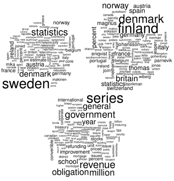
Words are known by the contexts they appear in. One can turn this contextual information to good account and infer semantic and syntactic properties of a word. Word representations are real-valued vectors that accurately capture these proper-ties. We learn a k-dimensional vector for each word such that the vectors of word pairs that behave similarly in a language tend to have a smaller Euclidean distance between them than those that don’t behave similarly. Consider, for example, the words Finland and Sweden. We see from Figure 1 that the contexts they appear in are largely similar and therefore expect these words to be either semantic or syn-tactic cognates and the vectors learnt for these words to have a small Euclidean distance. However, the contexts of any one of these words, sayFinland, differs quite drastically from those ofstocks as shown in Figure 1. The vectors learnt for Finland
andstocks therefore have a very large Euclidean distance between them. One utilises
the contexts of a word to unsupervisedly learn its vector representation. This re-sults in words that have similar contexts having similar vector representations. This simply implies that similar words have smaller Euclidean distances amongst their vector representations. This property can be, for instance, used in retrieving all the synonyms of a given word.
LetV be the total number of unique words (the size of the vocabulary) in the corpus D. The input to the Bayesian model is given as running text, where each word and its left and right contexts are hashed into an integer between 0 and |V|, succinctly representing a sparse binary vector. A hashed word w and its hashed contexts
c ∈ C(w) can thus be modelled as entries in a sparse vector of dimension 1× |V|. Such a vector xw for w is set to one for all c∈ C(w) and to zero otherwise, known traditionally know in the word embeddings literature as theone-hot representation
Figure 1: The words appearing as contexts of Finland (top left) and Sweden (top right). Since the contexts of these two words overlap to a significant extent, we could argue that the Finland and Sweden share syntactic and semantic properties. However, the contexts of either of these words differs significantly from those of
stocks (bottom). Thus, the vectors learnt for Finland and Sweden would have a
small Euclidean distance with each other. The Euclidean distance between the vectors of either Finland orSweden and stocks is much higher.
[TRB10]. Usually, all c0 6∈ C(w) implicitly are assumed to be zero. For |D| such
tokens, this constitutes a sparse binary matrix X. It is this matrix that we seek to factorise as a product of Uand V.
In typical matrix factorisation problems the dimension of U is |D| ×k and that of
in X with a corresponding unique latent entry in U. However, we recognise that not all tokens of |D| are unique and that several of them correspond to a unique word that can be represented as a single latent entry in U. To account for this, we instead use aUof dimension |V| ×k. Thus every occurrence ofw∈ Dis mapped to a unique uw ∈U. Furthermore, since the entries of Xare sparse, we propose to use the logistic model for factorisation instead of the more typical Gaussian model. This affords us the flexibility to either actively penalise everyc0
6∈C(w) or simply ignore those c0
6∈ C(w) that could potentially appear in a later token of the same word. Having defined our model, we employ variational inference to induce the actual word embeddings over the corpus. To make our model scalable, we use two variants: firstly, we employ stochastic variational inference; secondly, we use a multithreaded implementation. This results in a latent embedding uw for every w that accounts for all possible contextsw appears in.
[CWB+11] first showed how these word representations come in handy in augmenting
such tasks as chunking, semantic role labelling and named entity recognition. Since then [DRFU12], [MCCD13], [LL13] and [LC14] have improved upon these results to furnish better and better embeddings. In this thesis, the Bayesian model we present not only infers embeddings with good semantic properties but is also the first to offer continuous Gaussian densities as part of its inference process.
1.2
Contributions
This thesis presents a matrix factorisation model that attempts to model word-context tuples as lower-dimensional vectors with high predictive accuracy. Such vectors can be used to bolster existing NLP systems and push the state-of-the-art. The following contributions feature prominently in this work:
1. A crystallisation of the best practises from previous literature on word embed-dings and matrix factorisation into a single hierarchical Bayesian model. 2. We derive and implement a scalable, stochastic binary matrix factorisation
model for huge sparse binary matrices. Such a model finds use not only in inducing word embeddings, but also in movie recommendation tasks and doc-ument subspace clustering [ZLDZ07].
3. Representation of the latent dimensions as continuous Gaussian densities in-stead of as point estimates.
1.3
Layout
Chapter 2 provides a brief mathematical background. Chapter 3 on word represen-tations gives a brief review of a formal definition of vector space representation as well as a host of previous works done on it. Chapter 4 develops a Bayesian matrix factorisation model that will be used in learning word embeddings. Chapter 5 will list a few practical tweaks that we add to make the inference in the Bayesian model scalable and practical. We present our results in Chapter 6. Chapter 7 draws con-clusions and briefly retrospects our various claims, while Chapter 8 enumerates a few possibilities that could be adopted as extensions to the existing model.
2
Mathematical Background
But if you call me Anne, please call me Anne with an ‘e’
Anne of Green Gables
We saw previously how we run into difficulties in Bayesian inference during estima-tion of p(Z|D) owing to its intractability. One solution is to use an Expectation-Maximisation style algorithm, by calculating the log likelihood expectation of the data over the posterior distributions of the parameters. However we run into one of the following problems [Bis06]:
1. The dimensionality of the latent space is too high to work with, prohibiting numerical integration.
2. The complexity of the posterior distribution renders computing expectations analytically intractable with no closed-form solutions.
Variational approximation provides a deterministic framework by allowing us to approximate the posterior by
1. Allowing the distributions to have parametric forms, such as the exponential family, which in addition to being summarised by sufficient statistics have conjugate priors.
2. Allowing specific factorisations over the posterior (called mean field factorisa-tion [Par88]).
In this chapter we briefly introduce the exponential family and how it relates to the variational scheme.
2.1
Exponential Family
A member of the exponential family of distributions overx can be represented as
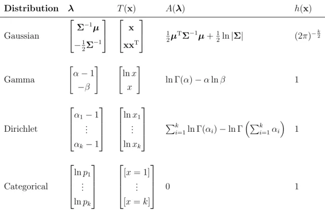
Distribution λ T(x) A(λ) h(x) Gaussian Σ−1µ −1 2Σ −1 x xxT 12µTΣ −1 µ+1 2ln|Σ| (2π) −k 2 Gamma " α−1 −β # " lnx x # ln Γ(α)−αlnβ 1 Dirichlet α1−1 .. . αk−1 lnx1 .. . lnxk Pk i=1ln Γ(αi)−ln Γ Pk i=1αi 1 Categorical lnp1 .. . lnpk [x= 1] .. . [x=k] 0 1
Table 1: Some common distributions represented as exponential family distributions. Here,
λ constitutes the natural parameter, T(x) constitutes the sufficient statistics, A(λ) constitutes the log normaliser,
h(x) constitutes the base measure.
Note that xcould be discrete or continuous, scalar or vector. In fact, most familiar distributions can be recast as a member of the exponential family. Some common examples are shown in Table 1.
2.2
Conjugate priors
The usefulness of the exponential family becomes more apparent when we realise that each of its members has a conjugate prior which can be represented as
p(λ|χ, ν) =f(χ, ν) exp(λ>χ−νA(λ))
where ν is the number of observations to which the prior contributes, χ is the number of pseudo-observations contributing to the sufficient statistics and f(χ, ν)
is a normalisation constant. νA(χ) is the log-normaliser and can also be re-written as
p(λ|χ, ν) =f(χ, ν)g(λ)νexp(λ>χ).
Consider now the data setD ={d1. . .dn} where
p(D|λ) =Y i p(di|λ) =Y i h(di)g(λ) exp(λT ·T(di)) =Y i h(di)g(λ)nexp(λT · n X i T(di)).
The posterior can thus be defined as
p(λ|D,χ, ν)∝p(D|λ)p(λ|χ, ν) =g(λ)nexp(λT · n X i T(di))·g(λ)νexp(λ>χ) +const =g(λ)ν+nexp(λ>χ+λT · n X i T(di)) +const.
Owing to conjugacy the posterior has the same functional form as the prior and is defined as p(λ|D,χ, ν) = p(λ|χ+ n X i T(di), ν+n).
The sufficient statistics alone are enough to infer the posterior of λ.
2.3
Variational Approximation
Consider the marginal likelihood p(D) of the data set D which is also intractable. That is,
p(D) = Z
p(D, θ)dθ
where θ includes the parameters as well as the latent variables and are more often than not vector-valued. The variational approximation [Att99] introduces a para-metric distribution q to approximate true posterior:
lnp(D) = ln Z q(θ)p(D, θ) q(θ) dθ ≥ Z q(θ) lnp(D, θ) q(θ) dθ =L(q).
lnp(D) L(q)
KL(qkp)
Figure 2: Variational Bayes in a nutshell [Bis06]: L(q)lower bounds the log evidence
lnp(D). To achieve the best bound, we maximise L(q) over q, which effectively minimises KL(qkp)letting q approximate pbetter.
The KL divergence between the two continuous distributions q and p is given as [Bis06]
KL(qkp) =
Z
q(θ) ln q(θ) p(θ|D)dθ
and the expected lower boundL(q) as, L(q) =−
Z
q(θ) ln q(θ) p(θ,D)dθ.
This leads to the following equivalence between the KL divergence and the marginal likelihood: KL(qkp) = Z q(θ) ln q(θ) p(θ|D)dθ = Z q(θ) ln q(θ) p(D, θ)dθ+ lnp(D) =−L(q) + lnp(D).
The relationship betweenL(q), KL(qkp) and lnp(D) is given in Figure 2. As KL is non-negative, lnp(D)≥ − Z q(θ) ln q(θ) p(D, θ)dθ = Eq[p(x, θ)]−Eq[q(θ)] =L(q).
In other words, L(q) lower bounds the marginal log likelihood. To achieve the best bound, we maximise L(q) overq, which effectively minimises the KL(qkp). Of course, we see that L(q) is intractable as well. To evaluate L(q), we will assume a factorised form ofq(θ), to wit, q(θ) =Q
iq(θi) whereθi are the parameters we need
to optimise over. We then do a gradient-based optimisation for each q(θi), ∇λlL =∇λlEq[lnp(D, θ)]− ∇λlEq[lnq(θ|λ)].
This so-called mean field factorisation allows one to factorise q(θ|λ) as, q(θ|λ) = Q
iqi(θi|λi). Let us suppose each of q(θi|λi) is a member of the exponential family.
Then, they have the following parametrisation:
qi(θi|λi) =h(θi) exp(λ>i t(θi)−A(λi))
=h(θi) exp(λ>i
∂A(λi) ∂λi −
A(λi)).
This leads to,
∇λlEq[lnq(θi|λi)] = ∂ ∂λi (λ>i ∂A(λi) ∂λi − A(λi)) =λi ∂2A(λi) ∂λi∂λ>i =λiV(λi).
Similarly for p(D, θ), if a is the Markov blanket of θi – constituting its parents, its
children and its children’s other parents – and Sa = Eq(lnpa(D, θ)), each in the
conjugate exponential family
∂Sa ∂λi
=V(λi)Eq[ηa(x, θ−i)]
where ηa(x, θ−i) constitutes the natural parameter. Thus, ∇λlL =V(λi)Eq[ηa(x, θ−i)]− V(λi)λi =V(λi)(Eq[ηa(x, θ−i)]−λi) = 0 =⇒ λi = X a Eq(ηa(x, θ−i)).
In summary, we can write the update equations tersely as follows
Algorithm 1: Mean Field Variational Bayes.
input : The data set D and appropriately parametrised q(θi|λi) ∀i∈[1, w]
output:λi, ∀i
1 while evidence lower bound L not converged do
2 for i←1 to w do
3 q(θi|λi)∝exp(Eq−i[lnp(D, θ)])
leading to the alternate maximisation scheme presented in Algorithm 1.
In this chapter we presented a deterministic framework to approximate the posterior
p(θ|D) by q(θ) factorised as q(θ) = Q
iq(θi|λi) where each q(θi) belongs to the
conjugate exponential family parametrised by λi with the posteriors retaining the
same distribution as the prior. We then resort to alternative optimisation techniques such as in Algorithm 1 to iteratively estimate the values of λi that minimise the
expected lower bound. We will in later sections introduce more efficient optimisation algorithms that scale well over large data sets.
3
Word Representations
“Words aren’t made – they grow” said Anne.
Anne of the Island
Noscitur a sociis or the notion that a word is known by the company it keeps, is
probably as old and intuitive a concept as language itself – we often catch ourselves teasing out a word’s meaning with a little hand from its neighbours. This was first formalised in linguistics by Zellig Harris2, when he stated that “The degree of semantic similarity between two linguistic expressions A and B is a function of the
similarity of the linguistic contexts in which A and B can appear”.
It comes as no surprise then that this notion can be extended to draw plausible con-clusions about the semantic nature of words. Simply put, words occurring in similar contexts are semantic cognates. Such relations have a broad and sweeping coverage in that they accommodate anything from synonyms and antonyms to hypernyms and hyponyms within their purview.
Luckily, this intuition is easily translated into simple probabilistic models that ad-equately capture the semantic properties. The resulting representations drawn are inherently valuable as they encode the predictive nature of a word as a vector. How-ever, their real worth is manifest in their power to push the current state-of-the-art systems – essentially improvements that cost nothing in terms of human labour3.
As an illustration, consider the words Harvard, Stanford and Princeton. We intuit that since these all are private universities in the United States, they are bound to have similar neighbours in a good part of their occurrences. It wouldn’t be unreasonable to expect words like graduate, school or university to occur in their vicinity. We list down for the benefit of the reader the top occurrences of each of these words. If the word representations are accurate at all, this triad should have similar representations. We will later see in Chapter 6 if our rationale is justified.
2We wryly observe that much of Harris’ work is absent from mainstream linguistics. Known to
cite only himself and his colleagues, he has had the courtesy largely returned. He perhaps owes it to the machine learning community for breathing new life into his work.
Figure 3: Contextual word clouds for 607 occurrences of Harvard, 367 occurrences
of Stanford and 270 occurrences of Princeton. The context window size is 2 to the
left and right. The data has been cleaned to remove stop words. That university
and professor figure so prominently in each cloud validates our claim of the three
words having similar contextual distributions.
3.1
Definition
Formally, a word representation is a vector space model, with each dimension hav-ing either an explicit or an inherent grammatical or semantic interpretation. The similarity of two such vectors is given, say, by the cosine distance. The simplest form of such a word vector is the one-hot representation with a vector the size of
the vocabulary with a single dimension turned on. At the risk of stating the obvi-ous, the sparsity and the high dimensionality result in poor parameter estimation. Our desideratum is therefore, a vector of reduced dimension with the discriminative power of the higher dimensional representation.
Consider a setD of word, context pairs(w, c)of size nwith wdrawn from a vocab-ulary of size d. Let C(w) be the set of all contexts for a given w. We model D as a sparse binary matrix X using the one-hot method described above. That is, for each row entry w, only c ∈ C(w) is turned on. The rest are assumed to be zero. This naturally yields a rather unwieldy matrix of dimensions n×d. However, we obtain a reduced dimensional approximation by factorising X=UV. Usually such factorisation is carried out by MAP estimates which are prone to overfitting [SM08]. Alternatively, one could probabilistically cast X as a linear model with Gaussian noise [SM08]. That is, xi ∼ N(u>
i V, τI). While [SM08] suggested a Gibbs sampler
for inference, another option is to employ variational methods elaborated in Section 2.3. The resultant lower dimensional U captures several semantic and syntactic properties of the words.
We shall now discuss different kinds of word representations in literature and their limitations.
3.2
Global Representations
Distributional representations rely on the global co-occurrence matrices of words, where each row corresponds to the co-occurrence frequencies of a word with all its contexts, to generate reduced dimensional representations. This includes the widely popular Latent Semantic Analysis (LSA). LSA [LD97] works by performing
Singu-lar Value Decomposition (SVD) on the global co-occurrence matrix X = UΣV>
where U is an orthogonal matrix of the eigenvectors of XX>, V is an orthogo-nal matrix of the eigenvectors of X>X, and Σ is diagonal matrix with the square
roots of the non-zero eigenvalues of XX> as its diagonals. Choosing the k largest
eigenvalues corresponds to ak-dimensional reduction, which is the best least square approximation to the original matrix X.
[Kas98] introduced a random-mapping based dimensionality reduction Z = RX>
where R is a random matrix with normalised columns and Z is the matrix with reduced dimensionality d. Given a0,b0
∈ Z and a,b ∈ X, we see that a0>b0 = a>R>Rb. Representing the matrix R>R as I+
[Kas98] proved that E(i,j) = 0 and σ2
≈ 1d. Clearly, the higher the value of d, the better the approximation is. More specifically, if a0>b0 = a>b +δ, where
δ = P
k6=lk,lakbl, it was proved that E(δ) = 0 and σ2δ ≤ 2σ2 ≈ 2d. That is, the
distortion of a0>b0
has zero mean and a variance of at most 2d.
[LB96]’s Hyperspace Analogue to Language (HAL) select columns with the highest variances from the co occurrence matrix X as the latent dimensions while [VH05] uses Independent Component Analysis (ICA) to transform X to a lower dimen-sion. However, distributional techniques have proved to be expensive in general, and [TRB10] claims that the exact settings necessary for a distributional represen-tation to be used for prediction tasks such as parsing and for labelling tasks such as chunking is not well understood.
3.3
Cluster-based Representations
As early as 1992, Brown et al [BdM+92] in their seminal paper attempted to build a coherent n-gram based language model that was capable of predicting a word from the previousn words and developed strategies to assign these words to classes based on the frequency of their co-occurrence with other words. Suppose f : V 7→ C is a function that maps each wordw∈V to a word classc∈C, where |C|<<|V|. One then defines a n-gram class based model as
p(wk|wk−11 ) = p(wk|ck)p(ck|ck−11 ) ∀k ∈[1, n].
Fork = 2, [BdM+92] defined the quality of such a mappingf as L(f) = 1 nln Y p(wi|ci)p(ci|ci−1) = 1 n X w,w0 lnp(w|c)p(c|c0) =X w p(w) lnp(w) +X c,c0 p(c, c0) ln p(c, c 0) p(c)p(c0) =−H(w) +I(c, c0).
where H(w) is the entropy of the unigram word distribution and I(c, c0) is the
average mutual information of the adjacent classes. [Lia05] presents an optimised clustering algorithm defined in terms ofI(c, c0). A disadvantage of [BdM+92] is that
it is limited to bigram contexts alone and has to be redefined for larger context windows. This largely cripples the scalability of the bigram model, which is perhaps its only selling point.
3.4
Distributional Representations
In contrast to earlier representations, distributed representations rely on their imme-diate contexts to generate dense, low-dimensional and real-valued representations. Collobert et al. [CWB+11] in their phenomenal paper presented a unified neural network model to demonstrate that such word embeddings could be used for regular NLP tasks such as chunking, semantic role labelling and named entity recognition. While it was impressive as a demonstration of the use of word embeddings, it per-formed abysmally in comparison to later work, both in terms of predictive accuracy and training time.4 [MH07] presented a log-bilinear algorithm that learnt a neural
network that predicted the embeddings of thenthword given the embeddings of the
previous n−1 words.
3.4.1 word2vec
If c ∈ C(w) is the context for w ∈ V, then the skip-gram model is defined by the objective function: arg max vcvw X w∈C X c∈C(w) lnp(c|w) p(c|w) = exp(v > c vw) P c∈Cexp(v>cvw) .
In order to maximise the predictive power of a word, we take the gradient oflnp(c|w). However, computing ∇lnp(c|w)is rendered impractical by the summation term in the denominator. If, instead, one replaces the softmax function with a logistic function,σ(x) = (1 +exp(x))−1 the objective becomes
arg max vcvw X w∈C X c∈C(w) σ(v>c vw)
which is trivially maximised by settingv>
wvc to arbitrarily large values.
[MCCD13] uses the skip-gram model and presents negative sampling, an idea bor-rowed from [GH12] as an efficient way to induce word embeddings. In order to discourage trivial solutions, one introduces (c, w) samples that do not exist in the corpus (hence, negative sampling) modifying the objective to
arg max vcvw X w∈C, c∈C(w) σ(v> c vw) + X w∈C, c06∈C(w) σ(−v> c0vw) .
4[LL13], as a sane afterthought to their neural network architecture, proposed using Hellinger
distance based PCA on the co-occurrence matrix of words. Since the word distributions are in-herently discrete, metrics such as the Bhattacharya and the Hellinger distance are well suited for measuring the divergence between them.
It has been shown empirically that setting the noisy distribution to 34th of the un-igram probabilities of the word works reasonably well. Recently, [GL14] proved that the embeddings induced by [MCCD13] constitute implicit matrix factorisa-tion, where the matrix to factorise consists of as its entries the point-wise mutual information between a word and its context.
3.4.2 Multi-view embeddings
[DRFU12] proposed using Canonical Correlation Analysis (CCA), a cousin of Prin-ciple Component Analysis (PCA), for pairs of matrices. For any two matrices L
andR, CCA finds a pair of linear projectionsΦL andΦR, such that the correlation
between LΦL and RΦR is maximised. This can be formally represented as
maxp E[hL,ΦLihR,ΦRi]
E[hL,ΦLi2]E[hR,ΦRi2]
.
[DRFU12] claim that whilst assuming the n-gram model for natural language, the two left and right contexts are conditionally independent given the current word, forming the two views of the CCA. They posit that by exploiting the multi-view nature of such data, the resultant dimensionality reduction retains much of its pre-dictive power. If L were to denote the left context matrix, R the right context,
C= [L R] the entire context, and Wthe word matrix, the one-step CCA is
formu-lated as
CCA(W,C) =⇒ (A,ΦC)
and two-step CCA is defined as
CCA(L,R) =⇒ (ΦR,ΦR),
S ⇐= [LΦL,RΦR],
CCA(S,W) =⇒ (ΦS,ΦW).
[DRFU12] provides further multi-view models which we shall not discuss as they are simply modified versions of CCA with randomised SVD as a preprocessing step. We contend that the efficacy of CCA is not so much because of its taking into account the multi-view nature of the data as of its proper factorisation of its con-textual matrices. In fact, in practice we have found that the left and right view are distributionally similar and there is no significant gain in viewing them as two sep-arate, independent entities. Our contention is not entirely without rationale as the Hellinger PCA[LL13] has produced evaluation scores much better and faster than
the CCA algorithm. Rather than use negative sampling, they inadvertently model the missing contexts rather than the contexts themselves. Since they do it so per-fectly and since the latent features correspond to the tokens themselves rather than the unique vocabulary items, falsely modelling missing data as negative instances does not affect their model adversely.
3.5
A Final Word
Before we begin and define our model, we make some observations and examine a few deficiencies in the extant ones:
1. We note that all previous word embedding literature uses empirical means to set the value of k, the dimension of the latent embeddings.
2. Insofar as the current methods are concerned, they all limit themselves to a given (albeit large) data. None of them are designed to work on data streams. We propose a method that can learn on practically infinite data in addition to a scalable algorithm from large but finite data.
3. The performance of word embeddings requires significant fine-tuning. Every new publication has either been a claim of pushing the state-of-the-art, or oddly enough, a retraction of a previous result. Hence we strongly suspect that these are fine-tuned to a given data set and task for optimal performance. In the following chapters, while we certainly hope to beat or match a few such benchmarks, our primary goal is to build an algorithm that is scalable and
stochastic
4. Finally, we see that none of the existing models are Bayesian. As far as we know, ours is the first practical, completely Bayesian model to induce word embeddings. It will also be the first such model to induce continuous Gaussian distributions on the latent features instead of producing point estimates. This comes at a steep price though – we will have to model the covariance matrix for each vocabulary item.
This concludes our discussion of the existing literature on word embeddings. In the next chapter we address the issue of designing a feasible Bayesian model for word embedding induction.
4
Factor Analysis of Sparse Data
Everything that’s worth having is some trouble. . .
Anne of Avonlea
We had already described, albeit briefly, how the skip-gram model introduced by [MCCD13] implicitly constitutes matrix factorisation – an observation reinforced by promising view-specific CCA results obtained by [DRFU12]. In this chapter we shall formally introduce Bayesian methods for matrix factorisation and CCA and describe an efficient and scalable Bayesian model for factorising extremely sparse binary matrices.
4.1
Matrix Factorisation
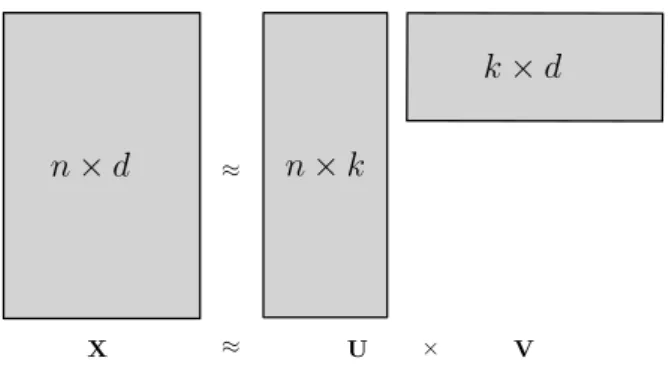
Matrix factorisation refers to the decomposition of a matrix into a product of two or more matrices as shown in Figure 4, usually with a mind to capture the interaction between two entities in terms of a lower-dimensional latent features.
n×d X n×k U k×d V ≈ ≈ ×
Figure 4: Matrix factorisation: The matrix Xn×d with n rows each of dimension d, which is presumably high dimensional is factorised into two matrices Un×k and Vk×d where k << d. In matrix factorisation literature the entries of U are known
as the latent features orfactors and those of V are known asfactor loadings.
One of the most famous applications of matrix factorisations is arguably the rec-ommender system[RV97]. For example, a large, sparse user-item matrix could be factorised into two smaller ones allowing us to determine relationships between users and between items or recommend items to users of similar interest[PKW14].
z xx x2 x1 z x2 x1 y z2 z1 x2 x1
Figure 5: Graphical models for Bayesian factor analysis (left); CCA with shared latent variables (centre); CCA with view specific latent variables (right) – this is hardly ever used in practice.
4.2
Bayesian Factor Analysis
Matrix factorisation involves modelling correlations in higher-dimensional data as a lower-dimensional, oriented subspace [Bea03]. Consider a matrix X ∈ <d×n
gen-erated by a linear transformation of a zero-mean, unit-variance Gaussian matrix
U ∈ <k×n
and some additional zero mean diagonal covariance Gaussian noise , where k≤d,
X =U>V+
Ui ∼ N(0,Ik) i ∼ N(0,Ψd)
where V ∈ <k×d
constitutes the linear transformation, also known as the factor
loadings or the projection matrix. Marginalising over Ui, it is not hard to see that
xi ∼ N(0,VV>+Ψ). By constraining the noise to be a diagonal covariance ma-trix, the xi becomes conditionally independent for a given ui [TB99]. This results in the i capturing the variation unique to an axis, while V captures the rest of
the correlations presumed to be of interest. The components of the resulting latent vectors Ui are uncorrelated. Factor analysis differs from traditional PCA in that it differentiates between the variance and the correlations. This can be rectified by replacing Ψ with an isotropic covariance, in which case the model reduces to PCA. Incidentally, for a transformation such asXi →AXi factor analysis is covariant un-der component-wise rescaling whenA is diagonal, while Bayesian PCA is covariant under rotation when A is orthogonal [TB99].
4.3
Bayesian Canonical Correlation Analysis
CCA seeks to find linear components that capture correlations between two multi-variate data sets. Given to two sets of random vectorsX1 ∈ <d1×n
and X2 ∈ <d2×n
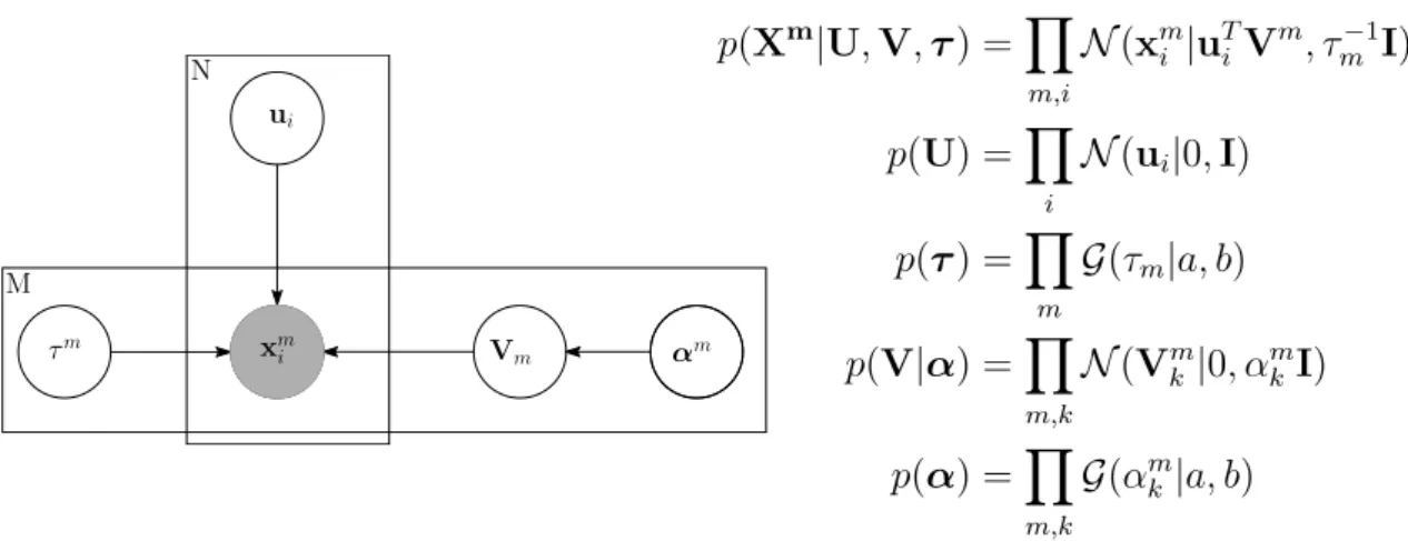
xm i Vm ui τm xm αm i N M p(Xm|U,V,τ) =Y m,i N(xmi |u T i V m , τm−1I) p(U) =Y i N(ui|0,I) p(τ) =Y m G(τm|a, b) p(V|α) =Y m,k N(Vm k|0, α m kI) p(α) =Y m,k G(αm k|a, b)
Figure 6: Plate diagram for the Bayesian CCA: Each entry in a given view xm
i is
modelled as a linear transformation of the latent vector uiVm with some added
noise. The dimensionality of Vm is automatically inferred. For CCA M = 2, while
[VKKK14] presents presents a similar model forM ≥2.
correlation between the two sets. This constitutes the first pair of new coordinates. The next pair of linear transformations maximises the correlation, conditional on it being uncorrelated to the first pair. [KVK13] presents a fully Bayesian model for CCA, shown in Figure 6.
Here, Vm constitutes the set of linear transformations for themth view. Again, the
components of vi are uncorrelated. [BJ06] presents an alternative interpretation of CCA where the latent vectors are themselves view-specific (shown in Figure 5) as well as proves Linear Discriminant Analysis(LDA) to be a special case of CCA. This model is extended to more than two views discussed at length in [VKKK14].
4.3.1 Inferring dimensionality of the latent space
Choosing k, the dimensionality of the latent space is a thorny problem. Too low a value of k would result in discarding some of the interesting correlation as noise, while too high a value of k captures spurious correlations. Automatic Relevance Determination (ARD), described in [Bis99], replaces the discrete selection ofk with a continuous prior that discourages large factor loadings. While not inferring the actual value of k, the posterior of α, when concentrated at large values effectively switches off the extraneous dimensions, resulting in only relevant factors being
al-lowed to remain active [Bis99]. ARD is modelled as p(V|α) = Y k N(Vk|0, α−1k I), p(α) = Y k G(αk|a, b).
Each hyperparameterαkcontrols the precision ofkthrow ofV, such that asαk → ∞,
the entries of thekthrow would tend to zero, resulting in the factor being ignored. As
far as we know, this little piece of ingenuity represents the first instance of automatic inference ofk5 in the word embeddings narrative.
While the extraneous rows are close enough to zero for practical purposes, sometimes we need a model that would make themexactly zero. One such alternative is use the spike-and-slab prior, where each entry in V is drawn from a two-component prior. One of these components, theslabcorresponds to the delta distribution at zero while the other, the spike is drawn from the relatively uninformative Gaussian prior. The choice between either component is provided by the Bernoulli distribution. Formally, we define the model as [KVK13]
p(Vk|Hmk, αk) = ( N(0, α−1k I) :Hk= 1 δ0 :Hk= 0 , p(Hk) = Bernoulli(π), p(π) = Beta(1,1).
whereδo is the Dirac delta function at 0. For classical CCA, the empirical approach
to inferring the latent dimensionality is to construct a scree plot of canonical cor-relations against the dimension [GDMB08]. A sharp drop between two successive values indicates that rank corresponding to the higher of the two values is the latent dimensionality [GDMB08]. Another non-Bayesian alternative is to use k-fold cross validation techniques to estimate the value of k that best explains the validation data upon reconstruction [KVK13].
4.4
Shortcomings
The Bayesian models presented hitherto pose some trouble adapting to the data we consider, namely endless tuples of words. The words – represented as one-hot
5We hypothesise that the entropy of a language plays a major role in inferring the
dimension-ality of the embeddings; one can analytically reason about how chaotic a language is from the dimensionality inferred.
vectors – result in extremely sparse binary matrices.
1. [KVK13] and most other models assume Gaussian likelihood suitable only for continuous valued data. [Kla14] refined this by introducing the Polya-Gamma augmentation [PSW13] to approximate the logistic function, also easily ex-tended to negative binomial distribution for over-dispersed count data. 2. The existing model treats each xi as a unique entry. This is simply not true
in the case of words where the entries are drawn from a vocabulary V. Thus, the latent matrix, instead of being n-dimensional should have only as many entries as the vocabulary size.
3. As we shall see in the ensuing section, approximations of the logistic function result in inversion ofk×k matrices. If we were to allocate a latent vector for each data point this would result in n inversions which is impractical to say the least. The model would not scale.
4. Finally, having latent vectors corresponding to each token requires us to come up with reasonable schemes to approximate the embedding corresponding to each unique word by considering all appearances of such a word in the data stream. This is hard owing to the transience of data streams.
Taking these above concerns into account, we detail the factorisation model of [PKW14] which replaces the Gaussian likelihood with the logistic approximation described in the next section.
4.5
Logistic Approximation
Consider the logistic functionσ(x) = 11+exp(−x). As a likelihood function, this proves
inconvenient as it destroys the conjugacy6 existent in the Gaussian likelihood. The
Jordan-Jaakkola bound [JGJS99] provides a Gaussian variational lower bound to logistic. With a little reordering,
lnσ(x) = x 2 −ln expx 2 +exp−x 2) .
6It is entirely possible to replace the conjugate updates that result from the approximation
with non-conjugate updates where the logistic likelihood is preserved. Although the asymptotic normality of the posterior ensures that posterior updates can be approximated by a multivariate normal with centred at the mode with a inverse Fisher matrix covariance, the computational cost arising as out of numerical quadratures and the complexity of the resulting derivatives serve as sufficient disincentives.
Letf(x) = ln(exp(x
2) +exp(−
x
2)). Sincef(x)is a concave function inx
2 (the second
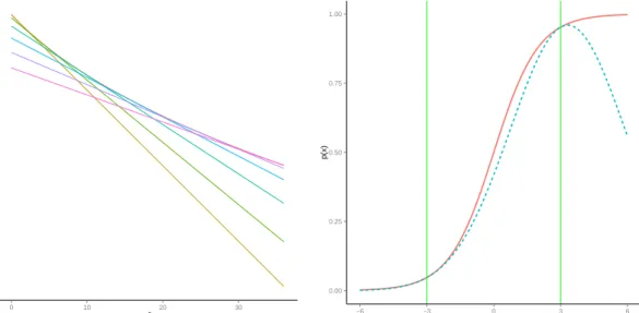
derivative being non-negative), a tangent to the f(x) – approximated by the first order Taylor expansion inx2 – is a global lower bound as shown in Figure 8. That
is, for x∈ <,
f(x)≥f(ξ) + ∂f(ξ) ∂ξ2 (x
2
−ξ2)
where ξ is the variational parameter to optimise. The bound is exact whenever
−5 −4 −3 −2 −1 0 10 20 30 (x2) p(x) 0.00 0.25 0.50 0.75 1.00 −6 −3 0 3 6 x p(x)
Figure 7: Left: f(x), a convex function in x2 is lower bounded by its first order
Taylor approximation, shown here for different values of ξ2. Right: The logistic
sigmoid function σ(x) (shown in red) is lower bounded by the Gaussian (shown in blue). The approximation is exact whenξ =±3(shown in green).
ξ2 =x2. We state that λ(ξ) = ∂f(ξ) ∂ξ2 = 1 4ξtanh( ξ 2) and, f(x)≥σ(ξ)− x 2 +λ(ξ)(x 2−ξ2).
Thus, the lower bound forσ(x)is given as
σ(x)≥exp ξ+x 2 +λ(ξ)(x 2 −ξ2) .
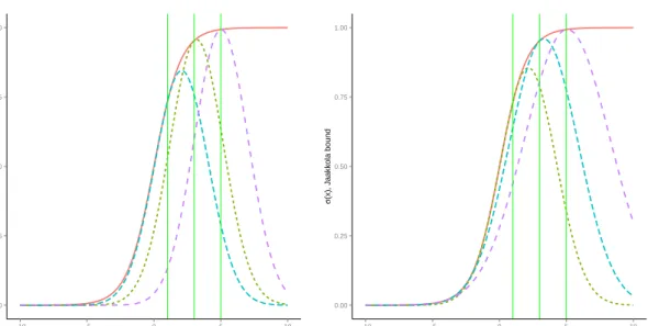
One could as well trade off some of the accuracy and tightness of the Jaakkola bound for efficiency by using the Bohning bound [Boh92], a quadratic alternative. The Bohning bound forms a second order Taylor approximation to the lnσ(x) function atξ, and replaces the Hessian H(ξ) with a constant matrix A such that A−H(ξ)
0.00 0.25 0.50 0.75 1.00 −10 −5 0 5 10 x σ (x), Bohning bound 0.00 0.25 0.50 0.75 1.00 −10 −5 0 5 10 x σ (x), J aakk ola bound
Figure 8: Left: The Bohning approximation to σ(x) at ξ = (1,3,5) the curvature of which is determined by A. The Jaakkola approximation shown at ξ =±(1,3,5)
provides a tighter bound, but is computationally expensive. We use the Jaakkola bound in our model.
bound computationally efficient, it results in fixed curvatures unlike the Jaakkola bound. For this thesis, we will stick to the tried-and-tested Jaakkola bound instead of the Bohning bound as we are unsure of the practical implications it entails.
4.6
The Case For Logistic Assumption
A word w and its contexts c ∈C(w) can be modelled as entries in a sparse vector of dimension 1× |V| where |V| is the size of the vocabulary. The vector xw for w
is set to one for all c ∈ C(w) and to zero otherwise. This is traditionally know in the word embeddings literature as theone-hot representation and has been consis-tently employed and borne out by good results [TRB10]. Arguably, this may not be the best way to represent contextual information. For instance, probabilistic data structures such as the bloom filters [MU05] could be used to concisely express the same information with reasonable accuracy. However, it is usually the case that the sparse vectors for a given w are represented as a stream(w, c) pairs for c∈ C(W)
with c6∈C(w) implicitly assumed to be zero.
The usual assumption of a Gaussian generated data with unique latent entries for each observation,xw ∼ N(u>
wV, τI)results in a bloated sparse matrix of size|D|×|V|
Gaussian assumption fails to hold when xw is a sparse binary vector. Furthermore, besides making the running time dependent on the vocabulary size |V|, this model also confuses the non-occurrence of the contextc0 6∈C(w)in an entry with its express
absence and models it as a negative instance(w, c0)
. This is not necessarily true, as a contextcnot found in a particular occurrence ofw∈ D may happen to appear in a different occurrence ofw. The drawbacks of this may not be as pronounced were we to model each observed entry xw inD with a corresponding latent entry uw. However, we recognise that tokens in D are not unique, but are instead all drawn from V. That is, each observed token w ∈ D corresponds to a unique word in V. Therefore, it seems more fitting to model all occurrences ofw∈ Das a unique latent entryuw instead of|w∈ D|distinct latent entries. In such cases, the Gaussian model performs abysmally because we begin to unnecessarily (and, indeed, quite wrongly) penalise the unique uw for non-occurrences of the contexts for a given word token. If we were to model each entry j inxi by the logistic function as,
xij = ( σ(u> i vj) :xij = 1 1−σ(u> i vj) :xij = 0
it would alleviate several problems. Firstly, this assumption is a more faithful repre-sentation7 of the data generation process. Secondly, it offers us a great deal of
flex-ibility in deciding which absences of contexts we chose to cast as negative instances and which we do not. Thirdly, it is computationally efficient and is dependent only on the window size W plus the number of negative instances as opposed to the size of the entire vocabulary V in the previous model. Finally, because the logistic assumption preempts conjugacy we use the normal approximation discussed in the previous section to replace it.
This concludes our defence of the use of the logistic link function for factorising sparse binary matrices. In the following sections we discuss at length a Bayesian model that overcomes the several barriers enumerated so far.
4.7
The Generative Story
This and the following sections draw some ideas from [PKW14]. To remain true to our assumption of truly unsupervised learning, let us assume we are presented with a corpus of natural language text, where sentences are tokenised by ([\.?!]+\s+)
and words by([[:punct:]]∗\s+). This constitutes all the preprocessing we shall do8.
Let the input arrive as tuples of the form (l, w,r), where l and r represent the left and the right contexts of the wordw. We will generically represent a single instance of the context as c. Let U,V ∈ <k×d
. We construct a hash table to map w to uw
and cto vc.
Suppose that we pickwwith probabilityπw andcwith probabilityψc. Note that we
could better model the probability of contextψcby making it conditional onw, but
we refrain from doing so. The probability of observing this tuple isσ(u>
wvc)and of
censoring it is1−σ(u>
wvc). Let us also introduce normal biasesbwandbc. Intuitively,
if w occurs in a wide variety of contexts, such as the ora, it is modelled by a large positive bias bw, while a negative bias indicates w occurs in very specific contexts.
Since we do not use it in our experiments, we shall limit ourselves to describing the idea. LetD = (T, w, c) constitute the observed set of tuples and D0 =F, the set of
unobserved, censored negative samples. We do not as yet know the value ofD0, but
according to [MCCD13] for large corpora, setting the ratio r = DD0 to 5 appeared
to work well. Let θ = (U,V,b,π,ψ) The probability of coming across a tuple
(w, c)∈ D is
p(T, w, c|θ) = πwψcσ(u>wvc+bw+bc)
while the probability of censoring an unknown tuple(w0, c0)
∈ D0 becomes a mixture overd2 components, p(F|θ) = Z p(o=F|w0, c0,θ)p(w0|π)p(c0|ψ)dw0dc0 = Z (1−σ(u>wvc+bw+bc)p(w0|π)p(c0|ψ)dw0dc0.
We model U as N(0,I), and V as a zero mean Gaussian with ARD priors. The censored data stream forms a negative background that discourages large values for
σ(u>
wvc+bw+bc). The joint likelihood of D= (D ∪ D0) is therefore given by p(D,θ) = Y (w,c)∈D σ(u>wvc+bw+bc) Y (w,c)∈D0 (1−σ(u>wvc) +bw +bc) .
We shall use Θ = ((w, c) ∈ D0,θ) to denote the entire parameter set. Having
described the intuition behind the model, we present it in the following section.
8Of course, this might be a poor idea for agglutinative language families like Finno-Ugric and
4.8
The Model
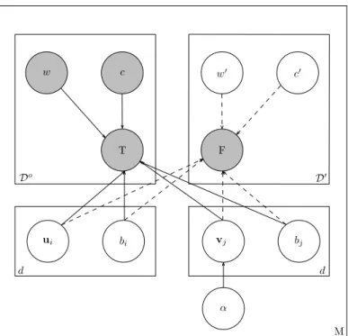
M w0 c0 w c T F ui bi vj bj α d d Do D0Figure 9: Plate diagram of the model: We draw (w, c) pairs from a uniform distri-bution. We observe D such pairs with probability σ(u>
wvc) while censoring D
0 such
pairs with probability (1−σ(u>
wvc)) assuming we know what the censored pairs
were. We employ ARD priors for dimensionality selection.
The model and its priors are shown in Figure 9. The joint probability is given by,
p(D,Θ) = Y (w,c)∈D σ(u>wvc+bw+bc) Y (w,c)∈D0 (1−σ(u>wvc+bw+bc) ×p(U)·p(V)·p(b)·p(α) where, p(U) =Y w N(uw|0,I), p(V|α) =Y m,k N(vk|0, 1 αk I), p(α) =Y m,k G(αk|a, b), p(bw) =Y w N(bw|0, τw), p(bc) =Y c N(bc|0, τc).
4.9
Variational Approximation
Let(w, c)∈ Dbe the set of observed data. The complete log likelihood of the model in Figure 9 is L(q)∝lnp(D|Θ) + lnp(Θ) = X (w,c)D Eq " lnσ(ξwc)−λ(ξwc) (u>wvc+bw+bc)2−ξ2wc +1 2(u > wvc+bw+bc)− ξwc 2 # + X (w,c)∈D0 Eq[wd0cd0]Eq " lnσ(ξwc)−λ(ξwc) (u>wvc+bw+bc)2−ξwc2 −12(u>wvc+bw+bc)− ξwc 2 # +X w Eq[lnp(uw)] + X k Eq[lnp(vk)] + X k Eq[lnp(αk)].
Approximating the intractable lnp(Θ|D) with q(Θ), we note that the lower bound to optimise becomes, lnp(D)≥ln Z pξ(D,Θ)dΘ≥ln Z q(Θ)pξ(D,Θ) q(Θ) dΘ=L(q),
where pξ(D,Θ) is joint distribution when the Gaussian lower bound replaces the logistic function so as to preserve conjugacy. We assume the following mean-field factorisation to approximate the posterior as
q(Θ) =Y w q(uw)q(bw) Y c q(vc|α)q(bc).
Finally the updates for unconstrained optimisation over each of the factor distribu-tions are
q(Θi)∝ exp Eq−i[lnp(D,Θ)]
+const or, equivalently
lnq(Θi)∝ Eq−i[lnp(D,Θ)] +const.
For the rest of this section we shall derive the variational updates for each of the parameters. For the sake of clarity, we shall state the updates as is leaving further optimisation to Section 5. Equations of relevance are starred.
4.9.1 Gaussian Updates
Consider q(U)of the form Q
wq(uw) =
Q
wN(uw|µw,Σw). The contribution ofuw
towardsL is given as lnq(uw)∝ X (w,c)∈D Eq λ(ξwc)(uw>vc+bw+bc)2 +1 2(u > wvc+bw+bc) + X (w,c)∈D0 Eq −λ(ξwc) (u>wvc+bw+bc)2 − 1 2(u > wvc+bw +bc) − 1 2tr Eq[uwu > w]I . Rearranging, lnq(uw)∝ − 1 2trEq[uwu > w] I+ X (w,c)∈D 2λ(ξwc)Eq[vcvc>] + X (w,c)∈D0 2λ(ξwc)Eq[vcvc>] +Eq[u>w] X (w,c)∈D 1 2+ 2λ(ξwc)Eq(bw+bc) − X (w,c)∈D0 1 2+ 2λ(ξwc)Eq(bw+bc) Eq[vc] .
This clearly has a the form of a Gaussian posterior and the updates for q(uw) are given by Σw = I+ X (w,c)∈D 2λ(ξwc)Eq[vcvc>] + X (w,c)∈D0 2λ(ξwc)Eq[vcvc>] −1 , (?) µw =Σw X (w,c)∈D 1 2 + 2λ(ξwc)Eq(bw +bc) − X (w,c)∈D0 1 2+ 2λ(ξwc)Eq(bw+bc) Eq[vc] . (?)
This completes the updates forq(uw). The update of the parameters for eachuw is
an embarrassingly parallel task – that is, the eachuwcan be computed independently of others with no communication – and multithreading speeds up the inference greatly.
The biases again have the Gaussian formq(bi) = Q
iN(bi, µi, τi) wherei is either w
orc. The contribution of bw toward L(q) is given as
lnq(bw)∝ X (w,c)∈D Eq λ(ξwc)(uw>vc+bw+bc)2 +1 2(u > wvc+bw +bc) + X (w,c)∈D0 Eq −λ(ξwc) (u>wvc+bw+bc)2 − 12(u>wvc+bw+bc) −1 2 Eq[b 2 w]τw =−1 2Eq[b 2 w] τb + X (w,c)∈D 2λ(ξwc) + X (w,c)∈D0 2λ(ξwc) +Eq[bw] X (w,c)∈D 1 2 + 2λ(ξwc)Eq(u > wvc+bc) − X (w,c)∈D0 1 2 + 2λ(ξwc)Eq(u > wvc+bc) .
We now see the updates for q(bw) are given by
τw = τb+ X (w,c)∈D 2λ(ξwc) + X (w,c)∈D0 2λ(ξwc) , (?) µw =τw−1 X (w,c)∈D 1 2 + 2λ(ξwc)Eq(u > wvc+bc) − X (w,c)∈D0 1 2 + 2λ(ξwc)Eq(u > wvc+bc) . (?)
Similarly, the updates for q(bc)are given by
τc = τc+ X (w,c)∈D 2λ(ξwc) + X (w,c)∈D0 2λ(ξwc) , (?) µc =τc−1 X (w,c)∈D 1 2+ 2λ(ξwc)Eq(u > wvc+bw) + X (w,c)∈D0 1 2 + 2λ(ξwc)Eq(u > wvc+bw) . (?)
4.9.2 ARD Updates
The ARD updates look very similar to those of the Gaussian updates except that the prior for vc takes the form
Eq[lnp(vc)] = −1
2tr Eq[vcvc
>]
diag(α) .
The contribution of vc towardsL is given by
lnq(vc)∝ X (w,c)∈D Eq λ(ξwc)(uw>vc+bw +bc)2 +1 2(u > wvc+bw+bc) + X (w,c)∈D0 Eq −λ(ξwc) (u>wvc+bw+bc)2 − 1 2(u > wvc+bw+bc) − 12tr Eq[vcvc>]diag(α) . Rearranging, lnq(vc)∝ − 1 2trEq[vcv > c] diag(α) + X (w,c)∈D 2λ(ξwc)Eq[uwuw>] + X (w,c)∈D0 2λ(ξwc)Eq[uwuw>] +Eq[vc>] X (w,c)∈D 1 2 + 2λ(ξwc)Eq(bw+bc) − X (w,c)∈D0 1 2 + 2λ(ξwc)Eq(bw +bc) Eq[uw] .
The updates for q(vc)are then given by
Σc = diag(α) + X (w,c)∈D 2λ(ξwc)Eq[uwuw>] + X (w,c)∈D0 2λ(ξwc)Eq[uwuw>] −1 , (?) µc =Σc X (w,c)∈D 1 2 + 2λ(ξwc)Eq(bw+bc) − X (w,c)∈D0 1 2 + 2λ(ξwc)Eq(bw+bc) Eq[uw] . (?)
This completes the updates for vc. Again, we see that the updates are
4.9.3 Gamma Updates
The contribution of αk toL(q) is given by
Lξ(q) =Eq " d 2 X k lnαk m− 1 2 X k αkvk>vk+X k ((a−1) lnαk−bαk) # =Eq " d 2 + (a−1) X k lnαk− 1 2vk > vk+b X k αk # .
The updates are of q(α) are
a0 =a+ d 2, (?) b0 =b+ 1 2 X k Eq vk>vk . (?)
The value for P
kEq vk>vk is given byP ktr Eq vkvk> . 4.9.4 Logistic Bounds
[PKW14] treats the logistic bound separately for the observed values (i, j) while tying down the bound for censored observations toξ∗. Consider a given viewm. By
differentiating its contribution to L(q) w.r.t ξij, the optimal bound becomes
Lξ(q) =Eq lnσ(ξij)−λ(ξij) (ui>vj +bi+bj)2−ξij2 +1 2(u > i vj+bi +bj)− ξij 2 .
Differentiating w.r.t ξij and maximising, ∂Lξ(q) ∂ξwc =λ0(ξwc) ∂ ∂λ(ξwc)Eq lnσ(ξwc)−λ(ξwc) (u>wvc+bw+bc)2−ξwc2 + 1 2(u > wvc+bw+bc)− ξwc 2 = 0 =⇒ 0 =λ0(ξwc)(Eq[(u>wvc+bw+bc)2]−ξwc2 ) =⇒ ξ2 wc =Eq[(u > wvc+bw+bc)2]. (?)
Storing the logistic parameter for each unique(w, c)is prohibitively costly. Instead, we calculate it on the fly.
4.9.5 Biases
From the above equations it is not hard to see that dispensing with the biases leads to a reduction in the number of calculations required for an update. For example,
in the logistic updates, when the biases are done away with, the equation for ξwc
simply reduces to
ξwc=tr(Eq[uwu>w]Eq[vcvc]).
We contend that since the biases possess just informative value by giving an estimate of the contextual nature of the word, they do not prove strictly necessary for our model, losing them does not affect the quality of the word embeddings. Thus, in our actual algorithms presented in Chapter 5 we simply choose to ignore them.
4.10
Negative Sampling
The idea of negative sampling [MCCD13] is to generate a so-called negative data stream(w, c)∈ D0 that helps push the value σ(u>
wvc) down [GL14]. In the absence
of a negative stream, the likelihood for the observed data,
arg max
vcvw
X
w∈C, c∈C(w)
σ(v>c vw)
is maximised by trivially setting uw =vc such that u>
wvc=k for a large enough k.
This results in all the vectors looking the same. [GH12] first showed that by intro-ducing artificially generated noise distinct from the observed data leads to consistent estimation of parameters in logistic regression. [MCCD13] borrowed this paradigm and showed that by pushing the vectors away from certain artificially generated combinations, one obtains non-trivial solutions. Thus the modified likelihood is
arg max vcvw X w∈C, c∈C(w) σ(v>c vw) + X w∈C, c06∈C(w) σ(−v>c0vw) where c0
6∈ C(w) is appropriately sampled from suitable distribution. This is the basic intuition behind negative sampling. Note that by fixing either vc or vw, this model simply reduces to logistic regression.
We can employ a number of schemes for negative sampling the simplest being sam-pling from the vocabulary uniformly. While more complex schemes such as popular-ity based sampling as is common in recommendation system can be used, we found the uniform sampler to work just fine.
5
Scalable Bayesian Word Embeddings
As a rule, I am very careful to be shallow and conventional where depth and originality are wasted.
Lucy Maud Montgomery
Variational inference through alternating updates offers a quick and satisfactory solution although it does have a tendency to get stuck in local minima. That said, variational inference fails to scale up to large data sets – sweeping through the entire data set for each update of the parameters becomes infeasible in the long run. Recently [HBWP13] introduced a stochastic variant of variational inference, a scalable method which borrows techniques from stochastic optimisation [RM51] to optimise the objective function by obtaining noisy estimates of the gradient This overcomes the previously mentioned hurdle and helps handle massive data sets. In this chapter we offer two solutions to make our algorithm a practical one.
• In keeping with our promise of a stochastic and scalable algorithm we offer a purely SVI-type algorithm to scale up to any length of data.
• The second solution is a hybrid of batch and stochastic versions that uses a potpourri of multithreading, mini-batches and noisy downsampling to estimate a better approximation of the likelihood than one estimated by a purely SVI-based algorithm.
Before defining our algorithms, we briefly review some preliminaries for stochastic inference.
5.1
Natural Gradients
In this section we briefly review the usefulness of natural gradients for quick con-vergence. According to [HTRK08], in stochastic variational updates, the parameter space is not Euclidean. Thus the traditional gradient, that points in the direction of steepest gradient in the Euclidean case with an orthonormal coordinate system, is not accurate when the parameter space is a curved manifold with no orthonor-mal coordinates. This curved manifold is known as the Riemannian space. Let us suppose we aim at optimising an objective function with respect to a parametrised
probability distribution q(β|λ). In case of a Euclidean space, the gradient ∇λf(λ)
points in the same direction as
arg maxf(λ+dλ) kdλk2 < 2.
[HBWP13] suggests the use of summarised KL divergence as the natural measure of dissimilarity between two distributions
DKLsym(λ, λ0) =Eλ log q(β|λ) q(β|λ0) +Eλ logq(β|λ 0) q(β|λ) .
Now let us replace the Euclidean metric with DsymKL, a Riemannien metric. Then, the direction of the steepest ascent becomes
arg maxf(λ+dλ) DKLsym(λ, λ+dλ)< .
Unlike the Euclidean gradient, the natural gradient according to [Ama98] points in the direction of steepest descent in the Riemannian space and the distance between the two distributions parametrised byλand λ+dλis the change in DKLsym. For most of the probability distributions, this warping of the Euclidean manifold is done by multiplying the normal gradient with the inverse of the Fisher information matrix V where
V(λ) = E[∇λlnq(θ|λ)(∇λlnq(θ|λ))>].
In the exponential family of distributions, the Fisher information is found by taking the second the second derivative of the log normaliser A, ∂∂λi∂λ2A(λi)>
i
Recalling from Section 2.3 the natural gradient for L(q) is given by
˜
∇λlL =V(λi)−1∇λlL
where V(λi)−1 is the inverse of the Fisher information matrix. It is not hard to see
that ˜ ∇λlL =V(λi)−1∇λlL =V(λi)−1(V(λi)Eq(ηa(x, θ−i))−λiV(λi)) =Eq[ηa(x, θ−i)]−λi = 0 =⇒ λi = X a Eq(ηa(x, θ−i))
Moreover, if any factor in Sa is not in the conjugate exponential family, then ˜ ∇λlL =V(λi) −1 ∇λlL =V(λi)−1(∇λlEq[lnp(D, θ)]− V(λi)λi) =V(λi)−1∇λlEq[lnp(D, θ)]−λi) = 0 =⇒ λi =V(λi)−1∇λlEq[lnp(D, θ)].
We shall however restrict ourselves to the conjugate exponential family of distribu-tions with the neat update
λi = X
a
Eq(ηa(x, θ−i)).
5.2
Scaling up
Stochastic ascent optimises the objective function by obtaining noisy estimates of the gradient. Robbins-Munro[RM51] showed that if the step sizest at the tth iteration
satisfy the conditions
X t t=∞, X t 2 t <∞
thenλtwill converge to either the global or local optimum with the following
stochas-tic update
λt+1 =λt+
t∇˜λL.
In other words if∇˜λlLis a noisy estimate of the gradient andλˆi =PaEq(ηa(x, θ−i))
is the noisy natural parameter obtained, then
λt+1= (1
−t)λt+
tˆλi.
While theoretically a single data point can be used to obtain a noisy estimate of the gradient by multiplying the gradient estimate of that single point by the total number of data points, in practice we tend to use gradient estimates from small batches of data times the number of batches to obtain a less noisy estimate of the gradient. This leads to a simple algorithm shown in Algorithm 2.
In most cases, the variational parameters can be conveniently split into local vari-ables corresponding to each observation and global varivari-ables. Since any given local
![Figure 2: Variational Bayes in a nutshell [Bis06]: L(q) lower bounds the log evidence ln p( D)](https://thumb-us.123doks.com/thumbv2/123dok_us/9025342.2800398/15.892.369.564.104.300/figure-variational-bayes-nutshell-bis-lower-bounds-evidence.webp)