Mixture of Latent Variable Models for
Remotely Sensed Image Processing
by
Linlin Xu
A thesis
presented to the University of Waterloo in fulfillment of the
thesis requirement for the degree of Doctor of Philosophy
in Geography
Waterloo, Ontario, Canada, 2014
Author's Declaration
I hereby declare that I am the sole author of this thesis. This is a true copy of the thesis, including any required final revisions, as accepted by my examiners.
Preface Statement
The doctoral dissertation is compiled under the manuscript option, following the guidelines provided by the joint Waterloo-Laurier Graduate Program in Geography. Three manuscripts published in refereed journals, as listed below, are presented in Chapters 3 to 5 respectively, where the manuscripts are minorly changed for consistence formatting.
[1] Xu Linlin, *Li J., 2014. Bayesian classification of hyperspectral imagery based on probabilistic sparse representation and Markov random field, IEEE Geoscience and Remote Sensing Letters, 11(4): 823-827.
[2] Xu Linlin, *Li J., Wong A., Peng J., 2014. K-P-Means: A clustering algorithm of K ―purified‖ means for spectral endmember estimation, IEEE Geoscience and Remote Sensing Letters, 11(10): 1787-1791.
[3] Xu Linlin, *Li J.,Shu Y., Peng J., 2014. SAR image denoising via clustering-based principal component analysis, IEEE Transactions on Geoscience and Remote Sensing, doi.10.1109/TGRS.2014.2304298.
In all three manuscripts, I am the first author and my supervisor Prof. Dr. Jonathan Li is corresponding author. They are dominated by my intellectual effort. The roles of coauthors are explained in detail below.
The ideas in the first manuscript [1] were conceived by me. And I carried out the work, including experiments design and implementation, manuscript writing and revision. Dr. Li actively participated in the discussion of the experiment results and reviewing of the manuscript. In [2], I conceived the key ideas, conducted the experiments, wrote the manuscript and performed the revisions. The other coauthors participated in the reviewing of the manuscript. Dr. Wong provided critical suggestions on experimental design and reference choice. In [3], I initiated the research on PCA-based SAR image denoising, derived the equations in the method, designed and conducted the experiments, wrote and revised the manuscript. The other coauthors actively participated in discussion of the results and reviewing of the manuscript.
Signatures of coauthors indicate they are in agreement with the statement above.
Alexander Wong_________________________ Jonathan Li_______________________ Junhuan Peng____________________________ Yuanming Shu____________________
Abstract
The processing of remotely sensed data is innately an inverse problem where properties of spatial processes are inferred from the observations based on a generative model. Meaningful data inversion relies on well-defined generative models that capture key factors in the relationship between the underlying physical process and the measurements.
Unfortunately, as two mainstream data processing techniques, both mixture models and latent variables models (LVM) are inadequate in describing the complex relationship between the spatial process and the remote sensing data. Consequently, mixture models, such as K-Means, Gaussian Mixture Model (GMM), Linear Discriminant Analysis (LDA) and Quadratic Discriminant Analysis (QDA), characterize a class by statistics in the original space, ignoring the fact that a class can be better represented by discriminative signals in the hidden/latent feature space, while LVMs, such as Principal Component Analysis (PCA), Independent Component Analysis (ICA) and Sparse Representation (SR), seek representational signals in the whole image scene that involves multiple spatial processes, neglecting the fact that signal discovery for individual processes is more efficient.
Although the combined use of mixture model and LVMs is required for remote sensing data analysis, there is still a lack of systematic exploration on this important topic in remote sensing literature. Driven by the above considerations, this thesis therefore introduces a mixture of LVM (MLVM) framework for combining the mixture models and LVMs, under which three models are developed in order to address different aspects of remote sensing data processing: (1) a mixture of probabilistic SR (MPSR) is proposed for supervised classification of hyperspectral remote sensing imagery, considering that SR is an emerging and powerful technique for feature extraction and data representation; (2) a mixture model of K ―Purified‖ means (K-P-Means) is proposed for addressing the spectral endmember estimation, which is a fundamental issue in remote sensing data analysis; (3) and a clustering-based PCA model is introduced for SAR image denoising. Under a unified optimization scheme, all models are solved via Expectation and Maximization (EM) algorithm, by iteratively estimating the two groups of parameters, i.e., the labels of pixels and the latent variables. Experiments on simulated data and real remote sensing data demonstrate the advantages of the proposed models in the respective applications.
Acknowledgements
First, I would like to express my heartfelt thanks to my advisor Professor Dr. Jonathan Li for his guidance, support and the freedom he gave me to pursue the research areas I was interested in. Without his insight, encouragement and invaluable support, I would not have been able to complete this research.
I am also very grateful to my thesis committee members, Professors, Dr. Alexander Wong, Dr. Alexander Brenning at University of Waterloo and Dr. Michael A. Chapman at Ryerson University for their enlightening ideas and discussions, as well as critical comments and suggestions on my thesis. I also want to thank Professor Dr. Chris Lakhan, at Department of Earth and Environmental Sciences, University of Windsor for his critical and helpful comments on the thesis, and Dr. Zhiqiang Ou, Mr. Matt Arkett, Mr. Thomas Stubbs and Ms. Angela Cheng at Canadian Ice Service, Environment Canada for providing RADARSAT-1 and 2 images to support my research.
I would like to thank the financial support from the China Scholarship Council, University of Waterloo and the Natural Science and Engineering Research Council of Canada (NSERC).
Thanks also go to my colleagues at the University of Waterloo, Dr. Haiyan Guan, Yuanming Shu, Dr. Haowen Yan, Weifang Yang, Si Xie, Xiaoyong Xu, Zhenzhong Si, Xiao Xu and Peng Peng for their encouragement and friendship, and staff members in the Department of Geography and Environmental Management, University of Waterloo, Ms. Susie Castela, Ms. Lori McConnell and Ms. Diane Ridler, for helping me in various ways.
Finally and most importantly, I am deeply indebted to my parents and my wife, for their love, patience, understanding, and support.
Table of Contents
Author's Declaration ...ii
Preface Statement ... iii
Abstract ... iv
Acknowledgements ... v
Table of Contents ... vi
List of Figures ... ix
List of Tables ... xi
List of Symbols ... xii
List of Abbreviations ...xiii
Chapter 1 Introduction ... 1
1.1 Background ... 1
1.2 Motivation and Objectives ... 2
1.3 Thesis Structure ... 4
Chapter 2 Mixture of Latent Variable Models ... 6
2.1 Mixture Model ... 6
2.2 Latent Variable Model (LVM) ... 7
2.3 Mixture of LVMS (MLVM) ... 9
2.3.1 Model Formulation ... 9
2.3.2 Optimization scheme ... 10
2.3.3 Model Specifications and Variations ... 11
2.4 Models Developed under MLVM Framework ... 14
2.4.1 Mixture of Probabilistic Sparse Representation (Abbreviation MPSR) ... 14
2.4.2 K-P-Means Model ... 15
2.4.3 Clustering-based Principal Component Analysis... 17
2.5 Chapter Summary ... 18
Chapter 3 MPSR for Bayesian Classification of Hyperspectral Imagery ... 19
3.1 Introduction ... 19
3.2 Proposed Approach ... 20
3.2.1 Problem Formulation... 20
3.2.2 Mixture of Probabilistic Sparse Representation ... 21
3.2.4 Complete Algorithm ... 23 3.3 Experiments ... 24 3.3.1 Design of Experiments ... 24 3.3.2 Numerical Comparison ... 25 3.3.3 Visual Comparison ... 27 3.3.4 Sensitivity of Parameters ... 27 3.4 Conclusion ... 28
Chapter 4 K-P-Means for Spectral Endmember Estimation ... 29
4.1 Introduction ... 29
4.2 K-P-Means ... 30
4.2.1 Problem Formulation and Motivations ... 30
4.2.2 K-P-Means Model... 31 4.2.3 Abundance Estimation ... 32 4.2.4 Endmember Estimation ... 32 4.2.5 Complete Algorithm ... 33 4.3 Experiments ... 34 4.3.1 Simulated Study ... 34
4.3.2 Test on Real Hypersectral Images ... 37
4.4 Conclusion ... 39
Chapter 5 Clustering-based PCA for SAR Image Denoising ... 40
5.1 Introduction ... 40
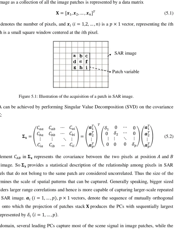
5.2 Data Formation & PCA Analysis ... 43
5.3 SAR Image Denoising in PCA Domain ... 44
5.4 Clustering Scheme ... 46
5.4.1 Feature Extraction ... 47
5.4.2 The Compatibility of PCA Features and K-means algorithm... 48
5.4.3 Parameters tuning and efficient realization ... 49
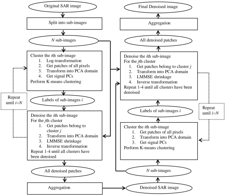
5.5 Complete Procedure of the Proposed Approach... 51
5.6 Results and Discussion ... 53
5.6.1 Test with Simulated Images ... 54
5.6.2 Test with real SAR images ... 59
Chapter 6 Conclusions and Recommendations ... 63
6.1 Summary and Contribution ... 63
6.2 Recommendations for Future Research ... 65
6.2.1 Incorporating Label Prior ... 65
6.2.2 Estimating Hyperparameters ... 66
6.2.3 Unsupervised MPSR for Clustering and Latent Variable Learning ... 66
6.2.4 K-P-means for clustering ... 66
6.2.5 K-P-Means for non-negative matrix factorization ... 67
References... 68
Appendix A List of Publications during PhD Thesis Work ... 78
List of Figures
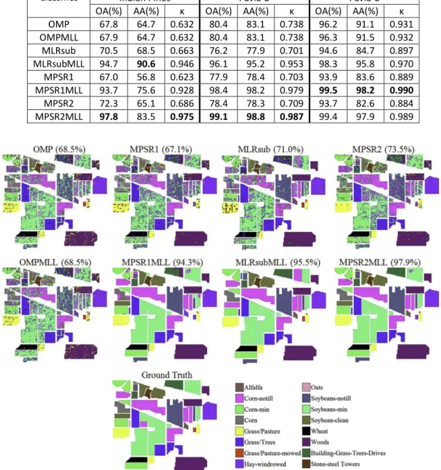
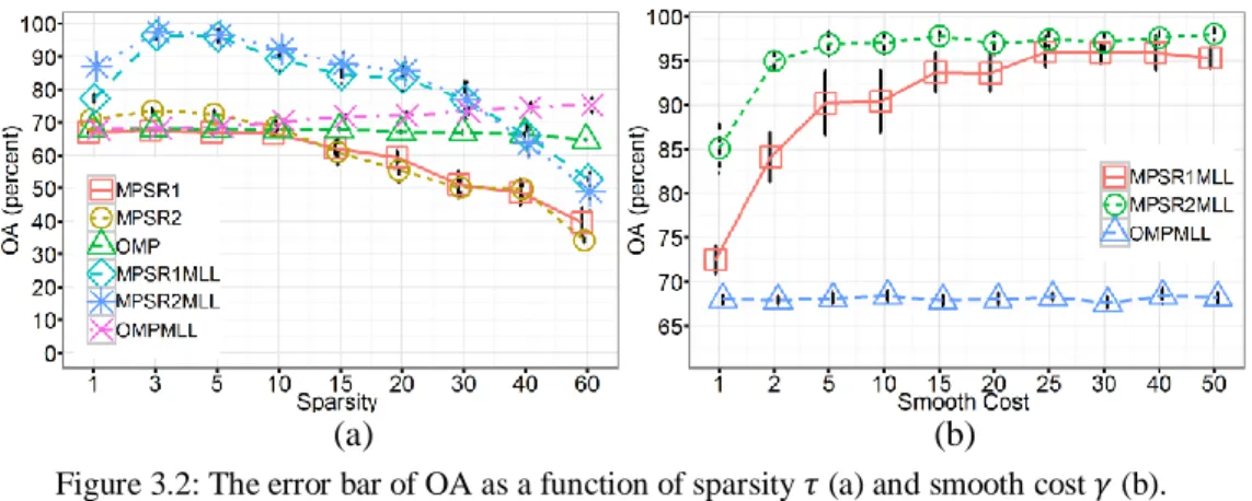
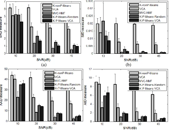
Figure 3.1: Classification maps obtained by different methods on AVIRIS Indian Pines dataset (overall accuracy are reported in the parentheses). ... 27 Figure 3.2: The error bar of OA as a function of sparsity (a) and smooth cost (b)... 28 Figure 4.1: Performance comparison at different noise levels in terms of (a) SAD, (b) SID, (c)
AAD and (b) AID. In these four statistics, smaller value means better result. ... 35 Figure 4.2: The ground-truth map of 16 classes in AVIRIS Indian Pines image. ... 37 Figure 4.3: The abundance maps of eight selected endmembers extracted by
K-P-Means-Random. ... 38 Figure 4.4: The abundance maps of the corresponding eight endmembers extracted by
MVC-NMF. ... 38 Figure 5.1: Illustration of the acquisition of a patch in SAR image. ... 43 Figure 5.2: The flowchart of the proposed algorithm (left part: stage 1, right part: stage 2). ... 52 Figure 5.3: Clean images used in this study, (a) Barbara, (b) Optical satellite image (IKONOS),
(c) Synthesized texture image. All images are 256×256 pixels big. ... 57 Figure 5.4: Zoom of Barbara image degraded by single look speckle noise, (a) clean image, (b)
noisy image, (c) PPB, (d) LPG-PCA, (e)SAR- BM3D, (f) the proposed method. ... 58 Figure 5.5: Zoom of IKONOS image degraded by single look speckle noise, (a) clean image, (b) noisy image, (c) PPB, (d) LPG-PCA, (e) SAR-BM3D, (f) the proposed method. ... 58 Figure 5.6: Zoom of synthesized texture image degraded by single look speckle noise, (a) clean
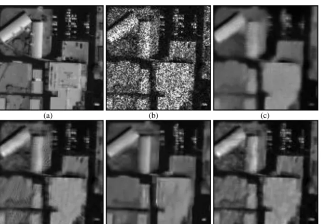
image, (b) noisy image, (c) PPB, (d) LPG-PCA, (e) SAR-BM3D, (f) the proposed method. ... 59 Figure 5.7: Zoom of TerraSAR-X SSC image (112 95 pixels) of the parking lot located at the
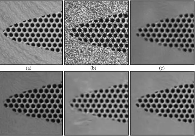
NE of the Macdonald-Cartier Freeway/Allen Road interchange, Toronto, Canada, with L=1, (a) SRAD, (b) original image, (c) PPB, (d) LPG-PCA, (e) SAR-BM3D, (f) the proposed method. ... 60 Figure 5.8: Zoom of TerraSAR-X SSC image (126 116 pixels) of the roads located at the SE of
the Macdonald-Cartier Freeway/Allen Road interchange, Toronto, Canada, with L=1, (a) SRAD, (b) original image, (c) PPB, (d) LPG-PCA, (e) SAR-BM3D, (f) the proposed method. ... 61
Figure 5.9: Zoom of TerraSAR-X MGD SE image (104 101 pixels) of the area located at 1077 Wilson Ave, Toronto, Canada, with L=2.1, (a) SRAD, (b) original image, (c) PPB, (d) LPG-PCA, (e) SAR-BM3D, (f) the proposed method. ... 62
List of Tables
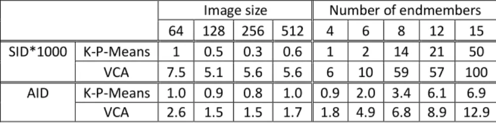
Table 3.1: Overall accuracy, average accuracy, and κ statistic obtained by different methods ... 26 Table 4.1: Performance of K-P-Means-VCA and VCA, measured by mean SID and AID, over
different image size and varying number of endmembers. ... 36 Table 5.1: Results (s/mse and ) on three images with different noise levels ... 57
List of Symbols
dimensional observation at site in class k
dimensional linear transformation matrix in class k dimensional latent variable at site in class k
dimensional noise variable in class k the th column vector in
covariance matrix of
dimensional mean vector of class k label of observation at site
unit matrix number of classes number of observations
List of Abbreviations
EM Expectation and Maximization algorithm GMM Gaussian Mixture Model
ICA Independent Component Analysis K-P-Means K Purified Means clustering algorithm LDA Linear Discriminant Analysis
LMMSE Linear Minimum Mean-Square Error estimation LVM Latent Variable Model
MAP Maximum a Posterior estimation MLE Maximum Likelihood Estimation MLL Multi-level Logistic prior
MLVM Mixture of Latent Variable Model
MPPCA Mixture of Probabilistic Principal Component Analyzer MPSR Mixture of Probabilistic Sparse Representation
MRF Markov Random Field PCA Principal Component Analysis QDA Quadratic Discriminant Analysis SAR Synthetic Aperture Radar SR Sparse Representation
1
Chapter 1
Introduction
1.1 Background
Remote sensing is the science of acquiring information about earth surface from a distance, using sensors typically onboard aircrafts or satellites (Lillesand et al., 2008). Remote sensors can be either active or passive. Synthetic aperture radar (SAR), as a typical active sensor, is capable of illuminating earth surface by microwave and collecting the backscattered waves from earth surface (Oliver and Quegan, 1998; Mott, 2007; Wang, 2008). Due to its ability to work irrespective of weather conditions or sun-light illumination, SAR has been widely used in remote sensing applications. Passive sensors, such as multispectral or hyperspectral sensors, on the other hand, capture the natural electromagnetic radiation that is reflected or emitted by earth surface. Since they obtain full spectral information with narrow spectral bands, hyperspectral sensors are good at discriminating different materials, and have been used in various applications including mineralogy, defense and environmental measurements (Richards and Jia, 1999; Shaw and Manolakis, 2002; Liang, 2004; Ustin, 2004; Lillesand et al., 2008; Bioucas-Dias et al., 2013).
While the advancement in remote sensing platforms provides great opportunities for a broad range of disciplines, the large and ever-increasing data volume demands efficient data processing and analysis techniques. The remote sensing data are usually provided as digital raster images. Therefore, image processing techniques are required to address many different tasks, such as image denoising, classification and spectral unmixing (Camps-Valls et al., 2011).
Image denoising aims to remove the undesirable information that contaminates the image. Noise in remote sensing images could be caused by many factors, depending on how the image was created. In particular, SAR sensor, as a coherent system, inherently produces speckle noise, which has salt-and-pepper appearance, and greatly impedes SAR image interpretation (Xie, et al., 2002). Noise reduction therefore always serves as a preprocessing step to enhance image quality (Buades et al., 2005).
Remote sensing image classification intends to infer the label/identity information of image pixels based on the spectral or spatial measurements (Lu and Weng, 2007; Mountrakis et al., 2011; Mulder, et al., 2011; Bioucas-Dias et al., 2013; Camps-Valls et al., 2014). Both supervised and unsupervised
techniques can achieve this purpose. Before performing classification, supervised classifiers are firstly trained on training samples with known labels, in order to learn the relationship between observations and labels. Unsupervised classifiers, on the other hand, do not need to be trained, and cluster the observations based on their internal structures.
Spectral unmixing task aims to estimate for each pixel the fractional abundances of endmembers, which are the spectra of pure materials (Plaza et al., 2009; Camps-Valls et al., 2011; Bioucas et al., 2012; Bioucas-Dias et al., 2013). The endmembers are assumed to be the underlying factors, which are responsible for generating the spectral pixels in multispectral or hyperspectral images. The estimation of endmembers as well as their abundances is a fundamental issue for remote sensing image analysis.
Remote sensing image processing is essentially an inverse problem, in which the observations are used to infer the properties of underlying geospatial processes that contribute to data generation (Wang, 2010). Therefore, knowing the data generating mechanism is crucial for solving inverse problems. If the function describing the relationship between the measurements and the underlying quantities is provided, data inversion can be solved by inverting the function. Unfortunately, in remote sensing, a function of explicit and exact form is usually unknown.
In order to achieve meaningful data inversion, prior information concerning data generation has to be used as guidance and regulation. In practice, statistical generative models are usually employed to describe the relationship between underlying quantities and measured ones, considering that stochastic generative models allow explicitly modeling the hidden variables associated with underlying generative mechanism, while in the meantime accommodating the noise in observations and uncertainties in human knowledge.
Efficient remote sensing data processing therefore relies on well-defined generative models that capture key factors in the relationship between the underlying physical process and the observations.
1.2 Motivation and Objectives
In remote sensing, three factors concerning the relationship between the observations and underlying spatial processes are of fundamental importance.
(1) Multiple spatial processes, instead of single one, contribute to generation the remote sensing images, given the complexity of the ground target. Consequently, observed image pixels of different sources tend to assume different spectral or spatial patterns. For example, an urban image usually
involves multiple ground cover types, which admit different textural structures in spatial domain, and varying spectral patterns in spectral space. Such source heterogeneity phenomenon is also witnessed at sub-pixel level. For example, an image pixel always involves the spectral contributions of multiple materials, whose spectra are called endmembers.
(2) Informative signals lie in latent space, instead of the original spectral/spatial space, due to noise and other uncertainties in remote sensing system. The unobserved variables in latent space, also called latent variables, may provide informative representation of the remote sensing data. For example, textual patterns of ground targets, as linear or nonlinear arrangements of pixels values, may serve as signatures of different land cover types. In addition, the latent variables may offer explanations of the data generation mechanism. For example, the abundances of endmembers reveal the material composition of a mixed pixel. Moreover, the latent variables can also help to reduce the dimensionality of high-dimensional measurements, which are not rare in remote sensing.
(3) Different spatial processes tend to associate with different groups of latent variables, instead of by the same group. For example, different ground cover types tend to admit different spectral signatures in latent spectral domain, and assume varying types of texture patterns in latent spatial space.
Due to the co-occurrence of above three factors, efficient data analysis therefore relies on well-defined generative models that are capable of accounting for both source heterogeneity effect and hidden variable effect, as well as their relations. Unfortunately, as two mainstream data analysis techniques, mixture models and latent variables models (LVM) are inadequate in addressing these important issues.
On the one hand, mixture models, such as K-Means, Gaussian Mixture Model (GMM), Linear Discriminant Analysis (LDA) and Quadratic Discriminant Analysis (QDA), although being capable of accounting for the effects caused by different sources, fail to address the latent variable effects. Consequently, the learning of mixture components will be rendered inefficient, due to the failure in addressing their association with latent variables. For example, since GMM characterizes a class by Gaussian distribution in the original space, and ignores the fact that classes could be better represented by discriminative signals in the hidden/latent feature space, it is difficult for GMM models to strike a good balance between model bias and model variance.
On the other hand, LVMs, such as Principal Component Analysis (PCA), Independent Component Analysis (ICA) and Sparse Representation (SR), explain only the latent variable effects, but fail to account for the source heterogeneity issue. As a result, the learning of latent variables will be affected and disturbed by the existence of mixture effect, due to the failure to explicitly model such effect. For example, because PCA seeks representational signals in the whole image scene that involves a mixture of sources, and neglects the fact that signal discovery for individual sources is more efficient, in image denoising problems, global PCA learnt for all classes is less efficient than local PCAs learnt for individual classes. In order to avoid confusion, it is worthwhile to mention that LVM here refers to continuous latent variable models.
Driven by the above considerations, this thesis therefore intends to explore mixture of LVM (MLVM) that is capable of accounting for both mixture effects and latent variables, in order to achieve efficient remote sensing data processing techniques. Although some MLVM models, such as mixture of probabilistic PCA (MPPCA, Tipping and Bishop, 1999) and mixture of factor analyzer (MFA, Ghahramani and Hinton, 1996; Fokoue and Titterington, 2003) have been developed in the statistical literature, no efforts have been conducted towards a systematic investigation, in the context of remote sensing data processing. Four main research questions or gaps remain unaddressed, which motivate the studies conducted in this thesis.
(1) There is still a lack of a general framework that is capable of providing principles and guidelines for building MLVMs that suit a variety of remote sensing data processing tasks.
(2) MLVM has not been developed for SR, which is emerging and powerful technique for feature extraction and data representation.
(3) Since the pixel values in remote sensing images are nonnegative, the latent variables are also required to be nonnegative in some cases, e.g. spectral unmixing. Therefore, new MLVMs have to be developed to address this particularity of remote sensing data.
(4) The diversity of remote sensing data type and applications requires new MLVMs that support different remote sensing data processing tasks, e.g. denoising, classification, spectral unmixing.
1.3 Thesis Structure
This thesis proposes to study the modeling and analysis of remotely sensed imagery from a probabilistic generative perspective. Simultaneous modeling of both the underlying spatial processes and hidden signals is achieved by MLVMs, where mixture components distinguish between different
spatial processes, and latent dimensions account for hidden signals in each component. The contribution of this thesis lies in the following aspects:
Chapter 2 introduces a probabilistic framework, enabling a principled way of modeling and estimating both source heterogeneity effect and hidden signal effect, under which three MLVMs are developed, and successfully applied to a variety of remote sensing applications in terms of the image processing tasks and the sensor types.
Chapter 3 describes a novel mixture of probabilistic SR (MPSR) model, to be incorporated with Markov random field (MRF) for supervised classification of hyperspectral remote sensing imagery, considering that SR is an emerging and powerful technique for feature extraction and data representation.
Chapter 4 presents a novel mixture of K Purified means (K-P-Means) model, for spectral endmember estimation, which is a fundamental issue in remote sensing data processing.
Chapter 5 presents a clustering-based PCA algorithm in Chapter 5, for state-of-the-art SAR image denoising.
Chapter 2
Mixture of Latent Variable Models
This Chapter starts with an overview of the mixture model and LVM, followed by the introduction to the framework of MLVM, and the descriptions of three variants of MLVM.
2.1 Mixture Model
Since multiple spatial processes are responsible for remote sensing data generation, mixture models, which account for this source heterogeneity effect, are essential for pattern discovery and prediction (McLachlan and Peel, 2000). In mixture models, the dimensional observation at site in class k, denoted by , can be expressed as a linear combination of the mean vector of a class , plus the class-dependent noise :
(2.1) Mixture models differ on noise distributions (McLachlan and Peel, 2000). In particular, the GMMs are widely used for the tasks of clustering and classification of remote sensing data (e.g. Ju et al., 2003; Clark et al., 2005; Amato et al., 2008; Thessler et al., 2008; Brenning, 2009; Pu and Landry, 2012; Chen et al., 2013), where is Gaussian noise with zero mean and covariance matrix . Accordingly,
( )
( ) ( ) (2.2) Based on Eqs. (2.1) and (2.2), GMM infers the membership of by MLE or its variants, such as EM algorithm (Bailey and Elkan, 1994; McLachlan and Peel, 2000).
Popular clustering or classification methods are variants of model defined by Eqs. (2.1) and (2.2). For example, K-Means assumes with being unit matrix; LDA assumes
, with being diagonal matrix; QDA allows being different for different classes.
The mixture models as formulated by Eq. (2.1), where a class is characterized by a certain parametric distribution in original feature space, assume some limitations.
Characterizing a cluster/class using the mean vector and covariance matrix is difficult to strike a good balance between model bias and model variance. For example, in
QDA, the number of unknown parameters in will grow quadratically with the increase of data dimensionality. Consequently, given high dimensional remote sensing data, mixtures models will easily be overfitted, leading to poor generalization capability. Methods with constrained covariance structure, such as LDA and K-Means, on the other hand, provide compromised model flexibility, leading to large model bias. In contrast, MLVMs are capable of characterizing a class by latent bases, which contain less number of unknown parameters, and providing great model flexibility in the meantime (Tipping and Bishop, 1999). Therefore, it is worthwhile to explore the use of MLVM for remote sensing data clustering and classification.
Characterizing a cluster/class using a certain parametric probabilistic distribution in original domain is problematic when does not assume that distribution. In contrast, MLVMs offer flexibility by representing a class by several latent bases, which are free of explicit statistical distributions. Moreover, since Gaussian distribution only captures second-order variance, how to characterize high-order within-class variance is essential when the Gaussian assumption is validated (Camps-Valls et al., 2011). Fortunately, LVMs, such as the SR that represents a class by non-orthogonal bases, or ICA that represents a class by independent bases, are capable of capturing higher-order correlations. Therefore, it is desirable to explore MLVMs for clustering or classification, where inner class variation is characterized by various latent bases, instead of a parametric distribution in original domain.
Since mixture models do not address the latent variable effect, they are unable to uncover the hidden signals that associated with the underlying and unobservable physical processes, nor can they provide a quantitative explanation of the data generation mechanism.
2.2 Latent Variable Model (LVM)
Since remote sensing observations are always of high-dimensionality, with noise and outliers, LVMs that seek low-dimensional, noiseless, and meaningful structures in transformed space are crucial for inverse problems in remote sensing. Typical LVMs, such as PCA, ICA, FA, SR and nonnegative matrix factorization (NMF), have been widely used in remote sensing data processing for various purposes, including dimension reduction, feature extraction, and signal discovery (Kondratyev and
Pokrovsky, 1979; Huete, 1986; Miao and Qi, 2007; Amato et al., 2008; Ozdogan, 2010; Chen et al., 2011; Viscarra Rossel and Chen, 2011; Frappart et al., 2011; Small, 2012; Li et al., 2012).
In order to reduce confusion, it is important to point out that the term LVM here refers continuous latent variables model (Bishop, 2006). In a probabilistic formulation of LVM, , i.e. the dimensional observation at site , is expressed as a linear transformation of dimensional unknown latent variables with additive noise (Bell and Sejnowski, 1995; Tipping and Bishop, 1999; Lewicki and Olshausen, 1999; Aharon et al., 2006).
(2.3) As we can see, the general term in Eq. (2.1) is expressed more specifically by . Therefore, comparing with Eq. (2.1) that considers the overall effect of a physical process, Eq. (2.3) probes into the sources of the physical process that contribute to the observations. Nevertheless, Eq. (2.3) does not involve the label information, therefore ignores the effect caused by different physical sources. There are two essential limitations about LVMs.
LVMs are inefficient in addressing label-related tasks, e.g. clustering and classification. The main reason is probably because the columns in are indiscriminative to different sources. Therefore the label information of observation could not be inferred from the representational relationship between and . Consequently, the key issue in adapting LVM for the clustering or classification is to explicitly learn different for different classes, as is conducted in MLVM.
Except from low efficiency in label-learning tasks such as clustering and classification, the above-mentioned LVMs are inadequate in discovering informative signals for some other image processing tasks, such as denoising. It is mainly due to the difficulties in capturing nonlinear and local structures in feature space when signal discovery is performed on the whole dataset, which assumes enormous complexity due to the source heterogeneity effect. On the other hand, it has proved more efficient to learn representational signals for individual sources separately (e.g. Tipping and Bishop, 1999). Therefore, it is desirable to explore mixture of LVMs where a LVM is built upon one component of the mixture, instead of all components.
2.3 Mixture of LVMS (MLVM)
2.3.1 Model FormulationGiven the limitations of mixture models and LVMs, this thesis therefore focuses on MLVMs, in order that the mixture models and LVMs can be mutually complementary and beneficial. In MLVM, , i.e. the dimensional observation variable in class k, is expressed as a class-dependent linear transformation of dimensional class-dependent unknown latent variables with additive noise .
(2.4) Therefore, MLVM models and learns both label information { }, with being class label of , and latent model information, i.e. { } and { }, as opposed to mixture model that addresses only label information, and LVM that considers only latent model information.
The essence of MLVM is to model simultaneously two key factors in remote sensing data generation, i.e. multiple spatial processes and hidden signals, using the mixture components to discriminate different spatial processes, and LVM to account for hidden signals in each component.
In terms of latent variables learning, MLVM is capable of providing latent variables of strong representation power, due to its capability to capture local structures in feature space. Moreover, learning latent variables for individual sources separately, instead of for all sources simultaneously, may lead to latent variables, not only of strong representational power, but also of strong discriminative or explanative power.
In terms of label learning, MLVM is supposed to be more capable of strike a good balance between model bias and model variance, considering both the model flexibility due to factors, such as the adaptability of latent bases and the capability of latent variables to capture higher-order inner-class correlation, and the model rigidity due to factors, such as the less number of parameters required to character a class and the constraint imposed on latent variables and latent bases.
Due to these advantages, MLVM benefits both signal-discovery-related tasks (e.g. data representation, compression, denoising and spectral source separation) and label-learning tasks (e.g. clustering, classification and). In statistical literature, some models, such as mixture of PCA (Tipping and Bishop, 1999) and mixture of factor analysis (MFA, Ghahramani and Hinton, 1996; Fokoue and Titterington, 2003) have been developed, and successfully used in a variety of applications (Frey et
al., 1998; Hinton et al., 1997; Yang and Ahuja, 1999; Kim and Grauman, 2009). Nevertheless, these techniques only constitute limited examples of MLVM. There is still a lack of a general MLVM framework, providing principles and guidelines for building task-dependent MLVMs. Moreover, no explicit MLVMs have been used or developed for addressing the particularities of remote sensing applications.
2.3.2 Optimization scheme
There unknown parameters in Eq. (2.4) can be represented by , where parameterizes noise distribution. Although the maximum likelihood estimation (MLE) is usually used for estimating parameters of generative models, it fails the task here due to the existence of unknown label variables . Nevertheless, the Expectation and Maximization (EM) algorithm can be employed to approximate MLE by treating as unobservable or missing information. The EM algorithm is capable of estimating both and iteratively by treating one of them being known (Bailey and Elkan, 1994; Dempster et al., 1977). Therefore, the EM solution is obtained by alternating the E- and M-steps:
(1) Firstly, initialize parameters ;
(2) E-step: estimate based on . In a probabilistic context, can be estimated by maximizing a posterior (MAP) distribution of given .
(2.5)
(2.6) where denotes the class-dependent likelihood of , which allows the modeling of spectral information, and is the prior probability of labels, which allows the modeling of spatial information.
(3) M-step: update based on . In this step, the essence is to learn latent variables in each class separately, using the observations in the associated class. In a probabilistic approaches, e.g. the probabilistic PCA (Tipping and Bishop, 1999) and probabilistic SR (Lewicki and Olshausen, 1999), is estimated by firstly integrating out the latent variable , then maximizing the ML of with respect to and , finally estimating by maximizing its posterior distribution. Without considering the statistical distributions, can be obtained efficiently by some matrix
decomposition and machine learning techniques, e.g. singular values decomposition (SVD) for learning PCA parameters, and K-SVD technique for learning SR parameters (Aharon et al., 2006). (4) Repeat E- and M-step until the parameters stabilize or a certain number of iterations have been reached.
The EM algorithm is famous for its capability of increasing the likelihood of observations in each iteration. Nevertheless, there is no guarantee that it will converge to the global maximum of the likelihood function (Wu, 1983). In practice, considering the sensitivity to the initial values, EM algorithm can be performed multiple times using different initial values, in order to increase the chance of finding the optimum solution.
2.3.3 Model Specifications and Variations
Since the framework defined in Sections 2.3.1 and 2.3.2 is very flexible, model assumptions and optimization scheme can be further specified, in order to account for the particularities of different applications. Since different combinations of the specifications may lead to different variants of MLVM, principles and guidelines can therefore be provided for building task-dependent models. In chapter 2.4, three models are developed by adopting different model constraints and regulations.
2.3.3.1 Assumptions on and
Different assumptions on and lead to different LVMs. The columns in define the projection directions that are capable of revealing ―interesting‖ patterns. In a probability framework, is always assumed non-random, and the varying ―interestingness‖ of is defined by different prior distributions of . For example, to achieve uncorrelated projection directions, PCA assumes being Gaussian distributed with zero mean and identity covariance matrix (Tipping and Bishop, 1999); ICA achieves independent directions by assuming being super-Gaussian or sub-Gaussian distributed (Bell and Sejnowski, 1995), and SR obtains sparse signal by assuming admitting Laplacian or Cauchy distribution (Lewicki and Olshausen, 1999).
The number of columns in can be arbitrary. It can be bigger than the dimensionality of observations, e.g. in SR, or be equal to dimensionality of observations, e.g. in ICA, or be equal to the number of classes, e.g. in the proposed K-P-Means model. Generally speaking, larger number of latent bases enables better representation of inner-class variation, but in the meantime, increase model complexity.
Since the remote sensing spectral values are nonnegative, in order to achieve meaningful interpretation, the values of elements in and are required to be nonnegative in some circumstances, e.g. when learning spectral endmembers for spectral source separation.
Sometimes, it is not necessary to explicitly impose label constraint and . Nevertheless, at least one of them has to be discriminative to different classes, in order that the other one can be class-dependent as well. For example, in the proposed K-P-Means model, although latent bases in are not explicitly labeled, their association with different classes are achieved by imposing class-discriminative constraints on .
2.3.3.2 Assumptions on
Different assumptions on lead to different mixture models. Although is normally assumed to follow a Gaussian distribution, it sometimes is assigned to other distributions in order to address the particularities of remote sensing dataset, e.g. follows Gamma distribution in the proposed clustering-based PCA model to accommodate the distinct statistical properties of SAR speckle noise. Whether noise of different mixture components should follow the same distribution, depends on the capability of LVMs in representing class-discriminative information. While in Eq. (2.4) is assumed being the same for different classes, class-dependent noise, symbolized by , will be used instead of , in order to allow different noise distributions for different classes, if the class-dependent information cannot be totally explained by .
The complexity of the covariance matrix of depends on the representational capability of LVMs in capturing the correlation among multivariate variables. The covariance matrix of will be a full matrix, if the correlation effect among variables cannot be fully captured by . The covariance matrix of will be a diagonal matrix, if the correlation effect among variables can be effectively captured by . Moreover, the covariance matrix of will be isotropic matrix (whose off-diagonal elements are zeros, and diagonal elements have equal values), if variance heterogeneity effect among variables can be captured by .
The existence of allows the modeling of stochastic nature of remote sensing observations or the uncertainties in human prior knowledge concerning the data generating mechanism. However, if
, then the model defined by Eq. (2.4) amounts to a deterministic model, which is impractical for remote sensing data modeling due to significant uncertainties in remote sensing system. Therefore,
even using a deterministic model, the noise in latent space still need to be estimated and separated in most applications, e.g. denosing, dimension reduction and feature extraction.
2.3.3.3 Classification vs. Clustering
For label learning tasks that aim to learn class labels of remote sensing observations, classification and clustering can be distinguished, based on whether is known.
In classification, since has been learnt from training samples, M-step in EM iteration can be avoided, and the estimation of labels requires performing E-step only once.
In clustering, however, the learning of has to be achieved iteratively by alternating the E- and M-steps until convergence.
2.3.3.4 Supervised vs. Unsupervised Latent Variable Learning
For latent variable learning tasks that intend to learn latent bases and latent variables, depending on whether are known, the tasks can be categorized into supervised and unsupervised ones.
In a supervised case, since the labels of observations are known, E-step can be avoided and latent variable learning can be achieved by performing M-step only once. In this case, the MLVM will degrade into LVMs, where denotes the number of classes. In unsupervised case, the learning of latent variables has to be performed iteratively by alternating the E- and M-steps until convergence.
2.3.3.5 Label Prior
In Eq. (2.6) the label prior is used to model the spatial correlation effect among labels. In remote sensing observations, spatially-close pixels tend to be caused by the same spatial process. Therefore, they tend to admit the same label. The Markov random field (MRF) is a popular technique for modeling the spatial correlation effect in labels. It assumes that two pixels are correlated if only they are neighbors in spatial domain. If the label prior is adopted, in E-step, the estimation of labels requires solving a MAP problem, i.e. . Otherwise, it degrades to a ML problem, i.e. .
2.4 Models Developed under MLVM Framework
Based on the framework defined by Eq. (2.4), three MLVMs are achieved by adopting different constraints and model specifications, in order to address different aspects of remote sensing data analysis.
2.4.1 Mixture of Probabilistic Sparse Representation (Abbreviation MPSR)
A mixture of probabilistic SR (MPSR) is proposed in Chapter 3 for supervised hyperspectral classification, considering the gap that while SR is an emerging and powerful technique for hyperspectral image representation, there is still a lack of a mixture of probabilistic approach for it. This Section starts with the model definition and optimization, followed by the discussion of the model characteristics.
2.4.1.1 Model Definition and Optimization
The generative model of MPSR is similar to Eq. (2.4), except that is assumed being known, and that is assumed being sparsely representable by only a few columns (also called atoms) in . Accordingly, the class conditional distribution of is expressed as:
( ) ( ) ( ) (2.7)
[
] (2.8)
Therefore, the unknown parameters include and . Following the optimization scheme in Section 2.3.2, this model can be solved by EM algorithm which alternates two main steps: E-step: estimating given , and M-step: updating given . In order to address the spatial correlation effect, the E-step solves a MAP problem, where the label prior is modeled by MRF.
2.4.1.2 Model Characteristics
The benefits of MPSR can be summarized into the following aspects:
Instead of characterizing the within-class variation by a covariance matrix in Eq. (2.2), MPSR captures the variation by the variability of bases in . Note that the number of columns in (i.e. ) is allowed to be bigger than the dimensionality of spectral vector (i.e. ), and that the latent bases in are allowed to assume arbitrary distributions and
correlations. Due to these factors, can even be implemented by substituting its columns for training samples in class , in a nonparametric manner. Therefore, provide flexibility and adaptability in capturing complex inner-class data structure, as opposed to the covariance matrix approach that is limited to explaining second-order correlation. Because of the great representational capability of , it is reasonable to assume that the
noise is class-independent and admits a diagonal covariance matrix. Therefore, the number of parameters in the distribution of is greatly reduced, thus the risk of overfitting. In an unsupervised scenario, considering that learning latent bases (i.e. dictionary) for each
class in MPSR, is more capable of capturing the complex data structure than learning latent bases for the whole dataset consisting of multiple classes, it is worthwhile to mention that assuming to be unknown variables and learning in MPSR may increase the representational capability of SR-based approaches for low-level tasks, such as image denoising and compression.
2.4.2 K-P-Means Model
The K-P-Means approach is proposed in Chapter 4, for spectral endmember estimation, which is a fundamental issue in remote sensing data processing. It is proved in this thesis that the combination of latent model and mixture model, as conducted in K-P-Means algorithm, is capable of providing a new route for spectral unmixing. This Section starts with the model definition of K-P-Means and the optimization method, followed by the discussion of the model characteristics.
2.4.2.1 Model Definition and Optimization
The generative model of K-P-Means is the same to Eq. (2.4), except that , and the label constraint on is achieved by imposing constraints on , i.e., the elements in should be nonnegative, and in the th class, the th element should be bigger than the rest. According, the model can be formulated as:
∑ { } (2.9) where is independently and identically (i.i.d.) white noise. Therefore, comparing with MPSR that imposes the sparsity constraint on , K-P-Means imposes the constraint of { } on . Accordingly, Eq. (2.9) can be reformulated as:
∑ { } (2.10) where is called the ―purified‖ pixels, because it removes the contribution of less significant atoms/endmembers { } associated with smaller coefficients { }.
Following the optimization scheme in Section 2.3.2, the unknown parameters in K-P-Means, which include { } and , are estimated by EM algorithm, which treats as missing observations, and repeats the two steps until convergence: estimating labels given , and updating
based on label information.
K-P-Means is designed for addressing a linear spectral unmixing problem, where a spectral pixel can be expressed as a linear combination of spectral endmembers . The essence of K-P-Means is to separate the individual contributions of endmembers, and label a pixel by identifying the endmember that dominates this pixel. While K-P-Means are used here for spectral unmixing, it may be applicable to other clustering or signal discovery problems where the observations are a nonnegative linear combination of nonnegative signals.
2.4.2.2 Model Characteristics
The benefits of K-P-Means can be summarized into the following aspects:
Comparing with GMM, the general term defined by Eq. (2.1) is expressed more specifically by ∑ in Eq. (2.9). Accordingly, as opposed to GMM, or mixture model in general, that consider the overall effect of a physical process, K-P-Means probes into the sources of the physical process that contribute to the observations. This property of K-P-Means allows it to separate the independent contribution of spectral endmembers (defined as the spectra of ―pure‖ materials) in mixed pixels.
Moreover, since K-P-Means characterizes a class by a number of latent bases which are more capable of capturing inner-class variance than single mean vector in Eq. (2.1), it is reasonable to assume that in K-P-Means admits less-complex covariance structure than in GMM. In the scenario where GMM characterizes a class by the mean vector and a full covariance matrix, and where K-P-Means characterizes a class by latent bases and an isotropic variance matrix of , GMM will require
parameters for characterizing all classes. Since K-P-Means is capable of providing a parsimonious parameterization of clusters, it is less prone to overfitting. Moreover, there are no restrict assumptions on the distribution and number of , which gives the K-P-Means some flexibility to characterize the data variance.
Comparing with LVMs defined by Eq. (2.3), where the mixed pixels , regardless of their label information, are used for learning latent bases , K-P-Means accounts for the label information by separating the individual contributions of different endmembers, and learns latent bases based on the associated ―purified‖ pixels { }. Therefore, by considering the label information, K-P-Means constitutes a powerful nonnegative matrix factorization technique.
2.4.3 Clustering-based Principal Component Analysis
The Clustering-based PCA model is proposed in Chapter 5, for addressing the SAR image denoising problem, which is fundamental for SAR image processing and interpretation. It is proved in this thesis the state-of-the-art SAR image denoising techniques can be achieved by performing PCA-based denoising for individual clusters, as conducted in clustering-based PCA. This Section starts with the model definition of clustering-based PCA and the optimization method, followed by the discussion of the characteristics of this model.
2.4.3.1 Model Definition and Optimization
The generative model of clustering-based PCA is the same to Eq. (2.4), except that are PCA bases, and that is additive signal dependent noise (ASDN) that assumes zero-mean i.i.d. Gamma distribution.
̂ (2.11)
where ̂ represents the noise-free latent variables, which is estimated by LMMSE in PCA domain. The task of denoising is achieved by estimating ̂ and reconstructing SAR image using ̂ .
Following the optimization scheme in Section 2.3.2, the unknown parameters in clustering-based PCA, which include { ̂ } and , are estimated by EM algorithm, which assumes the labels as missing observation and repeats the two steps: E-step: estimating given , and M-step: updating given the label information. In E-step, label learning is achieved by performing
clustering in PCA domain. To reduce dimensionality and resist the influence of noise, several leading principal components (PCs), identified by the Minimum Description Length (MDL) criterion are used to feed the K-means clustering algorithm. In M-step, , after being learnt for different classes, are used to estimate { ̂ }via a LMMSE approach, in order to reconstruct the clean SAR image.
2.4.3.2 Model Characteristics
Clustering-based PCA algorithm assumes the following characteristics:
Clustering-based PCA can be treated as an adaptation of MPPCA (Tipping and Bishop, 1999) for addressing the SAR image denoising problem. It assumes the main advantages of MPPCA model, i.e. learning PCA for individual classes is more efficient than learning PCA simultaneously for all classes. Nevertheless, it differs from MPPCA in terms of the implementations of EM steps, in order to fit into the SAR image denoising scenario. Although it is general practice to perform image denoising in latent space, it is not until
recent years that it is recognized that image denoising is more efficient when latent models are learnt for individual classes. The effectiveness of denoising in latent domain depends highly on whether the latent variables can sparsely represent the scene signal. And the sparsity can be achieved by performing analysis on observations in the same class, which assume similar spectral or spatial patterns.
2.5 Chapter Summary
In this Chapter, a framework of MLVM was introduced, from a comparative perspective with the mixture model and LVM. Three variants of MLVM were described in terms of model assumptions and optimization scheme. The characteristics and advantages of these models relative to LVM and mixture model were discussed. It was demonstrated theoretically that the proposed MLVM models (i.e. MPSR, K-P-Means and clustering-based PCA) assume theoretical advantages over either LVM or mixture model. In the following Chapters 3, 4 and 5, the proposed models will be introduced in detail.
Chapter 3
MPSR for Bayesian Classification of Hyperspectral Imagery
This chapter presents a Bayesian method for hyperspectral image classification based on Sparse Representation (SR) of spectral information and Markov Random Filed (MRF) modeling of spatial information. We introduce a mixture of probabilistic SR (MPSR) approach to estimate the class conditional distribution, which proven to be a powerful feature extraction technique to be combined with labels prior distribution in a Bayesian framework. The resulting Maximum a Priori (MAP) problem is estimated by a graph cut -expansion technique. The capabilities of the proposed method are proven in several benchmark hyperspectral images of both agricultural and urban areas. © [2014] IEEE. Reprinted, with permission, from [Xu Linlin, and Li J., Bayesian classification of hyperspectral imagery based on probabilistic sparse representation and Markov random field, IEEE Geoscience and Remote Sensing Letters, 04/2014].
3.1 Introduction
The classification of hyperspectral remotely sensed imagery constitutes a challenging data-mining and machine learning problem due to not only the high dimensionality of various spectral bands, but also the ambiguity in spectral signatures of different classes caused by the existence of mixed pixels (Li et al., 2012). In light of these difficulties, one essential issue is how to extract the most compact and discriminative features from the high dimensional hyperspectral bands. Among many recent studies (Camps-Valls et al., 2010; Chen et al., 2011; Li et al., 2012; Chen et al., 2013; Xia et al., 2013), the Sparse Representation (SR) approach has proven to be an extremely powerful tool for hyperspectral image classification (Chen et al., 2011; Chen et al., 2013). It assumes that the high dimensional spectral vector can be sparsely represented by a few atoms in a dictionary consisting of training samples. Therefore, forcing sparsity, the training samples in all classes will compete for their involvement in representing the spectral vector. The most relevant class will eventually win large shares, resulting in small representational residual, while the wrong or less-relevant classes will have no or little involvement, leading to high representational residual. Therefore the label of a pixel can
be determined by selecting the minimum residuals among all classes. While this approach has proven its capability in revealing the most discriminative information hidden in high dimensional spectral vector, there is still a lack of probabilistic mixture approach which provides the probability features rather than residuals. A probabilistic mixture approach is especially important considering the facts that integrating contexture/spatial information is an essential issue for hyperspectral image classification (Camps-Valls et al., 2010; Chen et al., 2011; Li et al., 2012; Chen et al., 2013), and employing Markov Random Fields (MRF) method, a classic and powerful method for modeling spatial information, requires conditional probability in a Bayesian framework (Geman & Geman, 1984; Li, 2001; Deng & Clausi, 2005; Li et al., 2012).
In this chapter, we proposed a mixture of probabilistic SR (MPSR) approach to be integrated with MRF technique in Bayesian framework. Instead of using a unified dictionary consisting training samples from all classes, we design one dictionary for each class. And we therefore derive a conditional probability for spectral vector by sparsely representing it over the class-dependent dictionaries. While this probabilistic formulation of SR is used with MRF for hyperspectral data classification, it may also help other statistical methods in other applications. The rest of the chapter is organized as follows. Section 3.2 discusses the proposed MPSR method and its integration with MRF technique. In Section 3.3, experiments are designed to examine the performance of the proposed method. Section 3.4 concludes this study.
3.2 Proposed Approach
3.2.1 Problem FormulationIn this chapter, we denote the discrete lattice spanned by hyperspectral imagery by T, and a site in the lattice by . We represent the observation at site by , a p-dimensional random vector taking on values of various spectral bands, and the label of site by , a random variable taking on a class
. Then a hyperspectral image can be denoted as = , and the labels of this image as . In the classification problem, we are trying to infer based on , which in the Bayesian framework, can be achieved by maximizing the posterior distribution of given ,
where denotes the probability distribution of spectral vector conditioned on , which allows the modeling of spectral information; is the priori probability of labels, which allows the modeling of spatial information.
In this chapter, is approached by a novel MPSR approach to mine the most discriminative information hidden in spectral bands, while is implemented by the MRF-based Multi-level Logistic (MLL) prior to constrain regional smoothness. The MAP problem is solved by the graph cut
-expansion algorithm.
3.2.2 Mixture of Probabilistic Sparse Representation
In this chapter, we assume that a spectral vector in a class can be sparse represented by the training samples in the same class. Therefore, as opposed to classic SR approach that adopts a unified dictionary for all classes (Chen et al., 2011; Li et al., 2012), we adopt separate dictionaries for different classes. We express the observed signal variable at site that belongs to class as:
(3.2) where is the dictionary consisting of training samples in class ; is the sparse vector corresponding to class whose non-zero elements define which columns in will be used; and is the class-independent zero-mean Gaussian noise with diagonal covariance matrix . Although it‘s reasonable to assume different n for different classes, it would increase the number of unknown parameters, consequently the risk of overfitting. In our formulation, we assume that is capable of capturing the discriminative information in , thus the random noise is class-independent. We treat as fixed effect; hence the class conditional likelihood of spectral vector
can be expressed as:
( ) ( ) ( ) (3.3)
[
] (3.4)
The matrix can be implemented as a dictionary storing training samples in class . Given the dictionary the unknown sparse vector can be estimated by solving the following optimization problem.
̂ subject to (3.5) The norm will simply count the nonzero items in . So the optimal ̂ is estimated by minimizing the representation error with constraint on sparsity level. This NP-hard optimization problem can be solved by some greedy pursuit algorithms, such as Orthogonal Matching Pursuit (OMP) or Subspace Pursuit (SP). Interested readers are referred to Tropp & Gilbert (2007) and Dai & Milenkovic (2009) for further information. The estimation of the second unknown parameter relies on the label information. This issue can be solved by Expectation Maximization (EM) algorithm by treating the label as missing information (Deng & Clausi, 2005). Therefore is estimated from representation residuals in an iterative manner (see Algorithm 1).
This MPSR leads naturally to a discriminative model. Assuming the labels of different sites are independent, according to the Bayes rule, the posterior probability of :
(3.6) Assuming the classes are equally likely, then . Therefore, according to the MAP criterion, we can estimate by maximizing over different classes. We refer to our classifier as MPSR, whose detailed implementation is summarized in Algorithm 1.
Algorithm 1: MPSR
Input: training dictionaries for all classes , data matrix ={ }
Output: class labels
Initialization: ̂ ; ; while or | ̂ ̂ | do ̂ ̂ ̂ ̂ end while 3.2.3 MRF-Based MLL Prior
Although MPSR itself constitutes a classifier, it ignores the contextual information which is of great importance for hyperspectral data classification. We therefore further incorporate the spatial information by using the MRF-based MLL prior. The MRF is a classical method for modeling
contextual information (Geman & Geman, 1984). It promotes identical class label for spatially close pixels. The MRF-based approach is often implemented by the MLL model, which can be expressed as (Li, 2001):
( ∑ ∑ ) (3.7) where denotes the neighborhood centered at site ; and if , while if .
3.2.4 Complete Algorithm
The MPSR and MLL in Section 3.2.2 and 3.2.3 are incorporated into a Bayesian framework and solved by the MAP criterion. The optimal labeling ̂ can be obtained according to MAP criterion:
̂ {∑ [ ( ) ∑ ]} (3.8) where is the weighting parameter that determines the relative contribution of the two components. This combinational optimization problem of estimating given and is solved in this chapter by the graph-cut-based -expansion algorithm which proved being capable of providing efficient and effective approximation to the MAP segmentation in computer vision (Boykov et al., 2001; Bagon, 2006). We refer to the complete algorithm in this Section as MPSRMLL, whose detailed implementation is summarized in Algorithm 2. The time complexity of MPSRMLL is largely determined by the complexity of OMP algorithm: with M being the number of atoms in dictionary, and the complexity of the -expansion algorithm: with T being the number of pixels.
Algorithm 2: MPSRMLL
Input: training dictionaries for all classes , data matrix ={ }
Output: class labels
Initialization: ̂ ; ; while or | ̂ ̂ | do ̂ ̂ ̂ ̂ end while
3.3 Experiments
We adopt three benchmark hyperspectral images: AVIRIS Indian Pines, University of Pavia and the Center of Pavia (referred to Hyperspectral Remote Sensing Scenes (2013) for detailed information) to test the proposed algorithms. The first image was captured by Airborne Visible/Infrared Imaging Spectrometer (AVIRIS) over a vegetation area in Northwestern Indiana, USA with spatial resolution of 20m, consisting of 145 × 145 pixels of 16 classes and 200 spectral reflectance bands after removing 20 water absorption bands (104–108, 150–163, and 220). The other two hyperspectral images are urban images acquired by the Reflective Optics System Imaging Spectrometer (ROSIS) with spatial resolution of 1.3m, consisting of 103 spectral bands after removing 12 noisy bands. The Pavia University scene is centered at the University of Pavia, consisting of 610×340 pixels, while the Pavia Center scene is at the center of the Pavia city, consisting of 1096×492 pixels. Both images have 9 ground-truth classes.
3.3.1 Design of Experiments
We implemented Algorithms 1 and 2 in Sections 3.2.2 and 3.2.4, which are referred as MPSR2 and MPSR2MLL. To examine the influence of , we forced ̂ in MPSR2 and MPSR2MLL to be unit matrix. And the resulting algorithms are referred to as MPSR1 and MPSR1MLL, respectively. We experimentally set iter=20 and s=0.1 for MPSR2 and MPSR2MLL, and , for all proposed algorithms. In Section 3.2.4, we explored the sensitivity of these parameters. We also implemented the OMP algorithm in Chen et al. (2011), and adopted the residuals in OMP as data cost to feed -expansion algorithm (referred to as OMPMLL). Moreover, since the MLRsubMLL approach in Li et al. (2012) is also MRF-based approach, we included this algorithm along with the MLRsub for comparison study. The smooth cost in MLRsubMLL was set to be 2 for optimal performance, while all other parameters followed Li et al. (2012).
For the labeled pixels in these datasets, we randomly select a certain number of pixels from each class as training samples, while the rest labeled pixels are used as test set. For Indian Pines dataset, training samples in each class constitute 10% of the total samples in that class. For the other two datasets, we adopt a popular approach, and the number of training samples in each class is the same as that in Chen et al. (2011). For further details the reader is referred to Chen et al. (2011).
To be consistent with the other researchers, we adopt three numerical measures, overall accuracy (OA), average accuracy (AA), and the coefficient for evaluation purpose (Bagon, 2006). To account