Improving graph matching via density maximization

(1)

University of Wollongong

Research Online

Faculty of Engineering and Information

Sciences - Papers: Part A

Faculty of Engineering and Information

Sciences

1-1-2013

Improving graph matching via density maximization

Chao Wang

University of Wollongong, [email protected]

Lei Wang

University of Wollongong, [email protected]

Lingqiao Liu

Australian National University

Follow this and additional works at: https://ro.uow.edu.au/eispapers

Part of the Engineering Commons, and the Science and Technology Studies Commons

Recommended Citation

Wang, Chao; Wang, Lei; and Liu, Lingqiao, "Improving graph matching via density maximization" (2013). Faculty of Engineering and Information Sciences - Papers: Part A. 2351.

https://ro.uow.edu.au/eispapers/2351

Research Online is the open access institutional repository for the University of Wollongong. For further information contact the UOW Library: [email protected]

(2)

Improving graph matching via density maximization

Abstract

Graph matching has been widely used in various applications in computer vision due to its powerful performance. However, it poses three challenges to image sparse feature matching: (1) The

combinatorial nature limits the size of the possible matches, (2) It is sensitive to outliers because the objective function prefers more matches, (3) It works poorly when handling many-to-many object correspondences, due to its assumption of one single cluster for each graph. In this paper, we address these problems with a unified framework-Density Maximization. We propose a graph density local estimator (DLE) to measure the quality of matches. Density Maximization aims to maximize the DLE values both locally and globally. The local maximization of DLE finds the clusters of nodes as well as eliminates the outliers. The global maximization of DLE efficiently refines the matches by exploring a much larger matching space. Our Density Maximization is orthogonal to specific graph matching algorithms. Experimental evaluation demonstrates that it significantly boosts the true matches and enables graph matching to handle both outliers and many-to-many object correspondences.

Keywords

era2015

Disciplines

Engineering | Science and Technology Studies

Publication Details

Wang, C., Wang, L. & Liu, L. (2013). Improving graph matching via density maximization. IEEE International Conference on Computer Vision (pp. 3424-3431). United States: Institute of Electrical and Electronics Engineers, Inc.

(3)

Improving Graph Matching via Density Maximization

Chao Wang, Lei Wang

School of Computer Science & Software Engineering

University of Wollongong, NSW, Australia, 2522

chaow, [email protected]

Lingqiao Liu

CECS, Australian National University

ACT 0200, Canberra, Australia

[email protected]

Abstract

Graph matching has been widely used in various ap-plications in computer vision due to its powerful perfor-mance. However, it poses three challenges to image sparse feature matching: (1) The combinatorial nature limits the size of the possible matches; (2) It is sensitive to outliers because the objective function prefers more matches; (3) It works poorly when handling many-to-many object cor-respondences, due to its assumption of one single cluster for each graph. In this paper, we address these problems with a unified framework—Density Maximization. We pro-pose a graph density local estimator (𝐷𝐿𝐸) to measure the quality of matches. Density Maximization aims to maxi-mize the𝐷𝐿𝐸values both locally and globally. The local maximization of𝐷𝐿𝐸finds the clusters of nodes as well as eliminates the outliers. The global maximization of𝐷𝐿𝐸 efficiently refines the matches by exploring a much larger matching space. Our Density Maximization is orthogo-nal to specific graph matching algorithms. Experimental evaluation demonstrates that it significantly boosts the true matches and enables graph matching to handle both out-liers and many-to-many object correspondences.

1. Introduction

Sparse feature correspondence (SFC) is a fundamental problem for a wide range of applications in computer vi-sion, such as image retrieval, object recognition, 3D recon-struction, and motion estimation. Since these feature sets have meaningful internal structure, they are often consid-ered as two separate graphs, but not simply as point sets. As a result, SFC can be modelled as graph matching in which graph nodes represent features extracted from each image while graph edges represent relationships between features. Graph matching finds a mapping between the two feature sets by minimizing the distortions of the two graphs. Compared to the parametric models (e.g. Thin-Plate Spline) and the methods with geometric constraints (e.g., RANSAC with rigid transformation assumption), graph matching

pvides greater flexibility for object modeling and is more ro-bust to large non-rigid transformations.

There have been a myriad of algorithms proposed for graph matching [7]. Those before 1990s did not aim to

optimize a well-defined objective function. Among

re-cent algorithms, the Integer Quadratic Programming (IQP)

has emerged as a de factoformulation of graph matching

[2, 8, 14, 15, 23, 19, 11]. IQP explicitly considers both unary and pair-wise terms which reflect the compatibilities in feature appearance as well as pair-wise geometric rela-tionships. Since IQP is NP-complete, the optimal solution is virtually unachievable and approximations are required. While recent approximate methods have led to tremendous progress, the results for many real-world images are still far from being perfect due to several factors.

Aside from its NP-complete nature, IQP owns several limitations some of which might not have been explicitly

pointed out before. Firstly, the combinatorial nature of

graph matching makes computation of the full affinity ma-trix in IQP intractable for large graphs. Secondly, due to the non-negative property of the edge attributes, the objective function of IQP prefers more matches even if they are out-liers. Last but not least, IQP assumes that each graph con-tains only one cluster of nodes. In real-world cases, how-ever, image pairs can have a large number of sparse features, significant clutter, multiple objects, and even many-to-many object correspondences. Therefore, graph matching poses three challenges to SFC: (1) its combinatorial nature limits the size of the possible matches; (2) it is sensitive to out-liers; (3) it works poorly for many-to-many object corre-spondences.

To address the first challenge, most methods establish the set of candidate matches by using unary descriptors of discriminative features, such as SIFT [18], at a relatively low cost. Then only a small number of matches are utilized to build an initial graph. Their results might be unsatisfac-tory due to the loss of useful information hidden in the full matching space [5]. Cho et al.[5] proposed a progressive framework to update candidate matches based on pair-wise geometric relationships between new matches and the cur-4321

(4)

rent graph matching result. It greatly boosts the objective function of IQP. However, it tends to introduce many out-liers because the current graph matching result might be noisy. Furthermore, its computational complexity is high because exploring the full matching space is required.

To address the second challenge, some popular attempts extend the general graph to the hyper-graph [9, 13, 24]. By using higher-order constraints (e.g., projective invariance) instead of the unary or pair-wise ones, such methods suc-cessfully filter out most outliers. Unfortunately, they also work poorly for many-to-many object correspondences due to the single cluster assumption.

To address both the second and the third challenges si-multaneously, unsupervised clustering might be the most promising approach. Each cluster of matches naturally cor-responds to one object pair, and the outliers are filtered out by eliminating the clusters with small sizes or authorities[3]. Cho et al.[1] and Zhang et al.[25] proposed two novel meth-ods based on agglomerative clustering. Such methmeth-ods are based on heuristic rules and therefore global optimum can-not be guaranteed. Other attempts perform clustering via mode-seeking in the graph domain. Liu et al.[17] intro-duced a graph shift algorithm to detect dense subgraphs with iterative shrinking and expansion. Jouili et al.[12] pre-sented a median graph shift which is an extension of the medoid shift based on the concept of the median graph. Both methods perform mode-seeking by shifting from one subgraph to another subgraph, but not between nodes. As will be shown, such method largely depends on the initial-ization and is prone to local minima. Cho et al.[3] proposed a node-shifting scheme based on the high-order personal-ized PageRank (PPR) matrix. Its iterative PPR propagation scheme tends to accumulate errors on outliers, and PPR ma-trix is computationally expensive.

In this paper, we try to solve those challenges with a unified framework—Density Maximization. We first

pro-pose a density local estimator (𝐷𝐿𝐸) which is a reliable

measure for the quality of matches. Our work is inspired by Lin et al.[16] who observed that the geometric trans-formations associated with neighbouring true matches are smoothly varying even for significant displacements. The

basic idea of𝐷𝐿𝐸is to measure the quality of a match by

using only the inliers from a local smooth neighbourhood, in order to avoid being cluttered by outliers and other object correspondences. Density Maximization is then modeled

as maximization of the𝐷𝐿𝐸values both locally and

glob-ally. Our local maximization, named Density-Ascent Shift

(𝐷𝐴𝑆), detects clusters of nodes as well as eliminates

out-liers.𝐷𝐴𝑆is a mode-seeking method similar to [12, 3, 17],

but is much more robust to clutter. Furthermore,𝐷𝐴𝑆 is

much faster than [12, 3, 17] because it does not require it-erations while [12, 3, 17] do. Our global maximization,

called Density-Ascent Update (𝐷𝐴𝑈), refines the candidate

matches by efficiently exploring a much larger matching

space. 𝐷𝐴𝑈 is similar to the progression method of Cho

et al.[5] which updates matches in a progressive way, but is more than one order of magnitude faster than [5] while introducing much less outliers.

Density Maximization performs𝐷𝐴𝑆 and𝐷𝐴𝑈

itera-tively until convergence. At each iteration, the result of

𝐷𝐴𝑆 is the starting point of𝐷𝐴𝑈. This simple scheme

ensures that updating candidate matches is mainly based on the inliers, thus leading to a high precision. Similar to the progression method [5], Density Maximization is orthogo-nal to specific graph matching algorithms and can be used to improve any of them. Experimental evaluation on exten-sive natural images demonstrates that Density Maximiza-tion significantly boosts the true matches and enables graph matching to handle outliers and many-to-many object cor-respondences.

Compared to the state-of-the-art methods, Density Max-imization has the following advantages:

(1) It addresses the three challenges of graph matching in a unified framework.

(2) It is much more robust to significant clutter. (3) It is more than one order of magnitude faster. (4) Its precision is much higher.

2. Background

2.1. Graph matching formulation

Let𝐺𝑃 = (𝑉𝑃, 𝐸𝑃, 𝐴𝑃)and𝐺𝑄 = (𝑉𝑄, 𝐸𝑄, 𝐴𝑄)be

two attributed graphs, where𝑉 denotes a set of nodes,𝐸,

edges, and𝐴, attributes. The objective of graph matching

is to find a mapping between𝑉𝑃 and𝑉𝑄, represented by

a binary assignment matrix𝑋 ∈ {0,1}𝑛𝑃×𝑛𝑄with𝑛𝑃 and

𝑛𝑄 _{denoting the numbers of nodes in}_𝐺𝑃 _and_𝐺𝑄

respec-tively. 𝑋𝑖,𝑎 = 1implies that node𝑣𝑃_𝑖 ∈𝑉𝑃 matches node

𝑣𝑄

𝑎 ∈ 𝑉𝑄. Let𝑥 ∈ {0,1}𝑛

𝑃_𝑛𝑄

denote the column-wise

vectorized replica of𝑋, the integer quadratic programming

(IQP) formulates graph matching as

𝑥∗_{= arg max} 𝑥 𝑥 𝑇_{𝑊 𝑥,} ₍₁₎ 𝑠.𝑡. ∀𝑖 ∑𝑛_𝑎=1𝑄 𝑥𝑖𝑎≤1,∀𝑎 ∑𝑛 𝑃 𝑖=1𝑥𝑖𝑎≤1and 𝑥∈ {0,1}𝑛𝑃_𝑛𝑄

The two-way constraints of (1) refer to the one-to-one

matching from 𝐺𝑃 to 𝐺𝑄. In sparse feature

correspon-dence, the nodes represent features extracted from each im-age while the edges denote relationships between features.

The symmetric affinity matrix 𝑊 encodes both the unary

and pairwise similarities. A diagonal element𝑊_{𝑖𝑎;𝑖𝑎}

rep-resents a unary similarity of a match(𝑣_𝑖𝑃, 𝑣𝑄_𝑎), and a

non-diagonal term𝑊_{𝑖𝑎;𝑗𝑏} refers to a pairwise similarity of two

matches (𝑣_𝑖𝑃, 𝑣_𝑎𝑄) and(𝑣_𝑗𝑃, 𝑣_𝑏𝑄). Every element of 𝑊 is

(5)

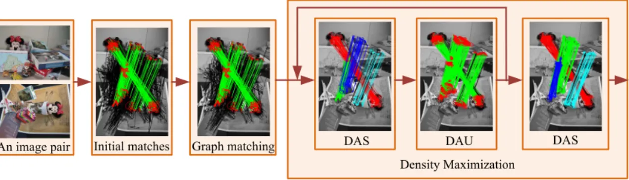
Initial matches Graph matching DAS DAU DAS An image pair

Density Maximization

Figure 1. Overview of our Density Maximization framework. The Graph Matching result contains 283 true matches together with 315 outliers. Density Maximization improves Graph matching by iterating𝐷𝐴𝑆and𝐷𝐴𝑈. 𝐷𝐴𝑆eliminates most outliers and detects four clusters of true matches. 𝐷𝐴𝑈boosts the number of true matches to 416 and introduces only 63 outliers. The final step𝐷𝐴𝑆further removes 19 outliers. True matches are shown with color lines and false matches are shown with black lines.

2.2. Analysis of IQP

Aside from the NP-complete nature, IQP has several other limitations.

Firstly, the combinatorial nature makes the computation

of𝑊 intractable. A real-world image of common size

con-tains more than𝑛= 1000sparse features by using the

pop-ular affine or scale invariant detectors such as SIFT [18], MSER [20] and Harris Affine [21]. This results in a huge

affinity matrix of dimension(𝑛×𝑛)2= 10004. Most graph

matching methods reduces the size of𝑊 by using matches

at a relatively high unary similarity. Such a simple scheme often leads to the loss of useful information hidden in the full matching space [5].

Secondly, IQP prefers more matches. Let 𝑣𝑃_𝑖 and 𝑣𝑄_𝑎

denote two noisy features which have no true matching

ones, setting 𝑋𝑖;𝑎 = 1non-decreases the objective

func-tion 𝑥𝑇𝑊 𝑥because every element of𝑊 is non-negative.

This means that IQP prefers including the matches of all the features, even if they might be outliers. To alleviate this

problem, some methods sparsify𝑥by increasing large

val-ues while smoothing out small valval-ues [2, 8, 14, 23, 11]. The results still contains many outliers.

Finally, IQP assumes that the feature set from one image belongs to a single cluster. This means that the quality of one match is measured based on all current matches. From

(1) we can see that the contribution of each match(𝑣_𝑙𝑃, 𝑣_𝑚𝑄)

to the objective function is

𝐶(𝑙, 𝑚) =𝑥𝑙𝑚( ∑ 𝑖∕=𝑙,𝑎∕=𝑚 𝑊𝑖𝑎;𝑙𝑚𝑥𝑖𝑎+ ∑ 𝑗∕=𝑙,𝑏∕=𝑚 𝑊𝑙𝑚;𝑗𝑏𝑥𝑗𝑏) (2) If 𝐶(𝑙, 𝑚) > 𝐶(𝑙, 𝑠), IQP prefers (𝑣_𝑙𝑃, 𝑣𝑄_𝑚) to(𝑣𝑃_𝑙 , 𝑣_𝑠𝑄),

and vice versa. 𝐶(𝑙, 𝑚) contains the similarities between

(𝑣𝑃

𝑙 , 𝑣𝑄𝑚)and all the other matches. This measure is

prob-lematic for many-to-many object correspondences because the matches in one object correspondence might clutter those in others. To avoid this, each object correspondence

should be considered independently.

3. Density Maximization

Similar to [2, 4, 14, 18], we construct an association

graph 𝐺𝑎𝑔 = (𝑉𝑎𝑔, 𝐸𝑎𝑔, 𝐴𝑎𝑔) based on the affinity

ma-trix𝑊. We take each candidate match(𝑣_𝑖𝑃, 𝑣𝑄_𝑎)as a node

𝑣𝑖𝑎∈𝑉𝑎𝑔, and its associated weight𝑊𝑖𝑎;𝑗𝑏as the attribute

𝑎𝑖𝑎;𝑗𝑏 ∈ 𝐴𝑎𝑔 of the edge 𝑒𝑖𝑎;𝑗𝑏 ∈ 𝐸𝑎𝑔. Then the

origi-nal graph matching problem between𝐺𝑃 and𝐺𝑄becomes

node selection problem in the graph𝐺𝑎𝑔. For brevity, we

will use a single letter to index the node of𝐺𝑎𝑔in the

fol-lowing sections, e.g.,𝑣_𝑖 denotes the𝑖−𝑡ℎnode and𝑊_𝑖;𝑗

denotes the component of𝑊at the𝑖−𝑡ℎrow and the𝑗−𝑡ℎ

column.

Figure 1 shows the framework of Density Maximization. Given an image pair, the salient features are firstly extracted

from each image and then𝑁_𝐶candidate matches are readily

established using unary descriptors of the features at a rela-tively low cost. Those matches are taken as the nodes of an initial association graph. Graph matching selects best nodes from it in order to maximize the objective function in (1). Then a reduced set of nodes and their edges are selectively used to construct a new graph which is called valid graph

𝐺𝑉 _{in this paper. Density Maximization improves}_𝐺𝑉 _by

iterating𝐷𝐴𝑆 and𝐷𝐴𝑈. Based on 𝐺𝑉,𝐷𝐴𝑆 finds the

clusters of nodes as well as removes the outliers by local

maximization of the 𝐷𝐿𝐸 values. 𝐷𝐴𝑈 produces a

up-dated graph𝐺𝑈 with𝑁𝐶nodes by global maximization of

the𝐷𝐿𝐸 values via exploring a much larger graph called

potential graph 𝐺𝑇. At each iteration, the result of𝐷𝐴𝑆

is the starting point of𝐷𝐴𝑈. This ensures that the updates

of matches are mainly based on inliers. The iterations

con-tinue until the total𝐷𝐿𝐸 values no longer increase. The

final step𝐷𝐴𝑆 further removes the outliers introduced by

𝐷𝐴𝑈. As can be seen from Fig.1, Density Maximization is

orthogonal to specific graph matching algorithms, and any 4323

(6)

0 200 400 600 800 0 10 20 30 40 50

node location (width) in the image

DLE Inliers Outliers (a) 0 200 400 600 800 0 5 10 15 20 25

node location (width) in the image

DLE

Inliers Outliers

(b)

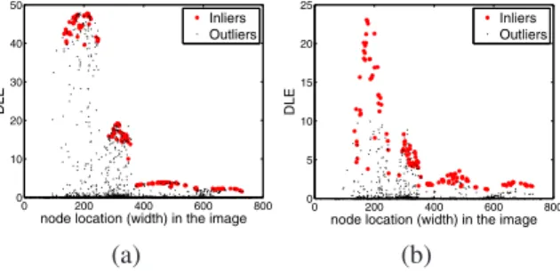
Figure 2. Kernel density estimation for inliers (denoted by red star) and outliers (denoted by black dot). (a) NoΩconstraint. (b) With

Ωconstraint.

of them can be adopted as the graph matching module in the framework.

3.1. Density local estimator

Recently, graph density has shown its potentials to iden-tify inliers and detect strongly connected node clusters in an association graph. A few attempts to define the graph density include the average kernel density of Liu et al.[17], the random walk density of Cho et al.[4], and the personal-ized PageRank density of Cho et al.[3]. Now we define our

density local estimator (𝐷𝐿𝐸). The main difference

be-tween𝐷𝐿𝐸and other methods lies in its well-defined local

smooth domain.

The intuitive of𝐷𝐿𝐸is to estimate graph density at one

node by using only the nodes within a same object, so that it can avoid the clutter problem introduced by outliers and the nodes in other objects. However, it is difficult to determine whether two nodes belong to a same object. Fortunately, it has been observed that the geometric transformations as-sociated with neighbouring matches in a same object are smoothly varying even for significant displacements [16]. This reveals a simple method to approximately identify the nodes within a same object by using a local smooth

neigh-bourhoodΩ. Ω(𝑖)should satisfy two criteria: (1) Locality:

the neighbours are within a close proximity to node𝑣𝑖. (2)

Smoothness: the neighbours should have similar values to

𝑣𝑖 for a same measure. These criteria prevent the scope of

neighbours from extending into outliers and the nodes in other objects.

We adopt the popular kernel density estimation method to compute the graph density locally. We consider node

se-lection as a distribution and use𝑥_𝑖to denote the probability

of selecting node 𝑣_𝑖. Suppose we sample the distribution

𝑁(𝑁 → ∞) times, then the number of selecting𝑣_𝑖is𝑁𝑥_𝑖.

The density at𝑣_𝑖is 𝐷𝐿𝐸(𝑖) = ∑ 𝑗∈Ω(𝑖)𝑁𝑥𝑗𝐾(𝑖, 𝑗) 𝑁 = ∑ 𝑗∈Ω(𝑖) 𝑥𝑗𝐾(𝑖, 𝑗) (3)

This is called𝐷𝐿𝐸in this paper. 𝐾(𝑖, 𝑗) = 𝑊_𝑖;𝑗 implies

1 2 3 4 5 6 7 8 9 10 0 0.1 0.2 0.3 0.4 0.5 0.6 Clusters TDP (a) (b)

Figure 3. (a)Top 10 max TDP values. (b)The clusters for top 10 max TDP values. The match clusters of the four object pairs (de-noted with red, green, blue and cyan lines) have TDP values sig-nificantly larger than those of the false match clusters.

the similarity between 𝑣𝑖 and𝑣𝑗. The only difference

be-tween𝐷𝐿𝐸and the classical kernel density estimation lies

inΩ.

The Locality of𝑣_𝑗with respect to𝑣_𝑖is defined by using

the k-nearest neighbour function𝑘𝑁𝑁(⋅, 𝑘):

𝐿(𝑣𝑖, 𝑣𝑗) = 1 𝑖𝑓 𝑣𝑗∈𝑘𝑁𝑁(𝑣𝑖, 𝑘), 0 𝑜𝑡ℎ𝑒𝑟𝑤𝑖𝑠𝑒.

(4)

The Smoothness of Ω(𝑖)is defined on two measures: the

geometric transformation and the probability of node selec-tion. The Smoothness of geometric transformation between

node𝑣_𝑖and𝑣_𝑗amounts to𝑊_𝑖;𝑗. The Smoothness of

proba-bility is measured by𝑒𝑥𝑝(−(𝑥_𝑖−𝑥_𝑗)2/𝜎2)with a

parame-ter𝜎. ThenΩ(𝑖)is defined as a𝜀−𝑛𝑒𝑖𝑔ℎ𝑏𝑜𝑢𝑟ℎ𝑜𝑜𝑑

Ω(𝑖) ={𝑣𝑗 ∈𝑉𝑉∣Φ(𝑖, 𝑗)> 𝜀}

∪

{𝑣𝑖} (5)

where Φ(𝑖, 𝑗) = 𝐿(𝑣𝑖, 𝑣𝑗)𝑊𝑖,𝑗𝑒𝑥𝑝(−(𝑥𝑖−𝑥𝑗)2/𝜎2)and

the parameter𝜀controls the size ofΩ(𝑖). Figure 2

demon-strates the impact of Ω. With the constraint ofΩ, the

in-liers’𝐷𝐿𝐸 values almost consistently larger than those of

outliers at nearby locations.

The node selection probability𝑥naturally corresponds

to the solutions to (1) since many graph matching methods

solve (1) by relaxing the constraints on𝑥such that its

ele-ments can take real values in [0,1]. In those methods,𝑥can

be viewed as the confidence that the matches are true [14] or as the probability of visits by random walks [2, 13, 4]. In

this paper we consider𝑥as the node selection probability.

For other graph matching methods in which𝑥are integer,

we normalize𝑥to obtain a uniform distribution. Therefore

𝐷𝐿𝐸 is orthogonal to specific graph matching algorithms

whether𝑥are continuous or not, unlike other methods.

3.2. Density Ascent Shift

As shown in Fig.1, the aim of𝐷𝐴𝑆 is to produce node

clusters and eliminate outliers from valid graph𝐺𝑉. 𝐷𝐴𝑆

is a mode-seeking method and the density modes on a graph are defined as follows.

(7)

Algorithm 1: Density Ascent Shift Input: matching(𝐺𝑉, 𝑥)

Output: clean graph𝐺𝐶and an indicator𝐼𝑆for clusters

1 compute𝐷𝐿𝐸(𝑖)∀𝑣𝑖∈𝐺𝑉

2 for each node𝑣𝑖∈𝐺𝑉 do

𝐷𝐴(𝑖) = arg max𝑗∈Ω(𝑖)𝐾(𝑖, 𝑗)Δ𝐷𝐿𝐸(𝑗)

end

3 assign each node𝑣_𝑗to its mode by a tree traversal

along𝐷𝐴(𝑖), and compute the total-density

4 compute the𝑇 𝐷𝑃 for each cluster, and remove

outliers with𝑇 𝐷𝑃 < 𝑡

5 produce final graph𝐺𝐶using the left clusters, set

𝐼𝑆(𝑖) =𝑚if node𝑣𝑖belongs to the𝑚−𝑡ℎcluster

Definition 1Density modes on a graph are local

maxi-mizers of the𝐷𝐿𝐸values.

𝐷𝐴𝑆 performs mode-seeking along the density-ascent

direction. The density-ascent𝐷𝐴(𝑖)of node𝑣_𝑖 is

formu-lated as

𝐷𝐴(𝑖) = arg max

𝑗∈Ω(𝑖)𝐾(𝑖, 𝑗)Δ𝐷𝐿𝐸(𝑗) (6)

which means the neighbouring node of 𝑣𝑖 with the

high-est expectation of𝐷𝐿𝐸 increment. This density-ascent is

the steepest ascent over the𝐷𝐿𝐸values withinΩ(𝑖).Ω(𝑖)

prevents shifting into irrelevant clusters. Similar to other

mode-seeking methods[12, 4, 3], 𝐷𝐴𝑆 is guaranteed to

converge.

Theorem 1 A finite sequence of density-ascent shifts from any node converges to a density mode.

ProofSinceΩ(𝑖)of any node𝑣_𝑖includes itself, the𝐷𝐿𝐸 values of a sequence of shifts keep strictly increasing until the shifts reach a node whose density-ascent is itself. The final node, therefore, is the density mode, and the length

of the sequence is ∣𝑉𝑉∣at most, with ∣𝑉𝑉∣denoting the

number of nodes in𝐺𝑉.

For each node, we compute its density-ascent just once. Then the successive density-ascent for any node already ex-ists. The trajectory of nodes sharing a common density mode builds a tree, and leads to a natural cluster. Then the cluster label of all nodes associated with each disjoint tree can be assigned in a single tree traversal, similar to the medoid shift[22].

We define the total-density of each cluster as the sum

of the𝐷𝐿𝐸 values of its members, and the

total-density-percentage (𝑇 𝐷𝑃) of each cluster as the ratio between its

total-density and the sum of the total-densities of all the clusters. The clusters of outliers usually have very small

total-density, so that𝑇 𝐷𝑃 provides a reliable measure for

detection and elimination of them, as shown in Fig.3.𝐷𝐴𝑆

is depicted in Algorithm 1.

Algorithm 2: Density Ascent Update

Input: potential graph𝐺𝑇, clean graph𝐺𝐶,𝑥and𝑁𝐶

Output: a updated graph𝐺𝑈

1 𝑛𝑥(𝑖)←0,𝑑𝑥(𝑖)←0,∀𝑣𝑖 ∈𝐺𝑇

for each node𝑣𝑗 ∈𝐺𝐶do

for each𝑣𝑖∈Ω′(𝑗)do 𝑛𝑥(𝑖)←𝑛𝑥(𝑖) +𝑥𝑗𝐾(𝑗, 𝑖) 𝑑𝑥(𝑖)←𝑑𝑥(𝑖) +𝐾(𝑗, 𝑖) end end 𝑥←𝑛𝑥./𝑑𝑥 2 𝐷𝐿𝐸(𝑖)←0,∀𝑣_𝑖∈𝐺𝑇

for each node𝑣_𝑗 ∈𝐺𝐶do

for each𝑣_𝑖∈Ω(𝑗)do

𝐷𝐿𝐸(𝑖)←𝐷𝐿𝐸(𝑖) +𝑥𝑗𝐾(𝑗, 𝑖)

end end

3 𝐺𝑈 ←𝑁_𝐶nodes with the largest𝐷𝐿𝐸values

3.3. Density Ascent Update

Given a clean graph𝐺𝐶, the aim of𝐷𝐴𝑈is to produce a

updated graph𝐺𝑈 with𝑁_𝐶nodes by maximizing the total

𝐷𝐿𝐸values. To achieve this,𝐷𝐴𝑈 explores the potential

graph𝐺𝑇 which contains𝐺𝐶but is much larger.𝐺𝑇covers

most true matches and will be detailed later. 𝐷𝐴𝑈 firstly

estimates the 𝐷𝐿𝐸 values of the nodes in 𝐺𝑇, and then

select𝑁_𝐶 best nodes with largest values to construct𝐺𝑈.

since𝐺𝐶 ⊂𝐺𝑇, this global maximization scheme ensures

that𝐷𝐴𝑈 non-decreases the total𝐷𝐿𝐸values.

To compute the𝐷𝐿𝐸value for each node𝑣_𝑖in𝐺𝑇, we

need to identifyΩ(𝑖)at first. But the node selection

proba-bility𝑥𝑖might be unavailable if𝑣𝑖does not belong to𝐺𝐶.

Here we approximate𝑥𝑖by 𝑥𝑖= ∑ 𝑗∈Ω′_(𝑖)𝑥𝑗𝐾(𝑖, 𝑗) ∑ 𝑗∈Ω′_(𝑖)𝐾(𝑖, 𝑗) (7) which is a weighted average of the selection

probabil-ities over a local smooth neighbourhood Ω′(𝑖). Ω′(𝑖)

is similar to Ω(𝑖) but does not consider the

probabil-ity Smoothness since 𝑥_𝑖 is unknown. However, 𝑥_𝑗 for

𝑗 ∈ Ω′₍_𝑖₎ _{might be unavailable. We observe that} _Ω′₍_𝑖₎

is nearly symmetric for true matches. By

investigat-ing the nodes for true matches in Fig.1 we find that

if 𝑗 ∈ Ω′(𝑖) the probability for 𝑖 ∈ Ω′(𝑗) is above

90%. Therefore (7) can be approximately rewritten as

𝑥𝑖 = ∑𝑖∈Ω′_(𝑗)𝑥𝑗𝐾(𝑗, 𝑖)/∑𝑖∈Ω′_(𝑗)𝐾(𝑗, 𝑖). Let𝑛𝑥(𝑖) =

∑

𝑖∈Ω′_(𝑗)𝑥𝑗𝐾(𝑗, 𝑖)and𝑑𝑥(𝑖) =∑𝑖∈Ω′_(𝑗)𝐾(𝑗, 𝑖), the

con-tribution of each node𝑣_𝑗 in𝐺𝐶 to𝑛𝑥(𝑖)is𝑥_𝑗𝐾(𝑗, 𝑖), and

that to𝑑𝑥(𝑖)is𝐾(𝑗, 𝑖)if𝑖∈Ω′(𝑗). Therefore all𝑥_𝑖can be

estimated very efficiently by traversing the nodes of𝐺𝐶.

SinceΩ′(𝑖)is nearly symmetric,Ω(𝑖)is also nearly

sym-metric because𝑒𝑥𝑝(−(𝑥_𝑖−𝑥_𝑗)2/𝜎2)is symmetric. Then

(8)

(3) can be rewritten as 𝐷𝐿𝐸(𝑖) = ∑_𝑖_∈_Ω(𝑗)𝑥𝑗𝐾(𝑗, 𝑖)

which means that the contribution of each node𝑣_𝑗 in𝐺𝐶

to𝐷𝐿𝐸(𝑖)is𝑥𝑗𝐾(𝑗, 𝑖). Therefore all𝐷𝐿𝐸(𝑖)can be

effi-ciently calculated by traversing the nodes of𝐺𝐶. 𝐷𝐴𝑈 is

summarized in Algorithm 2.

The potential graph𝐺𝑇 is constructed using𝑍 matches

for each feature based on the unary similarity. We test on the image pairs of the intra-class dataset[1] which own large

intra-category variations, and find that𝐺𝑇covers more than

95%true matches when𝑍= 40. This reveals that exploring

the whole matching space like Cho et al.[5] is unnecessary.

3.4. Analysis

Using the approximate nearest neighbour (ANN)

search, the computational complexity of 𝐷𝐴𝑈 is

𝑂(𝑘∣𝑉𝑉_∣_log(_𝑍𝑛𝑃₎₎ _with _∣_𝑉𝑉_∣ _denoting _the _node

number of 𝐺𝑉, 𝑛𝑃 denoting the node number of graph

𝐺𝑃 _{(i.e., the feature number of one image) and} _𝑘 _{= 50}_.

As far as we know, the only work similar to𝐷𝐴𝑈 is the

progression method[5] whose computational complexity is

𝑂(𝑘1𝑘2∣𝑉𝑉∣log(𝑛𝑃) log(𝑛𝑄))with𝑘1 = 25and𝑘2 = 5.

𝐷𝐴𝑈 is more than one order of magnitude faster because

𝑘1𝑘2log(𝑛𝑃)𝑙𝑜𝑔(𝑛𝑄)/𝑘log(𝑍𝑛𝑃) >10for general cases

with𝑛𝑃 >1000and𝑛𝑄 > 1000. The main difference is

that𝐷𝐴𝑈 explores the potential graph𝐺𝑇 while the

pro-gression method searches the whole matching space based

on 𝐺𝑉. Since 𝐺𝑇 covers most true matches, exploring

𝐺𝑇 _{does not degrade the performance. On the other hand,}

this scheme successfully avoids many outliers in the whole matching space, as will be shown in the experiments.

The computational complexity of 𝐷𝐴𝑆 is

𝑂(𝑘∣𝑉𝑉_∣_log_∣_𝑉𝑉_∣₎_{, more than one order of}

magni-tude faster than most mode-seeking methods. The high

efficiency benefits from its non-iteration scheme. More

importantly, either 𝐷𝐴𝑈 or 𝐷𝐴𝑆 is much faster than

most graph matching methods [2, 8, 14, 15, 23, 19, 11], indicating that we can improve graph matching without introducing too much computational cost.

An important trick of our Density Maximization

frame-work is that 𝐷𝐴𝑈 takes the result of 𝐷𝐴𝑆 as its

start-ing point at each iteration. This ensures that the updatstart-ing matches is mainly based on inliers. In this way, Density Maximization significantly increases the precision in sharp contrast with the progression method, as shown in Fig.4.

4. Experiments

In our experiments, the candidate matches are generated using the SIFT descriptor. To measure the similarity be-tween two matches(𝑣𝑃_𝑖 , 𝑣_𝑎𝑄)and(𝑣_𝑗𝑃, 𝑣𝑄_𝑏), we adopted the

symmetric transfer error𝑑(𝑖𝑎;𝑗𝑏)used in [5, 13, 1, 4]. The

affinity matrix 𝑊 is calculated by𝑊_{𝑖𝑎;𝑖𝑏} = 𝑚𝑎𝑥(50−

𝑑(𝑖𝑎;𝑗𝑏),0). In Density Maximization, we set𝜎 = 0.2,

𝑘= 50,𝜀= 10and𝑡= 0.03. 0 2 4 6 8 0.4 0.5 0.6 0.7 0.8 0.9 1 Iterations Precision Density Maximization Progression

Figure 4. Performance growth on the image pair in Fig.1 by our Density Maximization and the progression method[5]. The plot shows the precision w.r.t the iteration steps. Note that the step 0 denotes the result by graph matching.

(a) (b) (c) (d)

Figure 5. (a)The result by GP[5] based on the graph matching re-sult in Fig.1. (b)The rere-sult by our𝐷𝐴𝑈. (c)The result by GP together with our𝐷𝐴𝑆. The false match clusters are denoted by yellow and magenta lines. (d)The result by our 𝐷𝐴𝑈 together with our𝐷𝐴𝑆. There is no false match clusters.

We test Density Maximization on three challenging

benchmark datasets: Intra-class dataset[1], ETHZ toys

dataset[10], Co-recognition dataset[6]. Intra-class dataset consists of 30 image pairs of large transformations and intra-class variation. It provides detected MSER features and initial matches. In this dataset, most images have a small number of features and only several hundreds of ini-tial matches. For fair comparison, we adopt those features

and always fix the number of candidate matches𝑁_𝐶 to the

same as the number of the given initial matches. ETHZ toys dataset includes 9 different rigid/non-rigid objects together with the test images of significant clutter. Co-recognition dataset contains 6 image pairs with complex many-to-many object correspondences. The ground truth feature correpon-dences are manually constructed for each image pairs to en-able quantitatively evaluation. For these two dataset, we use the MSER and the Harris affine detectors with the SIFT

de-scriptor, and set 𝑁_𝐶 = 3000. Our testing environment is

MS Windows 7 Professional with Intel Core i5-3550 CPU 3.3GHz, 16GB RAM.

4.1. Density Maximization vs related work

Density Maximization contains novel approaches to both

updating matches (i.e.,𝐷𝐴𝑈) and clustering matches (i.e.,

(9)

(a) (b)

(c) (d)

Figure 6. (a)A image pair. (b)The result by SAE[17]. (c)The result by (ACC)[1]. (d)The result by our𝐷𝐴𝑆. True matches are shown with green lines and false matches are shown with black lines.

D PG 𝐷𝐴𝑈 ACC SAE 𝐷𝐴𝑆 PG+ DM

ACC

1 81 83 71 43 83 71/70 73/81

2 69 77 63 No 85 62/69 72/88

3 66 81 67 No 91 61/74 75/92

Table 1. Recall (%) of PG and our 𝐷𝐴𝑈, Precision (%) of ACC, SAE and our𝐷𝐴𝑆, Recall/Precision (%) of PG+ACC and our Density Maximization (DM). D 1,2 and 3 denote Intra-class dataset, ETHZ toys dataset and Co-recognition dataset respec-tively. ’No’ denotes the failure of SAE.

steps as well as a whole.

Firstly we compare our 𝐷𝐴𝑈 with the graph

progres-sion (GP)[5] since it is the only similar work to𝐷𝐴𝑈as far

as we know. For fair comparison, we adopt the same pro-gressive framework as GP, which performs graph matching and updating matches iteratively. Since the aims of both

𝐷𝐴𝑈 and GP are to boost the true matches, we access

Re-call on the three datasets. The results of GP contain lots of overlapping matches. To compute Recall more accurately, we count the overlapping matches only once. The overall

results are given in Table 1. Compared to our𝐷𝐴𝑈, GP

tends to introduce more outliers which are very difficult to remove. Figure 5 shows the outliers of an example. The av-erage times for each iteration of GP to process each image pair in the three data-sets are 0.45, 5.32 and 31.53 seconds

respectively. The corresponding times for𝐷𝐴𝑈 are 0.27,

1.64 and 3.73 seconds respectively.

Secondly, we compare our𝐷𝐴𝑆 with two

state-of-the-arts methods: the agglomerative correspondence clustering (ACC)[1] and the Shrink-and-Expansion (SAE)[17]. Since SAE cannot handle both ETHZ toys and Co-recognition datasets (the source code provided by the authors on the internet has ’out of memory’ problem when handling thou-sands of matches), we only report its result for Intra-class

dataset. Since the aim of𝐷𝐴𝑆is to improve Precision, we

access Precision on the three datasets. The overall results are given in Table 1 and an example is shown in Fig.6. SAE

(a) (b)

(c) (d)

Figure 7. (a)A image pair. (b)Graph matching result. (c)The result by GP+ACC. (d)The result by our Density Maximization. True matches are shown with green lines and false matches are shown with black lines.

D SM PM BGM IPFP RRWM

1 43/47 39/44 32/36 47/39 45/41

2 23/64 27/52 18/45 33/67 29/53

3 27/51 25/49 21/42 33/41 31/44

Table 2. Performance improvement (%) over Recall/Precision by Density Maximization.

tends to include lots of outliers. The results of ACC are

much better, but are still noisy. In contrast, our𝐷𝐴𝑆

suc-cessfully detects true matches and distinguishes them from outliers. To process each image pair in the three datasets

𝐷𝐴𝑆 takes only 0.69, 1.72 and 1.93 seconds on average,

while ACC takes 8.74, 78.52 and 95.73 seconds. SAE is much slower and takes more than one minute on average to process each image pair of Intra-class dataset.

Finally, we compare our Density Maximization with a combined method—GP+ACC. GP+ACC is performed in a similar way of Density Maximization: GP and ACC are per-formed iteratively till convergence. We measure both Recall and Precision on the three datasets. As shown in Fig.7, the outliers introduced by GP cannot be eliminated by ACC, and result in noisy clusters. So GP+ACC increases Recall at the expense of Precision. Our Density Maximization solves this problem effectively by avoiding outliers from source. It largely outperforms GP+ACC in both precision and recall as shown by Table 1.

4.2. Density Maximization vs Graph Matching

In this experiment, we show the improvement of Den-sity Maximization on several state-of-the arts graph match-ing methods: SM[14], PM[24], BGM[8], IPFP[15] and RRWM[2]. The quantitative results are summarized in Ta-ble 2, and some examples are shown in Fig.8. The graph matching methods cannot distinguish inliers from outliers, and fail to separate matches of one object from those of others. Density Maximization solves these problems effec-tively by detecting clusters of true matches. The precision 4327

(10)

(a) (b)

(c) (d)

(e) (f)

Figure 8. (a) and (b) are two input image pairs. (c)Result by RRWM[2] for (a). (d)Result by SM[2] for (b). (e)The result by our Density Maximization with RRWM as the graph matching mod-ule. (f)The result by our Density Maximization with SM as the graph matching module. True matches are shown with color lines and false matches are shown with black lines.

is boosted by36%∼67%, and the recall by18%∼47%.

5. Conclusion

We introduced a unified framework, called Density Max-imization, which effectively resolves the three limitations of conventional graph matching and achieves impressive per-formance improvement. By globally and locally maximiz-ing a novel proposed density estimator, i.e., density local estimator, Density Maximization leads to the integration of updating matches, eliminating outliers and cluster detec-tion. We point out that the key to the high performance is twofold: a well-defined local smooth neighbourhood to avoid clutter and an iteration scheme to ensure that updating matches is mainly based on inliers. Experiments demon-strate that Density Maximization is adequate for very chal-lenging real-world images which contain many-to-many ob-ject correspondences and significant outliers.

6. Acknowledgement

This work is supported by Australian Research Council (ARC) Linkage Grant LP0991757.

References

[1] M. Cho, J. Lee, and K. M. Lee. Feature correspondence and deformable object matching via agglomerative correspon-dence clustering.ICCV, 2009.

[2] M. Cho, J. Lee, and K. M. Lee. Reweighted random walks for graph matching.ECCV, 2010.

[3] M. Cho and K. M. Lee. Authority-shift clustering: Hier-archical clustering by authority seeking on graphs. CVPR, 2010.

[4] M. Cho and K. M. Lee. Mode-seeking on graphs via ran-domwalks.CVPR, 2012.

[5] M. Cho and K. M. Lee. Progressive graph matching: Making a move of graphs via probabilistic voting.CVPR, 2012. [6] M. Cho, Y. M. Shin, and K. M. Lee. Co-recognition of image

pairs by data-driven monte carlo image exploration. ECCV, 2008.

[7] D. Conte, P. Foggia, C. Sansone, and M. Vento. Thirty years of graph matching in pattern recognition. IJPRAI, pages 265–298, 2004.

[8] T. Cour, P. Srinivasan, and J. Shi. Balanced graph matching.

NIPS, 2007.

[9] O. Duchenne, F. Bach, I. Kweon, and J. Ponce. A tensor-based algorithm for high-order graph matching. CVPR, 2009.

[10] V. Ferrari, T. Tuytelaars, and L. V. Gool. Simultaneous object recognition and segmentation from single or multiple model views.IJCV, 67(2):159–188, 2006.

[11] M. Gori, M. Maggini, and L. Sarti. Exact and approximate graph matching using random walks. TPAMI, 27(7):1100– 1111, 2005.

[12] S. Jouili, S. Tabbone, and V. Lacroix. Median graph shift: A new clustering algorithm for graph domain.ICPR, 2010. [13] J. Lee, M. Cho, and K. M. Lee. Hyper-graph matching via

reweighted random walks.CVPR, 2011.

[14] M. Leordeanu and M. Hebert. A spectral technique for corre-spondence problems using pairwise constraints.ICCV, 2005. [15] M. Leordeanu and M. Herbert. An integer projected fixed point method for graph matching and map inference. NIPS, 2009.

[16] W. Lin, S. Liu, Y. Matsushita, and T. Ng. Smoothly varying affine stitching.CVPR, 2011.

[17] H. Liu, L. J. Latecki, and S. Yan. Fast detection of dense subgraph with iterative shrinking and expansion. TPAMI, 2013.

[18] D. G. Lowe. Object recognition from local scale-invariant features.ICCV, 1999.

[19] J. Maciel and J. Costeira. A global solution to sparse corre-spondence problems.TPAMI, 25(2):187–199, 2003. [20] J. Matas, O. Chum, M. Urban, and T. Pajdla. Robust

wide baseline stereo from maximally stable extremal re-gions.BMVC, 2002.

[21] K. Mikolajczyk and C. Schmid. Scale and affine invariant interest point detectors.IJCV, 2004.

[22] Y. A. Sheikh, E. A. Khan, and T. Kanade. Mode-seeking by medoid shifts.ICCV, 2007.

[23] L. Torresani, V. Kolmogorov, and C. Rother. Feature corre-spondence via graph matching: Models and global optimiza-tion.ECCV, 2008.

[24] R. Zass and A. Shashua. Probabilistic graph and hypergraph matching.CVPR, 2008.

[25] W. Zhang, X. Wang, D. Zhao, and X. Tang. Graph de-gree linkage: agglomerative clustering on a directed graph.