Likelihoods
Zhaoshi Meng∗ Dennis Wei∗ Ami Wiesel† Alfred O. Hero III∗
∗University of Michigan
{mengzs,dlwei,hero}@eecs.umich.edu
†The Hebrew University of Jerusalem [email protected]
Abstract
We consider distributed estimation of the inverse covariance matrix, also called the concentration matrix, in Gaussian graphical models. Traditional centralized estimation often requires iterative and expensive global inference and is therefore difficult in large dis-tributed networks. In this paper, we propose a general framework for distributed estima-tion based on a maximum marginal likeli-hood (MML) approach. Each node indepen-dently computes a local estimate by maximiz-ing a marginal likelihood defined with respect to data collected from its local neighbor-hood. Due to the non-convexity of the MML problem, we derive and consider solving a convex relaxation. The local estimates are then combined into a global estimate with-out the need for iterative message-passing be-tween neighborhoods. We prove that this re-laxed MML estimator is asymptotically con-sistent. Through numerical experiments on several synthetic and real-world data sets, we demonstrate that the two-hop version of the proposed estimator is significantly better than the one-hop version, and nearly closes the gap to the centralized maximum likeli-hood estimator in many situations.
1
Introduction
Graphical models provide a principled framework for compactly representing dependencies among random variables (Lauritzen, 1996; Wainwright & Jordan, 2008). The ability to perform distributed and effi-cient inference makes them especially well-suited to Appearing in Proceedings of the 16th International
Con-ference on Artificial Intelligence and Statistics (AISTATS) 2013, Scottsdale, AZ, USA. Volume 31 of JMLR: W&CP 31. Copyright 2013 by the authors.
large networks,e.g., sensor networks, social networks, gene regulatory networks, and smart grids (Liu & Ih-ler, 2012; Meng et al., 2012; Wiesel & Hero, 2012). Estimating graphical model parameters is therefore an important first step in enabling these applications. For Gaussian graphical models (GGM), parameter es-timation essentially reduces to covariance eses-timation and is further simplified by the graph structure: the pattern of edges in the graph corresponds to the spar-sity pattern of the inverse covariance matrix, also known as the concentration or precision matrix. When the sparsity pattern is known a priori, the traditional technique for inverse covariance estimation is maxi-mum likelihood (ML), resulting in a convex optimiza-tion that can be solved either by generic solvers or spe-cialized algorithms (Banerjee et al., 2006; Dahl et al., 2008; Friedman et al., 2008). However, solving the exact ML estimation problem requires either expen-sive data communication (e.g., to a fusion center) and centralized computation/storage, or in a distributed setting, iterative message-passing in loopy graphs to compute global derivatives (Koller & Friedman, 2009). Neither of those strategies are feasible in large, gener-ally structured and distributed networks, such as a sen-sor network where the corresponding graph could be very loopy and the computational resources are highly decentralized.
Given the limitations of centralized solutions, re-searchers have begun proposing distributed methods for graphical model learning, where agents in the net-work estimate local parameters by processing local data with limited communication between agents (Liu & Ihler, 2012; Wiesel & Hero, 2012). In addition to decentralizing computation and communication across the network, distributed solutions are naturally robust against localized attacks or failures, and are also more protective of data privacy. These advantages make dis-tributed algorithms particularly appealing for network applications.
This paper proposes a general framework for dis-tributed estimation based on marginal likelihoods.
Each node collects data within its neighborhood and independently forms a local estimate by maximizing a marginal likelihood. We show that this marginal likelihood approach is sufficient in principle to deter-mine the global parameter. Notably, the formation of our global estimate from local estimates does not re-quire iterative consensus or message-passing as in Liu & Ihler (2012); Wiesel & Hero (2012). Due to the non-convexity of maximum marginal likelihood (MML) es-timation, we derive and consider solving a convex re-laxation of the problem. We prove that the relaxed MML estimator is asymptotically consistent. We then focus on two specific cases in which the local neigh-borhoods correspond to either one or two communica-tion hops through the network. Extensive experiments show that the two-hop version of the proposed estima-tor is significantly better than the one-hop version and nearly closes the gap to the centralized ML estimator in many situations.
The outline of the paper is as follows. In Section 2, we give a brief review of graphical models and centralized ML estimation. In Section 3, we propose a general approach to distributed estimation based on marginal likelihoods, show asymptotic consistency, and discuss two important specific cases. Numerical experiments are presented in Section 4 and the paper concludes in Section 5.
1.1 Related work
Recent works by Liu & Ihler (2012); Wiesel & Hero (2012) have discussed a similar but less general framework for distributed estimation in which sev-eral pseudo-likelihood-based estimators for GGMs and general exponential families are proposed. In Section 3.4, we show that the estimators in Wiesel & Hero (2012) can be seen as a special case of the proposed relaxed MML estimator, and a significant performance improvement can be obtained through a reasonable in-crease in the computation and communication cost. Our distributed estimator is formed through solving multiple relaxed MML estimation problems by local agents. The structure of each local MML problem is related to the latent graphical model considered in Chandrasekaran et al. (2012). However, the as-sumption in Chandrasekaran et al. (2012) is that the number of latent variables is relatively small, thus con-tributing a low-rank term, whereas in our case, all vari-ables outside the local neighborhood can be seen as latent variables.
Another line of work (Friedman et al., 2008; Johnson et al., 2011; Ravikumar et al., 2011; Rothman et al., 2008) focuses on the problem of covariance selection, where the graph topology is not known a priori and
must be estimated in addition to the parameters. This appears to be a harder problem than ours since we as-sume the structure is known, but some insights regard-ing distributed algorithms in particular can perhaps be shared.
Notation. Boldface upper case letters denote ma-trices and boldface lower case letters denote column vectors. Sets of single indices are denoted by calli-graphic upper case letters. The cardinality of a setA
is denoted by|A| and the difference of two sets is de-noted as A\B. Following common notation, AM,N represents a submatrix of A with rows indexed by
M and columns indexed by N. We also make ref-erence to irregular sets of index pairs such as the edge set E of a graph, for which we use standard upper case letters. AE then refers to the vector of entries of A indexed by E. The standard inner product be-tween two symmetric matrices is denoted as hA,Bi, i.e., hA,Bi= trace(AB) =P
i,jAi,jBi,j.
2
Background
2.1 Graphical models
We refer the reader to Lauritzen (1996) for a de-tailed treatment of graphical models. We consider a
p-dimensional random vector x following a graphical model with respect to an undirected graphG= (V, E), where V ={1, . . . , p} is a set of nodes corresponding to elements of x and E is a set of edges connecting nodes. The vector x satisfies the Markov property with respect to Gif for any pair of nonadjacent nodes in G, the corresponding pair of variables inxare con-ditionally independent given the remaining variables. For Gaussian graphical models (GGM), the vector x follows a multivariate Gaussian distribution. We as-sume without loss of generality thatxhas zero mean. Then the probability density function can be written in canonical form in terms of the concentration matrix Jas follows: p(x;J) = (2π)−p/2(detJ)1/2exp −1 2x TJx . (1)
The Markov property manifests itself in a simple way through the sparsity pattern of J:
Ji,j= 0 for all (i, j)∈/ E. (2) This property leads to efficient inference algorithms for GGMs, and as we will show, it can also be exploited for distributed parameter learning.
2.2 Centralized estimation in GGMs
Maximum likelihood estimation (MLE) is a classical approach to estimating model parameters from data.
For Gaussian graphical models, the problem reduces to estimating the non-zero elements of the concentra-tion matrix J. These elements are indexed by Ee, the
union of the edges and pairs corresponding to diagonal elements,
e
E:=E∪ {(i, i)}pi=1. (3) When all the data are accessible, the centralized global maximum likelihood (GML) estimation problem can be formulated as Lauritzen (1996) b JGML= arg min J hΣb,Ji −log detJ s.t. Jj,k= 0 ∀(j, k)∈/E,e J0. (4) where Σb = T1 PT t=1x(t)x(t)
T is the sample covari-ance matrix and x(1), . . . ,x(T) are i.i.d. samples of x. Since the GML problem (4) is convex in J
e E, effi-cient gradient-based algorithms can be applied, many of which have specialized implementations on graphs,
e.g.iterative proportional fitting (IPF) (Wainwright & Jordan, 2008), chordally-embedded Newton’s method (Dahl et al., 2008), and an iterative regression method introduced in Friedman et al. (2009). However, as mentioned before, the main drawback of these methods is the computational and communication complexity when implemented in networks.
3
Distributed Estimation in GGMs
We now consider a general approach to distributed parameter estimation motivated by network applica-tions. Each random variable xi is associated with a node in the network. The topology of the graph G, which encodes statistical dependences, is assumed to coincide with the topology of internode communica-tion. Each node collects all the data samples from within a neighborhood and computes a local parame-ter estimate. A global estimate ofJis then formed by combining these local estimates. The key components in this framework are the choice of neighborhood, the local estimation method, and the method for combin-ing estimates.
3.1 Marginal Likelihood Maximization In this paper, we propose to estimate local parameters by maximizingmarginal likelihood functions. For each nodei, define the index set for itsimmediate neighbors
as
Ii:={j |(i, j)∈E}, (5) and consider a neighborhood indexed by a setNi con-taining the nodes within a certain number of communi-cation hops from nodeiin the network. By definition,
the set Ni includes at least the node i itself and its immediate neighbors Ii. LetK denote the concentra-tion matrix corresponding to the marginal distribuconcentra-tion over the variables {xj, j ∈ Ni} in the neighborhood, and let Si:=ΣNb i,Ni = 1 T T X t=1 xNi(t)xNi(t)T
be the local sample covariance matrix. Then the max-imum marginal likelihood (MML) estimation problem in neighborhoodNi can be formulated as a joint opti-mization of KandJ: b Ki,MML= arg min K,J hSi,Ki −log detK s.t. K=h J−1N i,Ni i−1 , Jj,k= 0 ∀(j, k)∈/ E,e J0, (6)
where the first constraint represents the marginaliza-tion relamarginaliza-tionship betweenKandJand the second line of constraints reflects the sparsity of the global param-eter.
A global estimate of J can be formed by combining optimal solutions to problem (6) for each node i. We consider a simple concatenation approach whose justi-fication will be given in Section 3.2 below. Denote by
Lithe set of index pairs corresponding to the non-zero entries in theith row ofJ, i.e.,
Li :={(j, k)∈Ee |j=i}. (7)
Note that the self-edge pair (i, i) is included inLigiven the definition of Ee in (3). We refer to the parameters
indexed by Li as therow parameters for node i. The global estimate is constructed by extracting the row parameters from each local estimate and concatenat-ing them: b JMMLL i =Kb i,MML Li , fori= 1, . . . , p. (8)
Note that this construction of the global estimate JMML (and also the other surrogate estimator pro-posed below) does not guarantee symmetry, since it is not a major concern of this work. However, as will shown in Section 3.3, the symmetry is naturally recov-ered in the asymptotic limit; also it can be imposed in the non-asymptotic case through a simple strategy (see Section 3.6).
The difficulty with the MML approach is that prob-lem (6) is in general a non-convex optimization. The non-convexity arises from the coupling of the nonlinear marginalization constraint linkingKtoJand the spar-sity constraints onJ. In the next subsection, we derive a convex relaxation of the MML estimation problem as a surrogate.
i
(a) 2D lattice and two-hop neighbor-hood
i
(b) A general graph and two-hop neighborhood
i i
(c) Local relaxations (one-hop (left) and two-hop (right))
Figure 1: Illustration of defined sets and local relaxation. In (a) and (b) we show two different graphs, in which the two-hop neighborhood N for nodei is indicated with dashed contours. The buffer set variablesxBand the protected set variablesxP (excluding nodeiitself) are colored blue and red, respectively. For the graph in (b), we illustrate the one-hop and two-hop local relaxation problems in (c). The dashed red lines in (c) denote the fill-in edges due to relaxation.
3.2 Convex Relaxation of Marginal Likelihood Maximization
In the remainder of the section, we suppress the node index iwhenever possible for clarity. To derive a con-vex relaxation of the MML estimation problem (6), we apply the Schur complement identity to the marginal-ization constraint in (6), yielding
K=JN,N −JN,NC ·
JNC,NC −1
·JNC,N, (9)
whereNC is the complementary set toN. Define the
buffer set B ⊂ N as the set of all variables inN that have immediate neighbors in the complementNC,
B:={j |j∈ N andIj∩ NC 6=∅}. (10)
The difference set between N and Bis referred to as theprotected set P :=N \B. The buffer and protected sets are illustrated in Figure 1(a) and 1(b). Due to the Markov property, we have JP,NC = 0. Decomposing
N into B and P then reveals the sparsity pattern of K from (9): K=JN,N − 0 JB,NC JNC,NC −1 0, JNC,B =JN,N − 0 0 0 JB,NC JNC,NC −1 JNC,B and hence KP,P =JP,P, KP,B=JP,B, (11) KB,B=JB,B−JB,NCJNC,NC −1 JNC,B. (12)
An important observation from (11) is that the spar-sity pattern of JN,N is entirely preserved in the rows
and columns indexed by the protected set P. In par-ticular, because node i itself is always protected, the marginal and global concentration matrices share the same values of the row parameters indexed byL, which motivates our strategy for fusing local estimates in (8). On the other hand, the sparsity pattern in the “buffer submatrix”KB,Bis in general modified due to the fill-in term, i.e., the second term in (12).
Based on these observations, we now specify a relaxed set of constraints on the marginal concentration matrix K. First denote the set of all local edges that are not affected by the fill-in term in (12) as
EProt:=Ee∩ {{P × P} ∪ {P × B} ∪ {B × P}},
where the superscript stands for “protected”. We then add toEProtall index pairsB×Bthat could potentially
be affected by fill-in in (12), resulting in arelaxed edge set R(see Figure 1(c) for illustrations):
R=EProt∪ {B × B}. (13) In light of (11) and (12), any feasible marginal con-centration matrixKfor the MML estimation problem (6) is guaranteed to be supported only on the set R. Therefore the following constraints specify a set that contains the feasible set of the MML problem (6):
K0andKj,k= 0 ∀(j, k)∈/ R. (14) Using the constraints in (14), we formulate the follow-ing relaxation of the original MML estimation problem (6) at each nodei:
b
Ki,Relax= arg min
K
hSi,Ki −log detK s.t. Kj,k= 0 ∀(j, k)∈/R,
K0.
The above relaxed MML problem is a convex opti-mization with respect to KR and has the same form as the global MLE problem (4) but with much lower dimensions in general.
Since the original MML estimation problem (6) is dif-ficult to solve, we propose to solve the relaxed MML estimation problem (15) as a surrogate to estimate the local parameters. Then a global estimate of the con-centration matrix can be similarly obtained by extract-ing and concatenatextract-ing row parameters as in (8):
b JRelaxL i =Kb i,Relax Li , fori= 1, . . . , p. (16) 3.3 Asymptotic Consistency
In this section, we suppress the indexifor matricesS andKRelaxfor clarity. We prove that the relaxed MML
estimator defined in (15) and (16) is asymptotically consistent. To do so, we first establish the following lemma by making use of the continuity of the mapping from sample covariance Sto local estimateKbRelax in
(15) (proof omitted).
Lemma 1. The mapping from the sample covariance
S to the concentration matrix KbRelax through solving
the relaxed MML problem (15) is a continuous map-ping provided that Sis positive definite.
Theorem 1. The relaxed MML estimator bJRelax is
asymptotically consistent.
Proof of Theorem 1. In the asymptotic limit, the lo-cal sample covariance matrix Sconverges to the cor-responding sub-matrix of the true covariance matrix, Σ∗N,N, with probability one and is therefore positive definite. Let K∗ = (Σ∗N,N)−1 be the corresponding
true marginal concentration matrix. We first show that K∗ is the optimal solution to the relaxed MML estimation problem (15) whenS=Σ∗N,N. To see this, note that the true global concentration matrixJ∗ con-forms to the sparsity pattern specified byEe, and
there-fore the marginal concentration matrix K∗ is feasible for (6). Furthermore, from relations (11)-(12) and our construction of the edge set R, K∗ also satisfies the sparsity constraints of the relaxed problem (15). It is straightforward to show that K∗ satisfies the opti-mality conditions when S = Σ∗
N,N. Then by strict convexity, K∗ is the unique optimum of the relaxed MML problem whenS=Σ∗N,N.
It now follows from Lemma 1 and the continuous mapping theorem (Van der Vaart, 2000) that the re-laxed MML estimates KbRelaxconverge asymptotically
to K∗ with probability one. Lastly, due to the ab-sence of fill-in in (11), the construction of the global estimatebJRelaxin (16) also yields a consistent estimate
ofJ∗.
It is interesting to note that the true marginal concen-tration matrix K∗ is also the optimal solution to the MML estimation problem (6) when S=Σ∗
N,N. This follows because the feasible region for the unrelaxed MML problem (with respect toK) is contained in the feasible region for the relaxed problem (15). However, convergence of the MML estimates KbMML to K∗ is
less clear because the feasible region in the unrelaxed problem is not known to be convex.
Theorem 1 implies that an asymptotically consistent estimate of the global concentration matrix can be con-structed by solvingplocal and convex estimation prob-lems without any message-passing between neighbor-hoods. The highly localized nature of the proposed approach stands in sharp contrast to the centralized MLE, which requires either iterative global message-passing in triangulated graphs with potentially large tree-width, or tree-like approximations to avoid non-convergence in loopy graphs (Wainwright et al., 2003, 2005). Even in the case of chordal or decomposable GGMs, previous methods for estimating the concen-tration matrix require non-trivial message-passing be-tween cliques, with cost that is quadratic in the dimen-sions of the separators, see e.g., (Wiesel et al., 2010). While Theorem 1 claims asymptotic consistency for all choices of local neighborhoods containing {i,Ii}, different choices will yield estimators with different properties in the finite sample case, and each chosen local neighborhood might result in different conver-gence rates. In principle, larger neighborhoods would allow each node to access more data and hence in-crease its information for estimating its local parame-ters. In the extreme case, if each node has access to all the data in the network, the local estimate is equal to the global MLE. On the other hand, larger neighbor-hoods require more parameters to be estimated, thus tending to result in slower convergence rate towards the true parameters. Also the convex relaxation we propose removes the sparsity constraints on the buffer sub-matrix of the local concentration matrix. This relaxation would be expected to propagate and influ-ence the parameter estimates in the protected edge set
EProt, and in particular the row parameters that we extract. Larger local neighborhoods would result in larger protected edge sets, which might be expected to decrease the effect of the relaxation on the row pa-rameters of interest.
In sum, the optimal choice of local neighborhoods is unclear due to the above trade-off. In the next subsec-tions, we focus on two cases of the relaxed MML esti-mator with local neighborhood diameters correspond-ing to one and two communication hops through the network. The non-asymptotic behavior of the two es-timators is studied through numerical experiments in
Section 4.
3.4 Case I: One-hop Estimator
We first consider a one-hop neighborhood consist-ing of node i and its immediate neighbors Ii, i.e.,
Ni = {i,Ii}. Generically in the worst case where all its immediate neighbors are in buffer set, we have
Bi =Ii, andPi={i}. The fill-in term in (12) affects the submatrix KIi,Ii, leaving only the first row and
column untouched. In this case, since i is by defini-tion connected to all elements in Ii, the relaxed edge set Ri defined in (13) includes all possible pairs (see Figure 1(c) for an illustration): R1hopi =Ni× Ni. The solution to the relaxed MML problem (15), where no sparsity is imposed, is simply the inverse of the local sample covariance (assuming enough samples for invertibility),
b
Ki,1hop =ΣbNi,Ni −1
. (17)
The global estimate is obtained by combining the local one-hop estimates as in (16).
In the one-hop case, the proposed relaxed MML es-timator reduces to the LOC estimator proposed in Wiesel & Hero (2012).
3.5 Case II: Two-hop Estimator
We now consider the two-hop version of the estima-tor, where Ni now includes nodes that are reachable from node iwithin two routing hops. In this setting, the worst-case protected set is given by Pi = {i,Ii} and the buffer set Bi = Ni\Pi consists of all nodes that are exactly two hops away from the ith node. Hence Bi can be thought of as the set of second-hop nodes. In the two-hop case, the protected edge set
EProt includes not only edges between nodei and its
immediate first-hop neighbors, but also edges between first-hop neighbors and between first- and second-hop neighbors (see Figure 1(c) for an illustration).
Unlike in the one-hop case, the two-hop problem does not admit a closed-form solution in general. A global estimate is obtained as before by combining row pa-rameter estimates (16).
As the problem dimensionpincreases, if the numbers of non-zero variables in the relaxed local problems,
|Ri|, are bounded by a constant or a lower-order term compared to |Ee|, the number of non-zero variables in
the global problem, then the cost of solving the two-hop relaxed MML problem is only marginally higher than the cost of the one-hop problem, while both grow more slowly or not at all compared to the cost of the global MLE. In this large-scale setting, as will be seen
in Section 4, the two-hop estimator achieves signifi-cantly improved performance relative to the one-hop estimator with a modest increase in cost.
3.6 Local Averaging
In practice with finite samples, the local estimates from the relaxed MML problems are not perfectly con-sistent with each other. For example, bJRelaxi,j , which
comes from node i’s local estimate, may not agree withbJRelaxj,i , which comes from nodej’s local estimate.
Therefore the resulting global estimate bJRelax in (16)
is not guaranteed to be symmetric.
A common way of addressing these discrepancies is to use iterative consensus methods as in Liu & Ihler (2012); Wiesel & Hero (2012). In this work however, we find that a single round of naive local averaging along edges is sufficient to yield a good approximation to the global MLE. Specifically, the local average is given by
b
JRelaxi,j ← 1
2(bJ
Relax
i,j +JbRelaxj,i ), (i, j)∈E, (18)
an inexpensive operation in terms of computation and communication. In the one-hop case, the resulting symmetric estimator coincides with the AVE estimator proposed in Wiesel & Hero (2012).
4
Experiments
In this section, we evaluate and compare the two-hop version of the relaxed MML estimator with local aver-aging (denoted as RelaxedMML 2 hops) with the fol-lowing estimators:
• The global ML estimator, denoted asMLEin the leg-end;
• The LOCAL and AVE estimators from Wiesel & Hero (2012), denoted as LOC and AVE. They coin-cide with the asymmetric and symmetric versions respectively of theone-hop relaxed MML estimator;
• The weighted maximum pseudo-likelihood estima-tor using Alternating Direction Method of Multi-pliers (ADMM) consensus, proposed in Wiesel & Hero (2012) and Liu & Ihler (2012) and denoted as PML-ADMM. We use the weights hJˆLOC
i,i
i2
, which are found to be successful in Wiesel & Hero (2012). We evaluate these estimators on both synthetic data and a real-world sensor network data set.
4.1 Synthetic data
In our experiments, we consider three classes of graphs that are motivated by real-world applications. For
40 50 60 70 80 90 100 110 120 130 140 0 0.05 0.1 0.15 0.2 0.25 0.3 Number of samples Normalized MSE in J
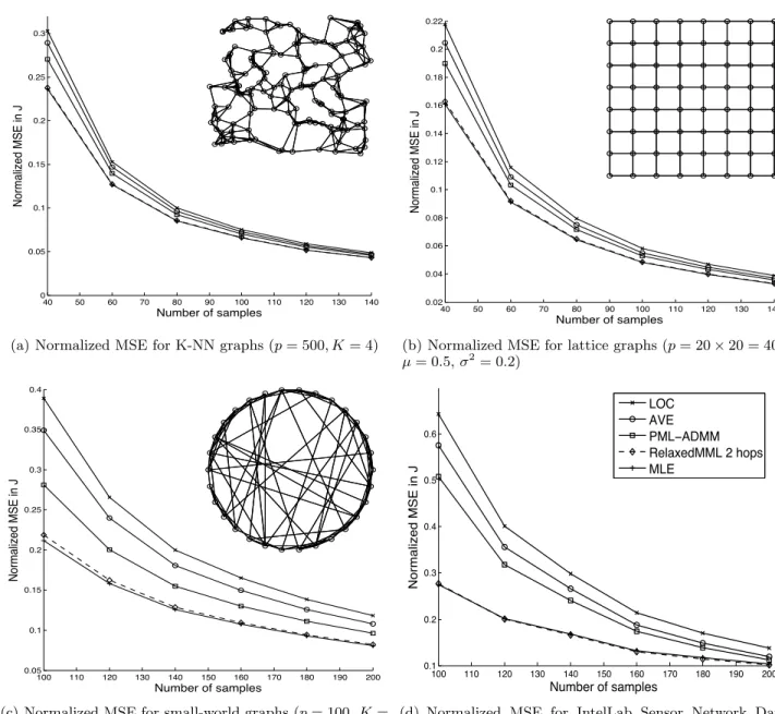
(a) Normalized MSE for K-NN graphs (p= 500, K= 4)
40 50 60 70 80 90 100 110 120 130 140 0.02 0.04 0.06 0.08 0.1 0.12 0.14 0.16 0.18 0.2 0.22 Number of samples Normalized MSE in J
(b) Normalized MSE for lattice graphs (p= 20×20 = 400,
µ= 0.5,σ2= 0.2) 100 110 120 130 140 150 160 170 180 190 200 0.05 0.1 0.15 0.2 0.25 0.3 0.35 0.4 Number of samples Normalized MSE in J
(c) Normalized MSE for small-world graphs (p= 100,K= 20,β= 0.5) 100 110 120 130 140 150 160 170 180 190 200 0.1 0.2 0.3 0.4 0.5 0.6 Number of samples Normalized MSE in J LOC AVE PML−ADMM RelaxedMML 2 hops MLE
(d) Normalized MSE for IntelLab Sensor Network Data set (Guestrin et al., 2004) (p= 50)
Figure 2: Normalized MSE in the concentration matrix estimates for different networks. The legend in Figure 2(d) applies to all plots.
each class we follow similar experiment settings as in Wiesel & Hero (2012). Specifically, we randomly generate 20 topologies and concentration matrices J, and for each J, we perform 10 experiments in which random samples are drawn from the distribution and the concentration matrix is estimated from the sam-ples. The normalized mean squared errors (MSE), defined as kbJ−Jk2F
kJk2
F
, and averaged over all 200 exper-iments, are reported in Figure 2. An illustration of the graph topology is shown in the top-right corner of each plot. In Figure 2(a) and 2(b), the nodes are posi-tioned according to the physical layout of the network, while in Figure 2(c), we show a common rendering for
a small-world graph. The classes of graphs we consider are:
• K-NN graphs(Figure 2(a)): A K-nearest neighbor graph is a straightforward model for real-world net-works whose measurements have correlations that depend on pairwise Euclidean distances,e.g., sensor networks. For these experiments, we randomly gen-eratep= 500 nodes uniformly over the unit square. Each node is then connected to itsK-nearest neigh-bors, where K = 4. The concentration matrix is initialized as Ji,j =±exp(−0.5·di,j) with random sign, where di,j is the distance between theith and
di-agonal to ensure positive definiteness.
• Lattice graphs (Figure 2(b)): A lattice graph is appropriate for networks with regular spatial cor-relations. We generate a square lattice graph with
p = 20×20 = 400 nodes and edge weights gen-erated as Ji.j = min{w,1}, wherew is a normally distributed random variable with mean 0.5 and vari-ance 0.2. A small value is added to the diagonal to ensure positive definiteness.
• Small-world graphs (Figure 2(c)): A small-world graph is a useful model for social networks, where most nodes have few immediate neighbors but can be reached from any other node through a small number of hops. We use the Watts-Strogatz model (Watts & Watts-Strogatz, 1998) to gen-erate random small-world networks, with p= 100,
K(mean degree) = 20, and parameterβ = 0.5. Un-der this particular setting, a large fraction of nodes have large second-hop neighborhoods with dimen-sion close top. In general we expect the second-hop neighborhood to scale linearly with respect top. We choose the edge weights to be uniformly distributed and also add a small diagonal loading.
From the experiment results in Figure 2, we can make the following comments. For the graphs that have rel-atively small two-hop neighborhoods, such as the K-NN graphs and the lattice grids, the proposed two-hop relaxed MML estimator almost coincides with the global MLE and outperforms other distributed estima-tors significantly. On the other hand, for graphs such as the small-world networks, the dimensions of the two-hop neighborhoods grow as fast asp. In this case, a noticeable gap emerges between the global MLE and the two-hop relaxed MML estimator. However, these graphs are known to be harder to learn through dis-tributed algorithms (Liu & Ihler, 2011) and therefore the competing estimators’ performance also degrades. The two-hop relaxed MML estimator still outperforms by a large margin.
Computational complexity. In the relaxed MML approach, each local problem has the same structure as the centralized ML problem for which there are many efficient algorithms. Furthermore, the local problems can all be solved in parallel before the final one-step averaging. In our experiments, we used the graph-ical LASSO with known structure (Friedman et al., 2009) for solving both the centralized ML problem and the local problems in the distributed algorithm. For moderate p (number of variables) as in the examples presented here, the total run time of the distributed algorithm with no parallelization is comparable to the centralized one. As p grows however, we would ex-pect the complexity of the distributed algorithm to
scale at most linearly with p (assuming that the lo-cal neighborhood dimension slo-cales more slowly, such as with K-NN graphs and lattice). The growth is even slower if the algorithm can be parallelized. For the cen-tralized algorithm, the dependence of complexity onp
is expected to be at least linear (the growth is much faster when generic solvers are used), and centralized storage/communication is required.
4.2 Real-world data
Finally we apply the estimators to a real-world data set to evaluate their performance and robustness. The
Lab dataset (Guestrin et al., 2004) contains temper-ature information from a sensor network of 54 nodes deployed in the Intel Berkeley Research lab between February 28 and April 5, 2004. This dataset is known to be very difficult with many missing data, noise and failed sensors. We select 50 sensors with relatively stable and regular measurements. To obtain a target concentration matrix, we use 1800 consecutive sam-ples per sensor, interpolate the missing or failed read-ings and de-trend the data using a local rectangular window of 10 samples. Next, we compute the sample covariance and invert it to obtain a sample concentra-tion matrix. This concentraconcentra-tion matrix is then thresh-olded to yield a ground truth graphical model with a sparsity level of 70% zeros. Using knowledge of the sparsity and sampling from the original 1800 samples, we estimate the concentration matrix using the same estimators as before. As shown in Figure 2(d), the proposed two-hop relaxed MML estimator still gives a very tight approximation to the global MLE and its advantage over other distributed estimators is obvious.
5
Conclusion
We have proposed a distributed MML framework for estimating the concentration matrix of Gaussian graphical models. The proposed method indepen-dently solves convex relaxations of marginal likelihood maximization problems in local neighborhoods. A global estimate is then obtained by combining the lo-cal estimates via a single round of lolo-cal averaging. The proposed estimator is shown to be asymptotically consistent and computationally efficient. Its improved performance relative to existing distributed estimators is illustrated through extensive experiments.
Acknowledgement
This research was supported in part by ARO grant W911NF-11-1-0391 and Israel Science Foundation Grant No. 786/11. The authors would like to thank the anonymous reviewers for their valuable comments.
References
Banerjee, O., El Ghaoui, L., d’Aspremont, A., and Natsoulis, G. Convex optimization techniques for fitting sparse Gaussian graphical models. In ACM International Conference Proceeding Series, volume 148, pp. 89–96. Citeseer, 2006.
Chandrasekaran, V., Parrilo, P.A., and Willsky, A.S. Latent variable graphical model selection via convex optimization. Annals of Statistics, 40(4), 2012. Dahl, J., Vandenberghe, L., and Roychowdhury, V.
Covariance selection for non-chordal graphs via chordal embedding.Optimization Methods and Soft-ware, 23(4):501–520, 2008.
Friedman, J., Hastie, T., and Tibshirani, R. The El-ements of Statistical Learning: Data Mining, Infer-ence, and Prediction. Springer-Verlag New York, 2009.
Friedman, Jerome, Hastie, Trevor, and Tibshirani, Robert. Sparse inverse covariance estimation with the graphical lasso. Biostatistics, 9(3):432–441, 2008.
Guestrin, C., Bodik, P., Thibaux, R., Paskin, M., and Madden, S. Distributed regression: an efficient framework for modeling sensor network data. In
Information Processing in Sensor Networks, 2004. IPSN 2004. Third International Symposium on, pp. 1–10. IEEE, 2004.
Johnson, C.C., Jalali, A., and Ravikumar, P. High-dimensional sparse inverse covariance esti-mation using greedy methods. arXiv preprint arXiv:1112.6411, 2011.
Koller, D. and Friedman, N. Probabilistic graphical models: principles and techniques. MIT press, 2009. Lauritzen, S.L. Graphical models, volume 17. Oxford
University Press, USA, 1996.
Liu, Q. and Ihler, A. Learning scale free networks by reweighted `1 regularization. In Proceedings of the
14th International Conference on Artificial Intelli-gence and Statistics (AISTATS), 2011.
Liu, Qiang and Ihler, Alexander. Distributed pa-rameter estimation via pseudo-likelihood. Inter-national Conference on Machine Learning (ICML), June 2012.
Meng, Z., Wiesel, A., and Hero, A.O. Distributed principal component analysis on networks via di-rected graphical models. In Acoustics, Speech and Signal Processing (ICASSP), 2012 IEEE Interna-tional Conference on, pp. 2877–2880. IEEE, 2012. Ravikumar, P., Wainwright, M.J., Raskutti, G., and
Yu, B. High-dimensional covariance estimation
by minimizing `1-penalized log-determinant
diver-gence. Electronic Journal of Statistics, 5:935–980, 2011.
Rothman, A.J., Bickel, P.J., Levina, E., and Zhu, J. Sparse permutation invariant covariance estimation.
Electronic Journal of Statistics, 2:494–515, 2008. Van der Vaart, A.W. Asymptotic statistics, volume 3.
Cambridge university press, 2000.
Wainwright, M.J. and Jordan, M.I. Graphical mod-els, exponential families, and variational inference.
Foundations and TrendsR in Machine Learning, 1 (1-2):1–305, 2008.
Wainwright, M.J., Jaakkola, T.S., and Willsky, A.S. Tree-reweighted belief propagation algorithms and approximate ML estimation by pseudo-moment matching. In Workshop on Artificial Intelligence and Statistics, volume 21, pp. 97. Society for Arti-ficial Intelligence and Statistics Np, 2003.
Wainwright, M.J., Jaakkola, T.S., and Willsky, A.S. A new class of upper bounds on the log partition function. Information Theory, IEEE Transactions on, 51(7):2313–2335, 2005.
Watts, D. and Strogatz, S. The small world problem.
Collective Dynamics of Small-World Networks, 393: 440–442, 1998.
Wiesel, A. and Hero, A.O. Distributed covariance estimation in Gaussian graphical models. Signal Processing, IEEE Transactions on, 60(1):211–220, 2012.
Wiesel, A., Eldar, Y.C., and Hero, A.O. Covariance es-timation in decomposable Gaussian graphical mod-els. Signal Processing, IEEE Transactions on, 58 (3):1482–1492, 2010.