Dissertations
2015
A new formulation for delayed detached eddy
simulation based on the Smagorinsky LES model
Karthik Rudra Reddy
Iowa State University
Follow this and additional works at:
https://lib.dr.iastate.edu/etd
Part of the
Aerospace Engineering Commons
This Dissertation is brought to you for free and open access by the Iowa State University Capstones, Theses and Dissertations at Iowa State University Digital Repository. It has been accepted for inclusion in Graduate Theses and Dissertations by an authorized administrator of Iowa State University Digital Repository. For more information, please [email protected].
Recommended Citation
Rudra Reddy, Karthik, "A new formulation for delayed detached eddy simulation based on the Smagorinsky LES model" (2015).
Graduate Theses and Dissertations. 14505.
Smagorinsky LES model
by
Karthik Rudra Reddy
A dissertation submitted to the graduate faculty in partial fulfillment of the requirements for the degree of
DOCTOR OF PHILOSOPHY
Major: Aerospace Engineering
Program of Study Committee: Paul Durbin, Major Professor
Alric Rothmayer Anupam Sharma Shankar Subramaniam
James Hill
Iowa State University Ames, Iowa
2015
DEDICATION
To my parents Vijayalakshmi and Rudra Reddy, my sister Gayathri, and my wife Rajalakshmi.
TABLE OF CONTENTS
LIST OF TABLES . . . vi
LIST OF FIGURES . . . vii
ACKNOWLEDGEMENTS . . . x
ABSTRACT . . . xi
CHAPTER 1. INTRODUCTION . . . 1
1.1 Background . . . 1
1.1.1 Motivation for hybrid RANS/LES methods . . . 1
1.1.2 Detached eddy simulation . . . 2
1.2 Governing Equations . . . 11
1.2.1 Conservation equations . . . 11
1.2.2 Turbulence model description . . . 13
1.3 Numerical Modeling . . . 16
1.3.1 Spatial discretization . . . 18
1.3.2 Temporal discretization . . . 21
1.3.3 The pressure equation . . . 22
CHAPTER 2. A DDES MODEL WITH A SMAGORINSKY-TYPE EDDY VISCOSITY FORMULATION AND LOG-LAYER MISMATCH COR-RECTION . . . 26
2.1 Introduction . . . 26
2.2 Model Formulation . . . 28
2.3 Test Cases . . . 34
2.3.2 Flow over backward facing step . . . 38
2.3.3 Flow over 2D periodic hills . . . 42
2.3.4 Flow through an air blast atomizer . . . 44
2.4 Conclusion . . . 49
2.5 Acknowledgements . . . 49
CHAPTER 3. ANℓ2ωFORMULATION OF DELAYED DETACHED EDDY SIMULATION . . . 50
3.1 Introduction . . . 50
3.2 Model Formulation . . . 52
3.3 Test Cases . . . 54
3.3.1 Channel flow . . . 54
3.3.2 Flow over a backward facing step . . . 54
3.3.3 Flow over 2D periodic hills . . . 55
3.3.4 Flow through an air blast atomizer . . . 56
3.4 Implementation of Dynamic Procedure . . . 58
3.4.1 Model formulation . . . 60
3.4.2 Test case - flow through a 3D diffuser . . . 62
3.5 Conclusions . . . 64
3.6 Acknowledgments . . . 65
CHAPTER 4. ON THE DYNAMIC COMPUTATION OF THE MODEL CONSTANT IN DELAYED DETACHED EDDY SIMULATION . . . 66
4.1 Introduction . . . 66
4.2 Model Formulation . . . 68
4.3 Test Cases . . . 74
4.3.1 Channel flow . . . 74
4.3.2 Backward facing step . . . 76
4.3.3 Periodic hills . . . 78
4.3.5 Rotating channel . . . 81
4.3.6 Fundamental aero investigates the hill (FAITH) geometry . . . 84
4.4 Conclusion . . . 87
4.5 Acknowledgements . . . 87
CHAPTER 5. CONCLUSION . . . 88
5.1 Summary of Results . . . 88
5.2 Prospects for Future Work . . . 93
APPENDIX A. DERIVATION OF THE MEAN AND TURBULENT KI-NETIC ENERGY EQUATIONS . . . 95
LIST OF TABLES
Table 2.1 Measured mass flow rates for PIV and CFD simulations. . . 47
Table 3.1 Measured mass flow rates for PIV and CFD simulations. . . 57
Table 4.1 Grid resolution for channel flow cases with different Reynolds numbers . . . 74
LIST OF FIGURES
Figure 1.1 Flow over a circular cylinder using SA-URANS . . . 4
Figure 1.2 Flow over a circular cylinder using SA-DES. . . 4
Figure 1.3 Instantaneous vorticity magnitude using SA-URANS . . . 5
Figure 1.4 Instantaneous vorticity magnitude using SA-DES . . . 6
Figure 1.5 Flow over a delta wing . . . 7
Figure 1.6 U+ vs. y+ from DES of channel flow . . . . 10
Figure 2.1 Distribution ofCf for flat plate . . . 33
Figure 2.2 Comparison of shielding function for different models . . . 34
Figure 2.3 Channel flow: effect ofCDES . . . 35
Figure 2.4 Channel flow: U+ and shear stress profiles. . . . 36
Figure 2.5 Channel flow: U+ profiles at differentRe τ. . . 37
Figure 2.6 Channel flow: vorticity contours alongXZ plane . . . 38
Figure 2.7 Channel flow: u′+ ,v′+ and w′+ profiles . . . 38
Figure 2.8 Comparison of production and dissipation limited DDES . . . 39
Figure 2.9 Backward facing step: contours . . . 39
Figure 2.10 Backward facing step: velocity profiles . . . 40
Figure 2.11 Backward facing step: k−ω SST based DDES . . . 40
Figure 2.12 2D periodic hills: velocity profiles . . . 43
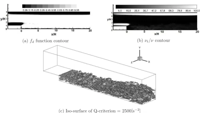
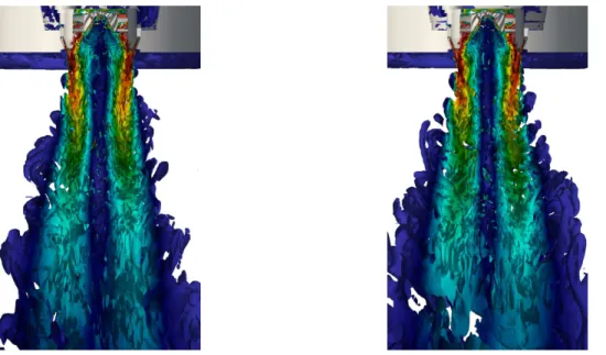
Figure 2.14 Atomizer: contour offd. . . 44
Figure 2.15 Atomizer: iso-surface ofQ. . . 45
Figure 2.16 Atomizer: Qcontours from RANS . . . 46
Figure 2.17 Atomizer: velocity contours along the axial plane . . . 46
Figure 2.18 Atomizer: velocity contours along a radial plane . . . 47
Figure 2.19 Atomizer: velocity profiles along a radial plane . . . 48
Figure 3.1 Channel flow: U+ and shear stress profiles. . . . 54
Figure 3.2 Backward facing step: Iso-surface ofQ. . . 55
Figure 3.3 Backward facing step: Cf distribution . . . 55
Figure 3.4 2D periodic hills: Cf distribution . . . 56
Figure 3.5 Atomizer: Iso-surface of Q . . . 57
Figure 3.6 Atomizer: velocity contours along the axial plane . . . 58
Figure 3.7 Atomizer: velocity contours along a radial plane . . . 58
Figure 3.8 Atomizer: velocity profiles along a radial plane . . . 59
Figure 3.9 Dynamic DDES with no check for mesh quality. . . 61
Figure 3.10 3D diffuser: velocity contours . . . 62
Figure 3.11 3D diffuser: velocity profiles from DDES . . . 63
Figure 3.12 3D diffuser: velocity profiles from dynamic DDES . . . 64
Figure 4.1 Dynamic DDES on a coarse grid . . . 70
Figure 4.2 Dynamic DDES with no check for mesh quality. . . 71
Figure 4.3 Dynamic DDES: limiting function . . . 73
Figure 4.4 Channel flow: U+ profiles at differentReτ. . . 75
Figure 4.6 Backward facing step: dynamic DDES results . . . 77
Figure 4.7 Backward facing step: Climcontours . . . 78
Figure 4.8 2D periodic hills: dynamic DDES results . . . 79
Figure 4.9 3D diffuser: velocity contours . . . 80
Figure 4.10 3D diffuser: velocity profiles from DDES . . . 81
Figure 4.11 3D diffuser: velocity profiles from dynamic DDES . . . 81
Figure 4.12 Rotating channel: velocity profiles at different Ro. . . 82
Figure 4.13 FAITH:Cf contours and velocity profiles. . . 85
Figure 4.14 FAITH: contours of velocity, k,urms andu′v′. . . 85
Figure 4.15 FAITH: contours of km,kr,fdand CDES. . . 86
Figure 5.1 Comparison of production and dissipation limited DDES . . . 89
Figure 5.2 Dynamic DDES with no check for mesh quality. . . 90
Figure 5.3 3D diffuser: velocity profiles from DDES . . . 90
Figure 5.4 3D diffuser: velocity profiles from dynamic DDES . . . 90
Figure 5.5 Channel flow: U+ profiles at differentReτ. . . 91
Figure 5.6 Channel flow: comparison of DDES and dynamic DDES. . . 92
ACKNOWLEDGEMENTS
My heartfelt thanks to Dr. Paul Durbin for guiding me these past three years. His insights and approach to research have been a source of inspiration, and I feel honored to have learnt from him.
I would also like to thank Dr. Alric Rothmayer, Dr. Anupam Sharma, Dr. James Hill and Dr. Shankar Subramaniam for kindly serving on the POS Committee. Special thanks to Dr. Alberto Passalacqua for the discussions I had with him regarding OpenFOAM.
The financial support from NASA Grant NNX12AJ74A and Pratt & Whitney is gratefully acknowledged, without which my PhD dreams would’ve never materialized.
The learning curve I experienced with OpenFOAM would’ve been steeper if it weren’t for Sunil. I’ve had several discussions with him regarding the code, which definitely saved me a lot of time. Special thanks to Elbert and Varun — I learnt a lot from the many technical and not-so-technical discussions we’ve had. I’d also like to thank my colleagues Xuan, Zifei, Rikhi, Farid and Umair, who’ve shared conversations and office space with me over the past three years.
My time in Ames and at Iowa State University has been quite pleasant, thanks to my friends Kannan, Suganthi, Subbu, Avinaash, Monalisa, Bharat and everyone else. I’ve also had many memorable trips with my friends from Georgia Tech — Manu, Aditya, Sangeetha, Ravi, Mahaadevi, Deepa, Vidisha, Ketaki, Apurva, Preethi, Ranjini and so many others — I’ll never forget our time together, and how much fun we had.
Finally, my pillars of support — my family. Words won’t suffice to acknowledge their role. To my parents and sister, for their constant encouragement and motivation which was instrumental in my decision to pursue a PhD, and to my wife, for her support, patience, and faith in me — thank you.
ABSTRACT
This dissertation describes an alternate formulation for Delayed Detached Eddy Simulation or DDES. Detached Eddy Simulation (DES) falls under the category of hybrid RANS/LES mod-els where a single turbulence model functions as either a RANS (Reynolds-Averaged Navier-Stokes) or an LES (Large Eddy Simulation) model. Certain fundamental issues were identified in the original DES formulation, which led to revised formulations such as the Delayed DES (DDES) and Improved DDES (IDDES) with increasing complexity, which negatively impacted the readability of the model.
This is the motivation to explore an alternate formulation for DES which aims to correct the issues found in the original DES, while at the same time being simple and easy to understand. Towards this end, the eddy viscosity formulation in a given RANS model is modified such that it mimics the Smagorinsky LES subgrid viscosity expression when the model is in eddy simulation mode. The resemblance of the resulting DES formulation to the Smagorinsky model allows the implementation of a dynamic procedure to compute the model constant, similar to the dynamic Smagorinsky model. This was found to improve the model performance in several cases. The description of this alternate DES formulation and the implementation of a dynamic procedure in this model will be the major focus of this dissertation.
CHAPTER 1. INTRODUCTION
1.1 Background
1.1.1 Motivation for hybrid RANS/LES methods
Turbulence is commonly encountered in practical fluid flows. It results in much larger skin friction, heat transfer rates and species mixing, compared to laminar flows, which makes accurate prediction of turbulent flows practically important. Hence, turbulence modeling is an inevitable portion of any Computational Fluid Dynamics (CFD) code which hopes to simulate any real-world geometry.
A common view of turbulent flows is that they consist of a range of scales, with the size of the large scales determined by the geometry, and the size of the small scales determined by the fluid viscosity. The broad range of spatial and temporal scales observed in a turbulent flow make it impossible to capture the details of all those scales. Resolving the smallest scales would require very small cell spacing and time steps. This led to the idea of resolving only a certain range of scales, typically the larger ones, while modeling the effect of the smaller scales. Two of the most popular turbulence modeling approaches are Large Eddy Simulation (LES) and Reynolds-Averaged Navier Stokes (RANS) methods.
The LES method models only the smallest scales while resolving all the larger scales. Hence, in general, it is able to produce accurate results for a wide range of flow configurations. However, as the Reynolds numberReof the flow increases, the range of scales to be resolved also increases. This leads to increased computational cost when using LES models for highRe flows, which is usually the case for practical engineering configurations. The computational resources required to simulate such a flow using an LES model are prohibitive (Spalart (2000)).
RANS methods on the other hand capture only the mean flow (or sometimes only the largest scales) while modeling the effect of all the fluctuations. Since a much larger portion of the scales are now being modeled, this leads to a larger error in the computed solution (in general). RANS models are usually calibrated based on attached flows such as flow over a flat plate or channel flow, and hence they work well for such cases. However, for cases involving a separation region, they may be inaccurate (Spalart (2000); Hunt (1990)).
The computational expense of LES and the inaccuracies of RANS for more complex flows motivated the development of hybrid RANS/LES methods. In wall bounded flows, much of the expense of LES arises due to a requirement for small cell spacing in the boundary layer. Hence the idea of using a RANS method to compute the attached boundary layer region and an LES method to compute the flow past the separation point is an attractive proposition cost-wise. Hybrid models are relatively new in the field of turbulence modeling, and have garnered the interest of many researchers.
1.1.2 Detached eddy simulation
Hybrid RANS/LES methods can be broadly classified into 2 categories: zonal and non-zonal. Possibly the most obvious approach of concocting a hybrid model is to take a RANS model, and an LES model, and use them simultaneously in separate, user-defined regions within the flow domain - this is the zonal approach. A concern with such in approach is the interface between the RANS and LES regions, where some kind of interpolation needs to be used in order to provide seamless transition between the 2 regions, and is the focus of several investiga-tions (Schluter et al. (2004); Batten et al. (2004)). Another, more obvious, concern lies in the determination, by the user, of which regions should be simulated with RANS or LES methods. This process is likely to be error-prone and based on a trial-and-error approach, especially for complex geometries.
The non-zonal approach, as the name suggests, is one where the user is not required to specify the RANS and LES regions. One of the most popular non-zonal hybrid RANS/LES
methods is Detached Eddy Simulation (DES), which was first proposed by Spalart et al. (1997). The original DES formulation was based on the Spalart-Allmaras (SA) RANS model (Spalart and Allmaras (1994)) and it introduced a modified length scale definition
˜
d= min(d, CDES∆), (1.1)
where
CDES= 0.65,
∆ =hmax= max(dx, dy, dz).
dis the distance from the wall, ∆ is the maximum cell spacing andCDES is a model constant.
Substituting ˜dfordin the SA-RANS model is the only change required to obtain the SA-DES formulation. In the near-wall region, equation (1.1) yields ˜d = d which makes the DES for-mulation behave like the base SA-RANS model. As we move away from the wall, eventually
˜
d=CDES∆. Using this reduced value for ˜dinstead of denhances the dissipation term in the
effective eddy viscosity equation of the SA-RANS model, leading to a reduction in the eddy viscosity value. This allows the model to sustain/generate fluctuations, thus behaving like an LES model.
Another approach similar to DES is the Scale-Adaptive Simulation (SAS) by Menter and Egorov (2010). SAS also switches between a pure RANS and an LES-like behaviour. Here, the switch is independent of the grid spacing and instead relies on the local flow physics. However, this approach fails to sustain turbulent fluctuations in a channel flow.
A classic example of a case with a large separation region is the flow over a circular cylinder. Indeed, the prediction of such cases with massive separation was one of the main goals of DES. Figure 1.1 shows the vorticity isosurface obtained using the Spalart-Allmaras URANS model. As expected, the 2D URANS fails to predict the three-dimensionality in the solution. The 3D URANS solution is relatively better in this aspect, although the three-dimensionality is still coarse. The same geometry and flow configuration was simulated with the SA-DES model
(a) 2D URANS
(b) 3D URANS
Figure 1.1: Flow over a circular cylinder using the SA-URANS model. Figure reproduced from Spalart (2009).
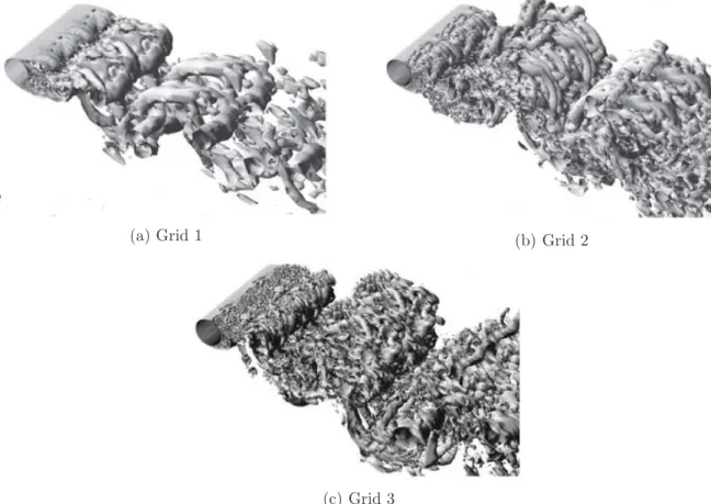
(a) Grid 1 (b) Grid 2
(c) Grid 3
Figure 1.2: Flow over a circular cylinder using the SA-DES model for 3 different grids. Figure reproduced from Spalart (2009).
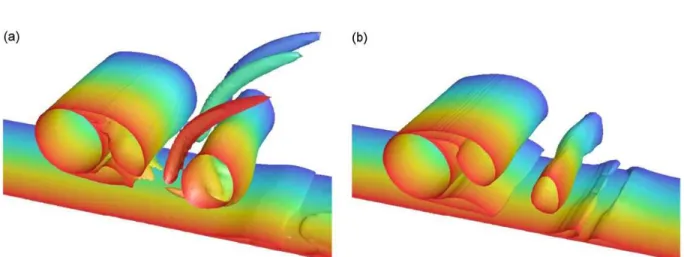
Figure 1.3: Iso-surfaces of the instantaneous vorticity magnitude using SA-URANS. a)H/D= 0.6 b)H/D= 0.2. Reprinted from Nishino et al. (2008) with permission from Elsevier.
using 3 different grids, with the results shown in figure 1.2. Among the 3 grids, grid 1 is the coarsest while grid 3 is the finest. The DES model is able to resolve the three-dimensionality of the flow. As the mesh resolution improves, more and more small scale structures are resolved. Contrary to the behaviour of the DES model, the RANS model did not show any improvement with grid refinement.
Another similar study comparing the behaviour of URANS and DES was carried out by Nishino et al. (2008). Here, the flow over a circular cylinder adjacent to a solid wall was simulated. 2 geometric parameters of importance here are the cylinder diameter D, and the distance between the cylinder and the ground H. Several simulations were carried out using both SA-URANS and SA-DES for different values of the gap ratio H/D. The cessation of vortex shedding occurs when the gap ratioH/D is reduced below a certain threshold value. This had been observed experimentally by Nishino and Roberts (2008). Specifically, the vortex shedding was no longer observed forH/D= 0.2. This behaviour, however, was not observed in the URANS simulation. Figure 1.3 shows vortex shedding occurring even for the H/D = 0.2 case. On the other hand, DES was able to reproduce the correct behaviour. Figure 1.4shows the cessation of vortex shedding for H/D= 0.2.
Figure 1.4: Iso-surfaces of the instantaneous vorticity magnitude using SA-DES. a)H/D= 0.6 b)H/D= 0.2. Reprinted from Nishino et al. (2008) with permission from Elsevier.
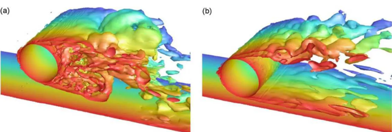
The flow over a delta wing at high angle of attack was studied by Morton (2003) using the SA-DES model. The wing is at an angle of attack α = 27◦
, a flow Mach number M = 0.069 and Reynolds number (based on the chord) Rec = 1.56×10⁶. The simulation was carried out
on 4 different grids. Figure 1.5 shows the vorticity iso-surfaces and the turbulent kinetic energy measured along the core of the vortex. DES is able to capture the unsteadiness well, and the results improve as the mesh is refined, both qualitatively (more small scale structures resolved) and quantitatively (more accurate turbulent kinetic energy prediction).
Besides the cases described thus far, the SA-DES model was shown to produce good results for several different flow configurations such as a landing-gear truck (Hedges et al. (2002)), ground vehicles (Kapadia et al. (2003); Maddox et al. (2004); Roy et al. (2004); Spalart and Squires (2004); Sreenivas et al. (2006)), active flow control by suction/blowing (Spalart et al. (2003); Krishnan et al. (2004)) and aerodynamic noise (Mockett et al. (2008); Greschner et al. (2008)) among others.
Additionally, it was also shown that the DES formulation is not exclusive to the SA-RANS model, but is applicable to other RANS models as well. Strelets (2001) applied the DES formulation to thek−ωSST RANS model of Menter (1993). The wall distancedwas replaced
(a) Instantaneous vorticity iso-surfaces colored by the spanwise component of vorticity a) G1 (1.2M cells), b) G2 (2.7M cells), c) G3 (6.7M cells) d) G4 (10.7M cells)
(b) Normalized resolved turbulent kinetic en-ergy for the four grids
Figure 1.5: Flow over a delta wing at α= 27◦
,M = 0.069 and Rec= 1.56×10⁶. Reproduced
from Morton (2003).
by a RANS length scale ℓk−ω such that
ℓk−ω= √ k β∗ω, β ∗ = 0.09, ˜ ℓ= min(ℓk−ω, CDES∆). ˜
ℓwas used (instead of ˜d) to enhance the dissipation term in thek−ω SST RANS model. The performance of this DES formulation based on the SST RANS model was shown to be similar to the SA-DES model, which demonstrates that the concept of DES is not exclusive to the SA-RANS model.
However, despite the promising performance of DES, a couple of fundamental issues were identified.
The first issue is related to how the DES formulation switches between RANS and LES behaviour. From equation (1.1), we observe that the switch is dependent only on d and ∆, the latter of which is a grid parameter, making the switching criterion entirely dependent on the grid (for stationary meshes). This means that it is possible to generate a grid such that
when the model switches from RANS to LES, the cell spacing is not fine enough to reproduce LES content, leading to an underprediction of the resolved Reynolds stresses. This was termed Modeled Stress Depletion (MSD) by Spalart et al. (2006). In severe cases, this could lead to premature flow separation due to underprediction of the local wall shear stress. This was demonstrated by Menter and Kuntz (2002), who used a DES formulation based on thek−ωSST RANS model (Strelets (2001)), for the case of a flow over an airfoil, where a local near-wall grid refinement led to premature flow separation and was termed Grid-Induced Separation (GIS). The separation here is determined by the grid, rather than the flow physics. Menter and Kuntz (2002) corrected this behaviour by utilizing the blending functions of the k−ω SST model to prevent the DES model from switching to LES behaviour within the boundary layer. A similar, more generic, approach was taken by Spalart et al. (2006) to prevent premature switching of the model behaviour. Rather than using the blending functions of thek−ωSST model (which are exclusive to that model), a more generic “shielding” function fd, was introduced as shown
below: ˜ d=d−fdmax(0, d−CDES∆), (1.2) fd= 1−tanh([8rd]3), (1.3) rd= νT +ν κ2d2pU i,jUi,j , (1.4)
where νT is the eddy viscosity, ν the kinematic viscosity, κ the Von K´arm´an constant, and
Ui,j the velocity gradient tensor. The shielding functionfd is formulated such that within the
boundary layer fd = 0, and outside the boundary layer fd = 1, with fd transitioning from 0
to 1 towards the edge of the boundary layer. Hence ˜d = d within the boundary layer, and the DES model always exhibits RANS behaviour. This prevents MSD from occurring, which also avoids GIS. Outside the boundary layer equation (1.2) yields the original DES behaviour (equation 1.1). This formulation was termed Delayed DES or DDES (Spalart et al. (2006)). Like the DES formulation, DDES is not exclusive to the SA-RANS model, and can be applied to other RANS models as well. This is achieved by rewriting equation (1.2) as
where lRAN S and lLES are the RANS and LES length scales respectively, defined based on
the RANS model used. For the SA-RANS model, lRAN S = d and lLES = CDES∆ yielding
lDDES = ˜d. The generic DDES formulation has been applied to the k−ω SST RANS model
by Gritskevich et al. (2012).
Application of DES to simulate turbulent channel flows led to the exposure of a second issue. Channel flow simulations by Nikitin et al. (2000) and Piomelli et al. (2003) resulted in 2 log-layers in the non-dimensional mean velocity profiles, each corresponding to the RANS and LES regions. Figure 1.6 shows the non-dimensional velocity profiles obtained for several channel flow cases, corresponding to a wide range of Reynolds numbers Reτ (based on the
friction velocity uτ) and grid resolutions. All the profiles show that the log-layer computed by
the LES region is offset from that computed by the RANS region by ≈3U+. This was termed
Log-Layer Mismatch (LLM), and it was observed even in the DDES formulation (Spalart et al. (2006)). This led to another formulation known as Improved DDES or IDDES, by Shur et al. (2008), which aimed to alleviate LLM in addition to MSD. The IDDES formulation is partially reproduced below:
lIDDES = ˜fd(1 +fe)lRAN S+ (1−f˜d)lLES,
lLES =CDES∆, ∆ = min[max(Cwdw, Cwhmax, hwn), hmax],
˜
fd= max[(1−fdt), fB], fdt = 1−tanh[(8rdt)3],
fB = min[2 exp(−9α2),1], α= 0.25−dw/hmax,
fe=fe2max[(fe1−1),0], fe1 = 2 exp (−11.09α2), if α ≥0, 2 exp (−9.0α2), if α <0, fe2 = 1−max(ft, fl), ft= tanh[(c2trdt)3], fl= tanh[(c2lrdl)10], rdt = νT κ2d2 w p Ui,jUi,j , rdl = ν κ2d2 w p Ui,jUi,j .
Figure 1.6: U+vs. y+profiles in channel flow for severalRe
τ values and grids. Velocity profiles
have been shifted by 5U+ units for the sake of clarity. Reprinted with permission from Nikitin
Clearly, the IDDES formulation is more involved than the DDES formulation. Several new functions have been introduced, some of which are empirical in nature. This makes the for-mulation seem ad hoc, and hard to understand. This additional complexity of the IDDES formulation was acknowledged by the original authors (Shur et al. (2008)).
The complexity and empiricism of the IDDES formulation is the motivation to explore an alternate, simpler DES formulation which can overcome both MSD and LLM, and will be the major focus of this dissertation. We expect a DES model to behave like a RANS model in the near-wall region, and switch to eddy simulation behaviour away from the wall. Hence one possible approach to come up with a new DES formulation is to start with a RANS model, and modify its formulation such that it behaves like a known LES model away from the walls. This can be accomplished by modifying the RANS eddy viscosity such that it mimics (for example) the Smagorinsky subgrid viscosity in the eddy simulation region. This approach will be detailed in Chapter 2, following a brief description of the governing equations and numerical modeling in the following sections.
1.2 Governing Equations
1.2.1 Conservation equations
For all cases/simulations considered in this dissertation, an incompressible flow assumption is made. Additionally, the fluid stresses are assumed to be Newtonian, with constant kinematic viscosity ν. With these assumptions, the governing fluid flow equations, in tensor notation, are: ∂Ui ∂xi = 0, (1.6) DUi Dt =− 1 ρ ∂P ∂xi +∂τij ∂xj , (1.7) τij =ν ∂Ui ∂xj +∂Uj ∂xi = 2νSij, (1.8)
whereUi is the velocity vector,ρthe fluid density,P the pressure andSij the strain rate tensor. D
Equations (1.6) and (1.7) are the mass and momentum conservation equations respectively. In the case of a turbulent flow, these equations would represent the action of all fluid scales. However, when using a turbulence model, only a certain range of the larger scales are resolved, with the effect of the smaller scales being modeled. A common approach of separating the resolved and unresolved scales by using a filter is shown below:
Ui=Ui+ui.
Ui represents the filtered (or resolved) portion of the velocity, while ui is the residual (or
unresolved) portion. If the filtering operation is applied to the governing equations, it leads to a set of equations for the filtered variables as shown:
∂Ui ∂xi = 0, (1.9) ∂Ui ∂t + ∂UiUj ∂xj =−1 ρ ∂P ∂xi + ∂ ∂xj [2νSij]. (1.10)
Here, it is assumed that differentiation and filtering commute. Details of the filtering operation can be found in several standard references such as Pope (2000).
In general,UiUj6=UiUj which makes equation (1.10) different from the momentum equation
(1.7). Defining
τijs =UiUj−UiUj,
equation (1.10) can be rewritten as DUi Dt =− 1 ρ ∂P ∂xi + ∂ ∂xj [2νSij]− ∂τs ij ∂xj . (1.11)
The term τijs represents the effect of the unresolved scales on the filtered velocity field. Since only the larger scales are being resolved, the value of τs
ij is not known explicitly and needs to
be modeled. The type of filter used determines the modeling approach (RANS or LES). For RANS models, the filtering operation represents an ensemble average such that
ui= 0,
This is known as Reynolds-averaging. Following this equation (1.11) can be written as DUi Dt =− 1 ρ ∂P ∂xi + ∂ ∂xj [2νSij]− ∂uiuj ∂xj . (1.12)
Equation (1.12) is the governing equation for the average/mean velocity. uiujis known as the
Reynolds stress tensor and needs to be modeled to obtain closure. One of the most common modeling approaches is to express the anisotropic portion of the Reynolds stresses as being proportional to the filtered strain rate tensor, such that
uiuj=
2
3kδij−2νTSij. (1.13) This is popularly known as the Boussinesq approximation. k= 12uiuiis known as the turbulent
kinetic energy. Using equation (1.13), the filtered momentum equation (1.12) now becomes DUi Dt =− 1 ρ ∂ ∂xi (P+2 3ρk) + ∂ ∂xj [2(ν+νT)Sij], ⇒ DUDti =−1 ρ ∂P˜ ∂xi + ∂ ∂xj [2(ν+νT)Sij]. (1.14)
The isotropic portion of the Reynolds stress tensor is absorbed into the pressure to yield a modified mean pressure term ˜P. The effect of the modeled scales is represented by νT, which
acts like the molecular viscosity, and results in a mixing action.
Equations (1.9) and (1.14) are the final forms of the filtered mass and momentum conserva-tion equaconserva-tions which need to be solved. The mass conservaconserva-tion equaconserva-tion is usually not solved explicitly, but is instead satisfied by solving a pressure equation. Details regarding the pressure equation and it’s solution will be presented in section 1.3.
1.2.2 Turbulence model description
The momentum equation (1.14) remains unclosed since νT is yet to be defined. There are
a plethora of methods available to define νT, with each method corresponding to a different
turbulence model. In this dissertation however, we will be focusing on thek−ω RANS model of Wilcox (1993), which is described as:
Dk Dt = 2νT|S| 2 | {z } P −Cµkω+∇ ·[(ν+σkνT)∇k], (1.15) Dω Dt = 2Cω1|S| 2 −Cω2ω2+∇ ·[(ν+σωνT)∇ω], (1.16) νT = k ω, (1.17) where D Dt = ∂ ∂t +Uj ∂ ∂xj , |S|=p2SijSij.
Equation (1.15) describes the evolution of k = 12uiui, which is the turbulent kinetic energy
(TKE). It is possible to formally derive an equation for k by subtracting the mean velocity equation (1.12) from the instantaneous velocity equation (1.7), which would yield a governing equation for the fluctuating velocityui. Multiplying this equation byuiand taking the Reynolds
average of the entire equation then results in the TKE equation (see Appendix A for details). Equation (1.15) is based on this TKE equation.
However, the TKE equation and equation (1.15) are not exactly the same. The mean ve-locity momentum equation has an unclosed Reynolds stress term, which leads to additional unclosed terms in the TKE equation (some of which are of higher order than the Reynolds stress tensor). Some of these terms can be closed by the Boussinesq assumption, while addi-tional approximation would be required to close the remaining terms. The production term in the TKE equation has been closed via the Boussinesq approximation which yields term P. The dissipation and transport terms have been closed using additional approximations, with the final result being equation (1.15).
k= 1
2uiuiis the turbulent kinetic energy. In the RANS formulation, only the mean flow is
resolved, with the effect of all the fluctuations being modeled. Hencekhere is better known as the modeled turbulent kinetic energy.
Broadly, we can think of kas representing the portion of the turbulent kinetic energy due to the unresolved scales. When the DES formulation is introduced into the RANS model, some
of the smaller scales which were previously modeled are now resolved. k would then represent the remaining unresolved scales, and it’s value would change from the RANS value to reflect this.
The second equation (1.16) in the model describes the evolution of ω (∝ kǫ), which is known as the specific dissipation rate and has the units of (time)−1. ǫis the rate of dissipation
of k. Unlike k and the k-equation (1.15), there is no compelling physical meaning behind the definition of ω and the ω-equation (1.16). In 2-equation models, the first variable of choice is almost always k, given that it describes real physical processes. The choice of the second variable/equation however is not as clear. Several models have been proposed which use different variables (besides ω), such as a turbulence length scale ℓ (Rotta (1951, 1968)), a turbulence dissipation time τ (Zeierman and Wolfshtein (1986); Speziale et al. (1990)), the turbulent kinetic energy dissipation rate ǫ (Jones and Launder (1972); Launder and Sharma (1974)) and the enstrophy ζ (Robinson et al. (1995)) whereζ ∼ω2. A discussion/comparison
of the pros and cons of all these different models (not to mention algebraic and one-equation models) is beyond the scope of this dissertation. However, it is worth stating that the k−ω RANS model exhibits very good near-wall behaviour (Wilcox (1993)) compared to other RANS models. In the DES formulation, the RANS model is active only in the near-wall region. Hence it is quite natural to choosek−ω as the base RANS model.
The values of the constants used are
Cµ= 0.09, σk=σω = 0.5, Cω1 = 5/9, Cω2 = 3/40.
These values were determined by calibrating the model to perform adequately for several canon-ical flows such as channel flow, decay of grid turbulence etc.
Solving equations (1.15) and (1.16) to obtainνT would require the specification of boundary
conditions forkandω. Of prime importance are the wall boundary conditions. For a simulation where the wall-normal cell spacing is fine enough such that the viscous sublayer and the buffer layer are resolved, the following boundary conditions are used:
kwall = 0,
ωwall→
6ν
βd2 asd→0.
The specification ofkwallis straight-forward — all velocity values become 0 at the wall and hence
k = 0 at the wall. The ωwall specification however becomes complicated since theoretically,
ωwall =∞due tokwall = 0, and the TKE dissipation (defined by velocity gradients) at the wall
ǫwall6= 0. Thus the wall boundary condition forω instead describes an asymptotic behaviour.
Here β= 0.075 anddis the wall distance at the cell adjacent to the wall.
For simulations where the near-wall region is not well resolved, wall functions would need to be used to mimic the behaviour of the unresolved viscous and buffer layers. Details regarding such wall functions can be found in Esch and Menter (2003). All the simulations presented in this dissertation use fine wall normal cell spacing to resolve the viscous and buffer layers.
Equations (1.15) and (1.16) are now solved to obtain the value of the eddy viscosity νT
from equation (1.17). This is in turn used to attain closure of the filtered momentum equation (1.14). This completes the description of the k−ω RANS model.
The DES formulation described in this dissertation will be based on thek−ωRANS model described thus far, where the eddy viscosity equation (1.17) will be modified and used to limit the production term (with the details presented in Chapter 2).
1.3 Numerical Modeling
To solve the governing equations, the open-source code OpenFOAM (http://www.openfoam.org) was utilized. A description of the basic structure of the code and the algorithms used can be found in Weller et al. (1998). OpenFOAM is an unstructured, Finite Volume (FV) solver, capable of solving an arbitrary number of coupled partial differential equations. A major ad-vantage of using a FV solver is that unstructured meshes can be used easily. This is especially convenient when simulating complex geometries.
In the FV method, the spatial domain is sub-divided into several smaller control volumes (CV). The values of the dependent variables such asUandPare stored at the centroid of each CV in a collocated arrangement. Another option is to store the scalar variables in the cell centroids, while the velocities are stored at the cell faces. This is a staggered arrangement. In OpenFOAM, the collocated arrangement is used.
The governing equations (1.9) and (1.14) expressed in vector form are
∇ ·U= 0, (1.18) ∂U ∂t +∇ ·( ¯UU¯) =− 1 ρ∇P˜+∇ ·((ν+νT)(∇U+∇U T )). (1.19) Uis the filtered velocity vector. In the FV approach, equations (1.18) and (1.19) are integrated
over the CV which yields
Z V (∇ ·U)dV = 0, (1.20) d dt Z V UdV + Z V ∇ · ( ¯UU¯)dV =−1 ρ Z V (∇P˜)dV + Z V ∇ · (νe(∇U+∇U T ))dV , (1.21) where νe=ν+νT is the effective viscosity. The value of the eddy viscosity νT is obtained by
solving thek−ω RANS equations (1.15-1.17). Similar to the momentum equation (1.21), the RANS equations (1.15,1.16) are also solved using the FV approach, with the equations being integrated over a control volume and in time. The discretization of the individual terms in the RANS equations is done in a similar manner as in the momentum equation. Hence only the discretization of the momentum equation will be described in detail, with the same procedure being followed for the RANS equations. The discretization techniques used to approximate these integrals will be explained in section 1.3.1.
In addition to the volume integrals, equation (1.21) also has a time derivative which needs to be solved. This can be solved by employing a temporal discretization, where the solution is marched forward in time, over a time step ∆t, starting from an initial condition. Details regarding the temporal discretization will be presented in section 1.3.2.
1.3.1 Spatial discretization
In the 2nd order FV approach, the values of the variables stored at the centroid of the CV are assumed to be constant over the entire CV. Thus the volume integral within the time derivative becomes
Z
Vc
UdV ≈UcVc, (1.22)
whereVc is the cell volume andUc is the value of the velocity vector stored at its centroid.
In OpenFOAM, some of the volume integrals in equation (1.21) are converted to surface integrals via Gauss’s divergence theorem which states that
Z V ∇ · φdV = I S φ·dS, (1.23)
whereφis an arbitrary tensor field of at least 1st order,S the bounding surface of the volume V, and dS the infinitesimal area vector pointing outward. The surface integrals are in turn approximated as the sum of the fluxes across the cell faces.
I
S
φ·dS ≈X
f
Sf ·φf. (1.24)
The summation here is over all the cell faces. Sf is the face area vector. φf is the value of φ
at the face f and is assumed to be constant over the entire face. Since the variable values are stored at the cell centers, some kind of interpolation needs to be performed to estimate φf.
The requirements of the interpolation scheme to be used varies depending on whether we are using a RANS model or an LES model. An LES model aims to capture small scale fluctua-tions. This means that if the scheme being used is diffusive, it will reduce the amplitude of the fluctuations, and in the worst case, it could completely dampen them. An example of such a dissipative scheme is the Upwind Difference scheme which can be of either first order or second order (Warming and Beam (1976)). Hence although such schemes would be compatible with RANS models, they cannot be used in conjunction with LES or hybrid RANS/LES methods.
Hence it is quite clear that a non-dissipative scheme needs to be used for spatial discretiza-tion. A viable option in this case is the Central Difference (CD) method, which is 2nd order
accurate (Ferziger and Peric (2002)), and assumes linear variation of the solution between 2 control volumes such that,
φf =dφC + (1−d)φN. (1.25)
φC represents the variable value at the current cell, and φN is that at a neighbouring cell for
which f is the common face. d here is a distance factor such that d = |−→f N|/|−−→CN|. |−→f N| is the distance between the centroid of neighbour N and face f. Likewise, |−−→CN| is the distance between the current cellC and neighbourN.
Given that a DES method (which is hybrid RANS/LES) will be used for all the simulations presented in this dissertation, unless otherwise stated explicitly, the Central Difference scheme is the method of choice for the spatial interpolation/discretization of all the terms in the gov-erning equations, in order to minimize errors due to numerical dissipation.
The non-dissipative nature of the CD scheme can be a double-edged sword depending on the application, since it is known to become unstable. A cell Reynolds number Rec can be
defined as
Rec =
U∆ νφ
,
where ∆ is a measure of the cell dimension and νφ is the diffusion coefficient of the variable
φ for which the CD interpolation is being used (νφ = ν for φ =U). For Rec > 2, the CD
method is likely to become unstable (de Villiers (2006)), in which case the mesh would have to be refined to obtain a stable solution.
The convection term in equation (1.21) is simplified using equations (1.23) and (1.24) as follows Z Vc ∇ ·( ¯UU¯)dV = I Sc dS·( ¯UU¯), ≈X f Sf ·( ¯UfU¯f), =X f (Sf ·U¯f) ¯Uf. (1.26)
Here both the flux (Sf·U¯f) and the convected variable ( ¯Uf) are unknown resulting in a quadratic
function for velocity. In order to simplify this, the flux term is computed using velocity values from a previous iteration/time step. Equation (1.26) then becomes
Z Vc ∇ ·( ¯UU¯)dV ≈X f (Sf ·U¯n −1 f ) ¯Ufn. (1.27)
Here the superscriptnrefers to the current iteration for which the variables values need to be computed, while n−1 refers to values from a previous iteration/time step which are known. Typically, the momentum equation is solved iteratively until the velocity values do not change significantly between successive iterations. This ensures that ¯Un−1
f = ¯Ufn towards the end of
the iteration (within a specified tolerance). This will be explained later in section 1.3.3.
Gauss’s theorem is also used to simplify the diffusion term in equation (1.21). This yields, for a generic diffusion term,
Z Vc ∇ ·(νφ∇φ)dV ≈ X f Sf ·(νφ∇φ)f, =X f (νφ)fSf ·(∇φ)f. (1.28)
Equation (1.28) represents the discretization for the diffusion of a generic variable φ. The diffusion coefficient (νφ)f is calculated via the CD method (equation 1.25). The face gradient
(∇φ)f is found using
Sf ·(∇φ)f =|Sf|
φN −φC
|−−→CN| . (1.29) The above equation works only if Sf and −−→CN are parallel, i.e. the mesh is orthogonal. For non-orthogonal meshes, the following relation is used
Sf ·(∇φ)f =|SfCN| φN −φC |−−→CN| | {z } orthogonal +Sfd·(∇fφ)f | {z } non-orthogonal , (1.30) (∇fφ)f =d(∇φ)C + (1−d)(∇φ)N, (1.31) (∇φ)C = 1 Vc X f Sfφf, (1.32)
whereSfCN represents the component ofSf parallel to −−→
CN, andSfd =Sf−SfCN. Equation
(1.31) is analogous to equation (1.25).
Equation (1.30) results in a larger stencil to compute the face gradients when the mesh is non-orthogonal. In order to retain the same stencil as the orthogonal case, the non-orthogonal term is computed explicitly using φvalues from the previous iteration/time step.
The orthogonal correction term could lead to solution instability when the mesh non-orthogonality is high (de Villiers (2006)). Hence the grid used must be constructed such that the non-orthogonality is kept to a minimum.
The discretization described above is applied to the diffusion term in equation (1.21) as follows Z Vc ∇ ·(νe(∇U+∇U T ))dV = Z Vc ∇ ·(νe(∇U))dV + Z Vc ∇ ·(νe(∇U T ))dV , ≈X f (νe)fSf ·(∇U)f +∇ ·[νe∇(U n−1 )T]Vc. (1.33)
In OpenFOAM, the diffusion term is split into 2 terms — one containing∇Uand the other with its transpose∇UT. Treating the transpose term as a diffusion term as well would result in the value of each velocity component become dependent on the other components (since each row in ∇UT contains u,v and w gradients) resulting in a linked system of equations which would increase the computation cost. Therefore, the transpose term is computed explicitly using values from the previous iteration/time step, while the gradient term is treated in a similar manner as the generic diffusion term.
1.3.2 Temporal discretization
The temporal discretization scheme used in OpenFOAM is now described.
In order to obtain 2nd order accurate solutions, both the spatial and temporal discretizations need to be 2nd order accurate. If fn represents the solution at the current time step, then
fn−1, fn+1 are the solutions at the previous and next time step respectively. fn−1 and fn are
approximating the temporal derivative can be obtained using Taylor series expansion forfn−1
and fnaround fn+1 as follows:
fn−1 =fn+1−2ftn+1∆t+ 2fttn+1∆t2+O(∆t3), (1.34) fn=fn+1−ftn+1∆t+ 0.5fttn+1∆t2+O(∆t3), (1.35) ⇒2fn−1 2f n−1= 3 2f n+1 −ftn+1∆t+O(∆t3), (1.36) ⇒ftn+1= 1 ∆t 3 2f n+1 −2fn+1 2f n−1 +O(∆t2). (1.37) The subscripts t and tt represent first and second order differentiation with respect to time. Hence equation (1.37) represents the implicit discretization for the first order time derivative term, which can be used to discretize the temporal derivative in equation (1.21). As can be observed, the discretization is 2nd order accurate in time. Since the spatial discretization is also 2nd order accurate (CD method), the overall accuracy would be of 2nd order.
1.3.3 The pressure equation
The spatial and temporal discretization of all the terms in the integral form of the momen-tum equation (1.21) have been dealt with in sections 1.3.1 and 1.3.2 except for the pressure gradient term.
Thus far we have 2 governing equations (1.20, 1.21) and 2 unknowns - the velocityU and pressure ˜P. However, ˜P only appears in 1 equation. In compressible flows, a state equation relating pressure to density is normally used to compute the pressure. For incompressible flows (as is the case in this dissertation), this is no longer possible and a different equation for pressure is required. The pressure is solved for using the PISO (Pressure Implicit with Splitting of Operators) algorithm of Issa (1986). Once the discretization techniques described in sections1.3.1and 1.3.2are applied to the momentum equation (1.21), a system of equations are obtained
The pressure gradient term ∇P˜ is yet to be discretized. A represents the coefficient matrix obtained after discretization (which is known). The A matrix is now split as
AU=AcU−H, (1.39)
⇒AcU=H− ∇P .˜ (1.40)
Acis the diagonal ofAwhich contains the current cell coefficients. −H contains the off-diagonal
terms which represent the neighbour coefficients multiplied by their respective velocities. Then equation (1.40) can be written as
U= (Ac)−1H−(Ac)−1∇P .˜ (1.41)
Applying mass conservation, we get
∇ ·U=∇ ·[(Ac)−1H−(Ac)−1∇P˜],
⇒ ∇ ·[(Ac)−1∇P˜] =∇ ·[(Ac)−1H]. (1.42)
Since Ac is a diagonal matrix, computing (Ac)−1 is straight-forward. Equation (1.42) is the
Pressure Poisson equation which can be used to solve for pressure. Since mass conservation was employed in the derivation, solving the pressure equation obviates the need to solve the mass conservation equation separately.
Equation (1.42) is written for a single CV as
∇ · " ∇P˜c ac # =∇ · h ac . (1.43)
ac andhare the coefficients for the current cell and its neighbours respectively (hcontains the
velocities as well). Similarly, equation (1.41) is written for a single CV and face values as Uc= h ac − ∇aP˜c c ! , (1.44) (Uc)f = h ac f − ∇P˜c ac ! f . (1.45)
Equation (1.44) is used to compute the velocities at the cell centers once the pressure is known. Likewise, the face values are updated using equation (1.45) to compute the fluxes.
Gauss’s divergence theorem is applied to equation (1.43) which, for a single CV, yields the following X f Sf · 1 ac f (∇P˜c)f = X f Sf · h ac f , (1.46)
where the pressure Laplacian is treated in a similar manner to the generic diffusion term.
The PISO algorithm can now be described:
1. The turbulence variables (k,ω,νT) are first computed using the velocity, pressure and flux
values from the previous iteration/time step or the initial conditions. The individual terms in the turbulence equations are treated in the same manner as those in the momentum equation.
2. The momentum equation is solved using the previous iteration/time step values for ˜P and the fluxes. The matrix system is solved using the Preconditioned BiConjugate Gradient algorithm, with the simplified, diagonal-based, incomplete-LU preconditioner (Ferziger and Peric (2002)). The iterations are repeated until the velocity values between 2 suc-cessive iterations do not differ by a value larger than a specified tolerance. The resulting velocity field is U∗. In general, U∗ does not satisfy the continuity equation since the pressure equation is yet to be solved. This is the predictor step.
3. U∗ is used to update the H matrix and the pressure equation is now solved using the Preconditioned Conjugate Gradient algorithm, with the diagonal incomplete Cholesky preconditioner (Ferziger and Peric (2002)). This is the corrector step.
4. For non-orthogonal meshes, the pressure equation is solved again in order to converge the non-orthogonal component. Depending on the mesh non-orthogonality, 1-2 corrector steps might be required.
5. Once the pressure is known, the velocities at the cell centers and the fluxes at the cell faces are updated using equations (1.44) and (1.45).
6. Steps 3-5 are repeated until the solution variables do not change significantly (based on a user-specified tolerance) between successive iterations.
7. The algorithm now proceeds to the next time step, with the current values used as initial guesses, and the entire solution procedure is repeated. This goes on until either the solution variables do not change significantly between successive time steps, or a certain no: of time steps have passed (depends on user-input).
CHAPTER 2. A DDES MODEL WITH A SMAGORINSKY-TYPE EDDY VISCOSITY FORMULATION AND LOG-LAYER MISMATCH
CORRECTION
K. R. Reddy, J. A. Ryon, P. A. Durbin, (2014)
International Journal of Heat and Fluid Flow, 50, 103-113
The current work develops a variant of delayed detached eddy simulation (DDES) that could be characterized as limiting the production term. Previous formulations have been based on limiting the dissipation rate (Spalart et al. (2006)). A clipped length scale is applied directly to the eddy viscosity, yielding a Smagorinsky-like formulation when the model is on the eddy simulation branch. That clipped eddy viscosity limits the production rate. The length scale is modified in order to account for the log-layer mismatch (a well-known issue with DDES), without using additional blending functions. Another view of our approach is that the subgrid eddy-viscosity is represented by a mixing length formula l2ω; in the eddy field ω acts like a filtered rate of strain. Our model is validated for channel flow as well as separated flows (backward-facing step, 2D periodic hills) and illustrated via an air-blast atomizer.
2.1 Introduction
Hybrid RANS/LES models are considered to have promise for industrial CFD applications, where the idea is to employ RANS in the near wall part of attached boundary layers, and eddy resolving simulation in regions away from the surface. Detached Eddy Simulation (DES) falls under this category of hybrid methods. DES was first proposed by Spalart et al. (1997) and since then, the method has undergone considerable revision. Menter and Kuntz (2002) pointed out that artificial Grid Induced Separation (GIS) could occur if, when the switch from RANS
to Eddy Simulation took place, the reduction of eddy viscosity was not balanced by resolved turbulent content. This effect was termed Modeled Stress Depletion (MSD). Towards this end, the blending functions of the k−ω SST model were used as a “shield” to prevent the model from switching to eddy simulation within the lower part of the boundary layer. Following this, Spalart et al. (2006) introduced a generic shielding function, applicable to any RANS model, and the resulting formulation was termed Delayed DES (DDES) — although it might better be called shielded DES.
Another perspective on DES is that it has an ability to function as a type of Wall-Modeled LES (WMLES). Initial attempts to use the original DES as a WMLES formulation in a channel flow (Nikitin et al. (2000); Piomelli et al. (2003)) resulted in two, mismatched log-layers — one from the RANS branch, and the other from the eddy resolving branch. This anamoly was termed Log-Layer Mismatch (LLM) — an issue which is present in the DDES formulation as well.
Breuer et al. (2003) noted that hmax = max(dx, dy, dz) may not be a suitable length scale to
use in the eddying regions of DES, and that using V1/3 instead, where V is the cell volume,
produced better results. The fact that a different length scale definition is required was also implied in a formulation termed Improved DDES (IDDES) (Shur et al. (2008)), which required the modification of the length scale definition to be used in the eddying region. In addition to revised length scales, more complex blending functions were introduced in order to ensure that the model performed adequately as a WMLES formulation. The blending functions in the IDDES formulation are responsible for allowing the LES functionality within the boundary layer in the presence of turbulent fluctuations, provided the grid is fine enough. And along with a modified length scale definition, they alleviate LLM seen in the channel flow. This is the key difference between DDES and IDDES.
Yet another variation of DES, known as Zonal DES (ZDES) (Deck (2012)) also employs V1/3
(or ∆ω, which depends on the orientation of the vorticity ω as well as the local cell spacing)
in the eddying region. However, as the name would suggest, ZDES requires the user to specify the RANS and eddying regions.
In the present article, a different variant of DDES is developed and applied to the k−ω model (Wilcox (1993)). The motive for the present approach is to make DES more similar to LES in the eddying region. It has been observed (Spalart (2009); Breuer et al. (2003)) that LES often produces more accurate results than DES. Hence, our objective is to make use of DES to reduce near-wall grid requirements (Spalart et al. (2006)) and, simultaneously, to make the eddy viscosity similar to the Smagorinsky formula far from the surface.
Rather than utilizing the length scale in the dissipation term of the k-equation, it is used to define the subgrid eddy viscosity, which is then used to define the production term. This definition of the eddy viscosity makes it a function of the length scale, similar to the definition used for the subgrid eddy viscosity in the Smagorinsky model. This definition additionally pro-vides a method to estimate the value of the model constant by comparing it to the Smagorinsky eddy viscosity formulation. Hence the model can be viewed as a Smagorinsky DES model with k−ω as the underlying RANS model.
Additionally, the length scale is redefined to ameliorate the issue of LLM without requiring the blending functions of IDDES. The absence of any blending functions (as described in Shur et al. (2008)) in the current formulation would indicate that the near wall behaviour of the current model is more similar to DDES than IDDES. This will be dealt with in more detail in
§2.3.1.
The open source code OpenFOAM (Weller et al. (1998)) was used for all the present com-puter simulations. Gaussian finite volume integration with central differencing for interpola-tion, was selected for spatial discretization of equations. Time integration was by the 2nd order, backward difference method. The resulting matrix system was solved using the Pre-conditioned Bi-conjugate gradient algorithm, with the simplified, diagonal-based, incomplete-LU precondi-tioner. Solution for the matrix system at each time step was obtained by solving iteratively, by specifying an appropriate tolerance for the residual norm.
2.2 Model Formulation
The eddy viscosity can be understood as the product of turbulence length-scale times velocity-scale. The DES method is to clip the length scale; but, alternatively, the velocity
scale — or both velocity and length scales — could be clipped. This leads to our proposed method.
Letℓbe a length scale, to be defined. In DES the RANS length scale is clipped by the grid dimension. For k−ω, the RANS length scale is √k/ω and a length scale, ℓ, clipped for DES is defined as (Spalart et al. (1997))
ℓ= minh√k/ω, CDES∆
i
, (2.1)
where CDES is an empirical constant, and ∆ is an appropriate measure of grid size, e.g.,
max[∆x,∆y,∆z]. CDES∆ is a measure of whether the grid can capture the dominant turbulent
eddies. One could alternatively use equation (2.1) to define a clipped velocity uℓ. Multiplying
through by ω, uℓ = min h√ k, ω CDES∆ i . (2.2)
The eddy viscosity k/ω could be represented asℓ2ω or as u2ℓ/ω; they lead to the same result: before clipping, either one isk/ω. After the clip is in effect
νT =ℓ2ω→(CDES∆)2ω, (2.3)
similar to the Smagorinsky model.
The k−ω equations are (Wilcox (1993)) Dk Dt = 2νT|S| 2 −Cµkω+∂j[(ν+σkνT)∂jk], Dω Dt = 2Cω1|S| 2 −Cω2ω2+∂j[(ν+σωνT)∂jω], νT = k ω. (2.4)
The clip (2.2) preempts the first of these; in the eddying region it, rather than thek-equation, defines the velocity scale. If the transport terms were dropped from the second of equations (2.4) it would become ω2 = 2Cω1 Cω2 | S|2 = 400 27 |S| 2.
The standard constants (Wilcox (1993))Cω1 = 5/9, Cω2 = 3/40 were inserted. Then equation
(2.3) becomes νT = (CDES∆)2 20 3√3 p |S|2.
The constant CDES can be estimated by equating this to (Cs∆)2
p
2|S|2, where C
s is the
Smagorinsky constant (≈0.2). This estimate isCDES ≈0.12, which was found to be
satisfac-tory in validation studies (discussed towards the end of the section).
Dropping transport terms from eqn. (2.4) is not legitimate, so one can view the proposed 2-equation DES model as equation (2.4), the clip (2.1or 2.2) and the eddy viscosity definition
νT =ℓ2ω. (2.5)
Away from the wall, theω-transport equation (2.4) is a diffusive smoother of the rate-of-strain field. In that sense, it is a filter of the resolved eddy field. Equation (2.5) is analogous to the Smagorinsky model, in which this ‘filtered’ variable substitutes for the rate of strain. Near the wall, boundary conditions are dominant, and this interpretation of the ω-equation fails; but that is the RANS region.
The DDES modification introduces the shielding function fd(Spalart et al. (2006))
fd= 1−tanh ([Cd1rd]Cd2) [Cd1= 8, Cd2= 3], rd= k/ω+ν κ2d2 w p Ui,jUi,j , (2.6)
into equation (2.1), wherek/ω is the RANS eddy viscosity,ν the molecular viscosity,κthe von K´arm´an constant, dw the distance to the wall, and Ui,j is the velocity gradient tensor.
The DDES length scale is defined as
lDDES =lRAN S−fdmax(0, lRAN S−lLES),
lRAN S = √ k ω , lLES =CDES∆. (2.7)
The length scale lDDES is then used to define the eddy viscosity νT as
νT =lDDES2 ω, (2.8)
so that when fd = 0 the eddy viscosity formula gives νT = k/ω and the model operates in
RANS mode. Alternatively, when fd = 1 and lLES < lRAN S the eddy viscosity formula gives
This definition ofνT is used in the turbulent kinetic energy production term, leaving all the
other terms unaltered. Dk Dt =2νT|S| 2 −Cµkω+∇ ·[(ν+σk(k/ω))∇k], Dω Dt = 2Cω1|S| 2 −Cω2ω2+∇ ·[(ν+σω(k/ω))∇ω]. (2.9)
The standard constants are invoked,
Cµ= 0.09, σk= 0.5, σω = 0.5,
Cω1 = 5/9, Cω2 = 3/40.
By using the same eddy viscosity (equation2.8) in the momentum equation and the production term, the latter retains its usual meaning of energy transfer from the resolved field tok.
So, another interpretation of the present approach is that the production rate is clipped, rather than the original DES approach of clipping the dissipation rate. To highlight this, the k−ω SST based DDES formulation (Gritskevich et al. (2012)) is shown below:
Dk Dt =Pk− √ k3/l DDES+∇ ·[(ν+σkνTRAN S)∇k], (2.10) Dω Dt = αPk νTRAN S −βω2+∇ ·[(ν+σωνTRAN S)∇ω] + 2(1−F1)σω2 ∇k· ∇ω ω , (2.11) where νTRAN S = a1k max(a1ω, F2S) .
The definitions of the several variables involved such asPk,F1 etc can be found in Gritskevich
et al. (2012). We note that the DDES length scalelDDES is used to clip the dissipation term of
thek−equation with the eddy viscosity retaining the RANS definition, whereas in the current approach,lDDES is used to define the eddy viscosity, which in turn clips the production term
of the k−equation.
From a modeling perspective, limiting either the dissipation term or the production term achieves similar objectives. If we consider a flowfield resulting from a RANS simulation, the entire eddy viscosity field would be the modeled effect of all the turbulent scales. DES limits
this modeled component, which allows for unsteadiness to develop as part of the flow solution (either due to a flow instability or due to initial/boundary conditions). This was achieved by enhancing the destruction term of the model equations, based on the DES clip. In the current formulation, this is achieved by limiting the production term instead. A comparison between these two approaches is dealt with in §2.3.1.
In the original DDES formulation
∆ =hmax≡max[∆x,∆y,∆z].
However, based on previous studies (Breuer et al. (2003); Shur et al. (2008); Deck (2012)) it is clear that a different length scale definition needs to be used in the eddying region. We have found that the LLM issue (§2.3.1) is alleviated by redefining ∆ as
∆ =fdV1/3+ (1−fd)hmax, (2.12)
where V is the cell volume. In the eddy simulation region fd = 1 and this gives V1/3 — as
is used in LES. Switching from hmax near the wall to V1/3 farther out reduces ℓDDES and
hence the eddy viscosity. That allows the resolved eddies to develop at small scales. This is the definition of ∆ used for all the cases presented herein.
Rather than equation (2.12), if we simply used
∆ =V1/3, (2.13)
we would still achieve our goal, in the sense that the model will be using V1/3 as the length
scale in the eddying region, for fd = 1. The difference between equations (2.12) and (2.13)
lies in the region where 0 < fd < 1, which lies towards the edge of the boundary layer. In
this region, eqn. (2.12) uses a blend of hmax and V1/3, resulting in a larger value of ∆ than
when using eqn. (2.13), which leads to a larger value forνT. Hence in the absence of turbulent
velocity fluctuations to balance this reduction in the eddy viscosity, eqn. (2.13) would lead to lower νT values, and consequently, lower skin-friction.
A prime example of such a scenario would be the flow over a flat plate. Figure 2.1 shows theCf distribution obtained using both equations (2.12) and (2.13), compared with the RANS
0 2e+06 4e+06 6e+06 8e+06 1e+07 Rex 0 0.002 0.004 0.006 C f k-ω RANS DDES, ∆ = f dV 1/3 + (1 - f d)hmax DDES, ∆ = V1/3
Figure 2.1: Distribution of the skin-friction co-efficient Cf for a flat plate: Solid line - k−ω
RANS (Wilcox (1993)), Dotted line - current DDES with eqn. (2.12), Dashed line - current DDES with eqn. (2.13)
prediction. The mesh used here was constructed such that hmax ≈ δ (δ being the boundary
layer thickness atRex= 107) uptoRex= 5×10⁶, after which the cell spacing was changed such
that hmax ≈ 0.2δ. This corresponds to an “ambiguous” grid spacing (Spalart et al. (2006)),
where MSD (and consequently GIS) could occur. It has been noted (Gritskevich et al. (2012)) that the shielding function fd does not completely eliminate the issue of MSD. This leads to
lower νT and hence, lower Cf. Hence eqn. (2.12) is used for all the cases presented here. To
reiterate, the difference between using equations (2.12) and (2.13) arises only in the absence of turbulent fluctuations. For cases with unsteady flow fields (such as channel flow), they would both yield identical results.
The Cf prediction for the flat plate can be improved by increasing the extent of the shielded
region (Gritskevich et al. (2012)). However tests on a flat plate boundary layer (fig. 2.2) show that values of 8 and 3 for the constants Cd1 andCd2 in equation (2.6) provide adequate
shield-ing, and hence those values were retained.
One final aspect related to the model formulation that needs to be explored is the sensitivity of the model to the value of the model constantCDES. Using the length scale definition (2.12),
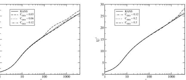
simulations of channel flow were carried out for a range of values of the model constant CDES.
The results are summarized in fig. 2.3. This figure shows limited sensitivity to the exact value of CDES used. Values within 50% of 0.12 produce similar mean velocities. Values as low as
0 0.5 1 1.5 2 y/δ 0 0.2 0.4 0.6 0.8 1 f d SA DDES DDES (SST, 2012), Cd1 = 20 DDES (current), Cd1 = 8
Figure 2.2: Comparison of the fd shielding function for different models: Solid line -
Spalart-Allmaras DDES (Spalart et al. (2006)), Dotted line -k−ω SST based DDES (Gritskevich et al. (2012)), Dashed line - current DDES based onk−ω model (Wilcox (1993))
0.03 and as high as 0.3 produce erroneous mean flow profiles because the RANS-to-eddying switch occurs too near, or too far from the wall.
2.3 Test Cases
2.3.1 Channel flow
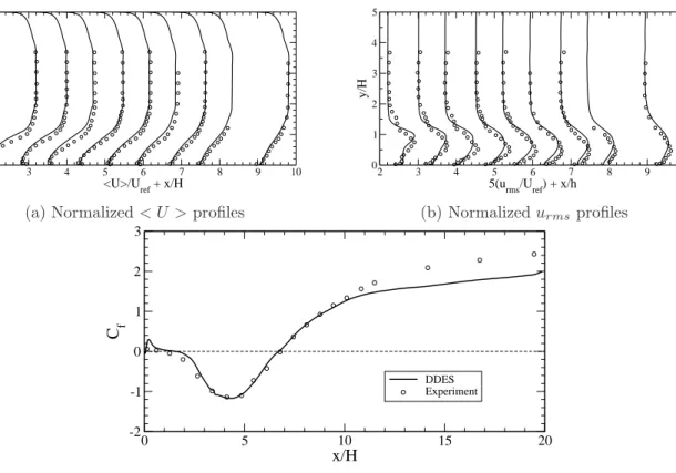
Nikitin et al. (2000) attempted WMLES with the original DES in a channel flow with mixed results. Although it was shown that DES was capable of sustaining LES content, the resulting velocity profile contained two log-layers. Spalart et al. (2006) noted that the DDES formu-lation also exhibits LLM. Not surprisingly, when that same length scale formuformu-lation (except for a changed value of CDES) is adopted for the present model, the same log-layer mismatch
(LLM) is seen, as shown by the dashed line in fig.2.4a; although, the mismatch is not as severe as was observed for other DDES models (Shur et al. (2008)). The solid line in that figure is the mean velocity profile obtained upon using equation (2.12); it is more consistent with the RANS profile. This length scale definition also exhibits better usage of the grid by the LES branch of the model, as shown in fig. 2.4b, where a larger portion of the Reynolds stress has been resolved, compared to the case with ∆ =hmax.
1 10 100 1000 y+ 0 5 10 15 20 25 30 U + RANS C DES = 0.03 C DES = 0.06 CDES = 0.12 1 10 100 1000 y+ 0 5 10 15 20 25 30 U + RANS C DES = 0.12 C DES = 0.2 CDES = 0.3
Figure 2.3: Velocity profiles obtained for differentCDES values in channel flow (Reτ = 4,000)
Further simulations of channel flow at different values of Reτ were done with equation (2.12)
and are shown in fig. 2.5. The velocity profiles are compared to the k−ω RANS model, and the agreement is quite good for all the cases.
In addition to correcting LLM, IDDES differs from DDES in the behaviour of the near-wall regions. Shur et al. (2008) noted that DDES tends to dampen the turbulent content at the RANS-LES interface, which IDDES corrected. In this regard, the current model is more akin to DDES rather than IDDES. Fig. 2.6a represents a wall-parallel plane just before the model switches from the RANS branch to the LES branch and it highlights the dampening effect of DDES at the RANS-LES interface. Fig. 2.6b represents a plane well inside the LES branch, where the turbulent content is better resolved. This region represents a location at which both DDES and IDDES are known to behave similarly (Shur et al. (2008)). The dampening effect of DDES can be seen in the variation of the RMS of velocity fluctuations (fig. 2.7), where the resolved velocity fluctuations obtained with the current DDES model for the case Reτ = 2250 have been compared to DNS data (Hoyas and Jim´enez, (2006)) corresponding to
Reτ = 2003. Overall, the resolved fluctuations are dampened near the RANS-LES interface (at
y/h ≈ 0.1), although the streamwise fluctuations slightly overshoots the DNS values locally. The near-wall peaks are not resolved since the model is in RANS mode, and the major contri-bution to the Reynolds stress would be due to the modeled component (i.e. the eddy viscosity).