VALIDATION OF 3-D ICE ACCRETION DOCUMENTATION AND REPLICATION METHOD INCLUDING PRESSURE-SENSITIVE PAINT
BY
MARIANNE CATHLEEN MONASTERO
THESIS
Submitted in partial fulfillment of the requirements for the degree of Master of Science in Aerospace Engineering
in the Graduate College of the
University of Illinois at Urbana-Champaign, 2013
Urbana, Illinois Advisor:
ii
Abstract
Accurate representation of ice accretions is important to the study and understanding of aircraft icing. For research and certification purposes, replicas of ice accretions generated from icing wind tunnels are fabricated to perform aerodynamic tests in dry-air wind tunnels. The currently employed replication method consists of creating molds from original ice accretions and producing castings from the molds for wind tunnel testing. While this method reproduces the geometric features and aerodynamic effects of the original ice accretions well in the replicated ice shapes, it has several limitations. This method cannot scale the ice shapes to sizes other than the original and does not produce a digital record of the ice shape. Both of these capabilities are desirable in iced-aerodynamics research. To address these needs, NASA developed a methodology to obtain a digital record of ice accretions through the implementation of a laser scanner system. The resulting scan can be used in conjunction with rapid-prototype methods to generate ice shapes for wind tunnel testing. This work is a validation of the 3-D ice accretion measurement methodology where the ice shapes generated by both the currently-used and newly-developed methods from the same initial ice accretion are compared using force balance-derived aerodynamic performance, surface and wake pressures, and pressure-sensitive paint (PSP) data.
The 3-D features of the tested ice shapes necessitated the use of a technique capable of obtaining high resolution data. The PSP technique allowed pressure coefficient data to be obtained over a larger area and at a greater resolution than is possible by only using the surface pressure tap method. The results discussed show the capability of the PSP technique, as implemented in the 3ft by 4ft subsonic wind tunnel at the University of Illinois, to resolve aerodynamic differences between ice shapes made from both the current and newly developed ice accretion replication methods. The same trends were observed in the PSP data as were found in the aerodynamic performance and pressure tap data, and the newly developed 3-D ice accretion measurement methodology produced ice shapes which aerodynamically agreed well with ice shapes generated from the mold and casting method.
iii To my family: Mom, Dad, Allison, and Michelle
iv
Acknowledgements
I would like to thank and acknowledge the many people who supported me throughout my thesis work and graduate studies at the University of Illinois. First, I want to thank my advisor, Professor Michael Bragg, for his guidance and insight, and for enabling me to undertake this project. I want to also acknowledge the FAA and Dr. Jim Riley for their sponsorship of the overall project through Cooperative Agreement Number 10-G-004 of which this research is a part. A thank you is also due to Professor Greg Elliott for answering my questions about pressure-sensitive paint at the onset of the project and for allowing me to borrow much of his optical equipment during testing. Dr. Andy Broeren, Dr. Sam Lee, and Gene Addy from the Icing Branch at NASA Glen Research Center worked closely with me in many aspects of the wind tunnel test and data analysis. They helped me fit my piece of the project into the work as a whole and collaborated with me to acquire the aerodynamic performance data. An immense thank you is due to Greg Milner, Lee Booher, Stephen Mathine, and Dave Foley from the UIUC Aerospace Engineering Research Machine Shop for ensuring that every facet of the mold and casting process went smoothly. They fabricated the components necessary to create the molds and castings and allowed those of us working on the project to invade the shop for most of a semester. Dave especially lent his valued expertise in mold and casting making and in instrumentation of all the many pressure taps.
Jeff Diebold supported much of this work by assisting with model and ice shape installation, modifying the tunnel code to accommodate this specific test, teaching me initially how to run the tunnel, and always being willing to discuss my project and share his aerodynamics knowledge. Thank you also to Dr. Brian Woodard for his tremendous guidance and humor during the writing process and for helping with various aspects of the project. Thank you to Dr. Phil Ansell for sharing his aerodynamics expertise and Brent Pomeroy for giving me access to his library of textbooks and helping me decipher grad school. Thanks also to Ruben Hortensius and Gustavo Fujiwara for being fantastic people
v with whom to share work-space. Thanks for giving our office so much personality and for making my time there both fun and instructive.
I want to recognize some of my incredible friends: Nick Wengrenovich for his many years of friendship and for sharing his positive outlook on life, and Joanie Stupik and Justine Fortier for their never-ending support, encouragement, and laughter throughout our time in graduate school. Thank you from the bottom of my heart for your friendship. Lastly and most importantly, I want to acknowledge my family: my parents, Joan and Nick, and my sisters, Allison and Michelle. Thank you for always being there for me, for supporting me through all that I do, and for being my first and best teachers. Thank you for your love, your understanding, and your belief in me.
vi
Table of Contents
Nomenclature………viii ... 1 Chapter 1 Introduction 1.1 Icing ... 1 1.1.1 Airfoil Icing ... 11.1.2 Swept-Wing Icing and the Need for 3-D Ice Accretion Measurement ... 7
1.1.3 Ice Shape Documentation ... 8
1.2 Pressure-Sensitive Paint ... 11
1.2.1 Pressure-Sensitive Paint Background and Basics ... 12
1.2.2 PSP at Low Speeds ... 16
1.2.3 PSP and Icing Research Background ... 19
1.3 Motivation ... 20
1.4 Objectives and Approach ... 21
... 23
Chapter 2 Experimental Methodology 2.1 Ice Shape Acquisition... 23
2.1.1 NASA Icing Research Tunnel (IRT) Test ... 23
2.1.2 Casting Production ... 24
2.1.3 Rapid-Prototype Shape Production ... 27
2.2 Aerodynamic Testing ... 29
2.2.1 UIUC Aerodynamics Research Lab Wind Tunnel Facility ... 29
2.2.2 Model ... 31
2.2.3 Wind Tunnel Data Acquisition System and Equipment ... 34
2.2.4 Test Procedure ... 44
2.2.5 Wind Tunnel Corrections ... 49
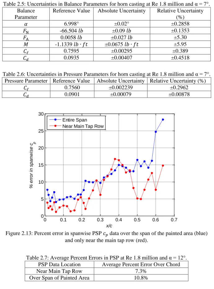
2.2.6 Uncertainty Analysis Results ... 50
... 54
Chapter 3 Results and Discussion 3.1 Clean NACA 23012 ... 55
vii
3.1.1 Aerodynamic Performance ... 55
3.1.2 Validation with Previous Work ... 60
3.1.3 PSP Comparison ... 63
3.2 Horn Ice Shape Comparison ... 74
3.2.1 Geometric Comparison ... 74
3.2.2 Aerodynamic Comparison ... 77
3.2.3 PSP Comparison ... 85
3.3 Roughness Ice Shape Comparison ... 102
3.3.1 Aerodynamic Comparison ... 102
3.3.2 PSP Comparison ... 107
... 123
Chapter 4 Summary, Conclusions, and Recommendations 4.1 Summary ... 123
4.2 Conclusions ... 124
4.3 Recommendations ... 125
References ... 127
... 129
Appendix A Pressure Sensitive Paint Method A.1 Method employed in ARL... 129
... 147
Appendix B Mold and Casting Method ... 160
Appendix C Calculation of Uncertainties C.1 Flow Conditions Uncertainty ... 160
C.2 Force Balance Measurement Uncertainty ... 163
C.3 Pressure System Uncertainty ... 165
C.4 Pressure-Sensitive Paint Uncertainty ... 167
viii
Nomenclature
Cross-sectional area of settling section Cross-sectional area of test section
Axial force coefficient
Drag coefficient Lift coefficient Moment coefficient
Normal force coefficient Axial force acting on model Normal force acting on model
Scaled axial force voltage output from force balance Scaled moment voltage output from force balance Scaled normal force voltage output from force balance
Maximum lift coefficient Lift slope
Minimum drag coefficient
Pressure coefficient
Rate of deactivation due to non-radiative emission
Rate of deactivation due to quenching
Rate of deactivation due to radiative emission
Quarter-chord point offset from balance center in x-direction Quarter-chord point offset from balance center in y-direction
Concentration of quenching particles
‘ Per segment between pressure taps
b Span
C Area of wind tunnel test section h Tunnel height
k/c Horn height non-dimensionalized by chord K1 Constant for wind tunnel corrections
Re Reynolds number
s/c Horn location non-dimensionalized by chord t Airfoil thickness
x Direction parallel to chord
x/c Direction parallel to chord non-dimensionalized by chord y Direction perpendicular to chord
z/b Spanwise direction non-dimensionalized by span Stern-Volmer slope
ix Drag
Intensity of emitted light Lift
Moment Mach number
Static pressure
Specific gas constant for air Planform area Temperature Velocity Uncertainty Chord Dynamic pressure Velocity in pane Greek Symbols Angle of attack
Angle of attack at stall
Velocity increment correction θ Horn angle in relation to chord line
Viscosity coefficient
ν Wavelength
Density
Streamline curvature correction factor Lifetime
Quantum yield of luminescence
Acronyms CAD Computer-aided design
CCD Charge-coupled device
ESP Electronically scanned pressure FAA Federal Aviation Administration FAR FAA Federal Aviation Regulation
IRT NASA Glenn Icing Research Tunnel ISSI Innovative Scientific Solutions, Inc.
NACA National Advisory Committee for Aeronautics NASA National Aeronautics and Space Administration
ONERA Office National d’Etudes et de Recherches Aérospatiales PSP Pressure-sensitive paint
RMS Root mean square RPM Rapid-prototype method
x rpm Revolutions per minute
SLA Stererolithography SLD Supercooled large droplet
TsAGI Central Aero-Hydrodynamic Institute UIUC University of Illinois at Urbana-Champaign
UV Ultra-violet
Subscripts 0 Vacuum or freezing condition ref Reference condition
S Signal luminophore R Reference luminophore ss Settling section ts Test section amb Ambient Freestream
1 Plane downstream of wake
w Wake plane total, o Stagnation sb Solid blockage wb Wake blockage u Uncorrected cor Corrected c/4 Quarter-chord point
1
Chapter 1
Introduction
1.1
Icing
The pursuit of a more complete understanding of aircraft icing is necessary for safe aircraft operation through icing conditions. Studying the process of ice formation on aircraft surfaces and the aerodynamic effects associated with ice accretion enables improved design, enhanced certification procedures, and more accurate computational prediction tools. Much of the past icing research has focused on ice formation and iced-aerodynamics of airfoils. Currently, airfoil icing is reasonably well understood, so the icing research focus is progressing towards improving the understanding of swept-wing icing.1,2 The work reported here is part of the research necessary to build upon the current understanding of airfoil icing in order to study swept-wing icing.
1.1.1
Airfoil Icing
Iced-airfoil aerodynamics can be divided into the four main classifications defined by Bragg et al.3 These classifications, roughness, horn, streamwise, and spanwise-ridge ice, are based on ice-shape geometry and resulting flowfield. A brief description of the definition and aerodynamic penalties of each ice shape type follows.
1.1.1.1 Roughness Ice
Roughness ice is formed during the beginning stages of ice accretion in either glaze or rime conditions, and is characterized by small-scale ice features that do not greatly alter the airfoil contour.3 Roughness ice tends to consist of three zones: a smooth zone, rough zone, and feather region, as were defined by Anderson and Shin.4 Figure 1.1 shows these regions. The smooth zone exists at the airfoil leading edge encompassing the stagnation point. Further downstream is the rough zone on both upper and lower surfaces, followed by
2 the feather region. The roughness features in the rough and feather zones are larger than the boundary layer height for typical flight Reynolds numbers and are the beginnings of significant ice shapes.3 Each isolated roughness element, for low roughness density, acts as a flow obstacle over which the flow separates. This increases skin friction on the surface, which can lead to earlier transition and trailing-edge separation. Roughness ice is associated with increased drag, decreased maximum lift, and lower stall angle of attack. Bragg et al.3 state that the specifics of the roughness’ height, density, and chordwise location determine the extent of the aerodynamic penalties. The location of roughness most detrimental to performance is at the location of minimum pressure where the clean pressure peak occurs. The presence of roughness at this location causes a significant amount of energy to be extracted from the boundary layer, which results in lost lift and increased drag.
Figure 1.1: Typical ice roughness geometry.4 1.1.1.2 Horn Ice
Horn ice is formed during glaze ice conditions, where water droplets do not freeze directly on impact with the surface but flow along the chord for a distance before freezing.5 This behavior yields a buildup of ice slightly downstream from the airfoil leading edge which protrudes into the flow. A simplified horn ice shape can be viewed in Figure 1.2. Horn ice shapes are characterized by their height (k/c), angle to the chord line (θ), and location along the chord (s/c). The aerodynamics of an airfoil with a horn ice shape are dominated by the presence of a separation bubble behind the horn.3 The flow separates off the horn tip due to the severe adverse pressure gradient there and forms a separation bubble similar to the long separation bubbles described by Tani.6 The separated shear layer transitions to turbulent
3 flow at some point after separation. The increased mixing and momentum associated with transition enable the shear layer to reattach to the airfoil surface.3 Upstream of the reattachment line, the flow within the bubble is reversed. The separation bubble has an effect on the airfoil pressure distribution, as seen in Figure 1.3, where the separated flow is indicated by a pressure plateau, followed by region of steep pressure recovery. At higher angles of attack, the pressure decreases at the model trailing edge, which indicates increased pressure drag in comparison to the clean case with no ice accretion. Stall of an airfoil with a horn ice shape has characteristics of thin-airfoil stall.5 Anderson7 describes thin-airfoil stall as occurring as the growth of a separation bubble over the chord to the trailing edge with angle of attack increases, at which point the flow separates and the airfoil stalls.
Variations in flow behavior along the span of an airfoil with a three-dimensional horn shape or two-dimensional horn shape with added roughness, produce cellular-type structures that are evident in surface oil flow visualization. Bragg et al.3 describe how these cells do not seem to correlate to the geometric features of the ice shape. Jacobs and Bragg8 discuss how these features are due to a spanwise instability that produces spanwise vortices and are the result of roughness features on the horn ice shape. Figure 1.4 shows the surface oil flow visualization results from a test by Jacobs and Bragg,8 where spanwise cells are visible behind a two-dimensional ice shape with added roughness. The cells do not exist for cases without roughness.
Overall, Bragg et al.3 summarize that the gross shape (height (k/c), angle (θ), and location (s/c)) of the horn ice shape, not the roughness details, determines the aerodynamic effect. Horn ice shapes cause the most severe aerodynamic penalties.5 They reduce the maximum lift and the stall angle of attack and increase drag due to the flowfield changes from the separation bubble. Additionally, since the horn tip sets the separation point, the aerodynamics of a horn ice shape are effectively independent of Reynolds number.5
4 Figure 1.2: Horn ice shape geometry, adapted from Bragg et al.3
Figure 1.3: Surface pressure distribution for a simulated horn ice shape compared to the clean pressure distribution.3
5
a) b)
Figure 1.4: Surface oil flow visualization comparison between a) 2-D ice shape and b) 2-D ice shape with added roughness.8
1.1.1.3 Streamwise Ice
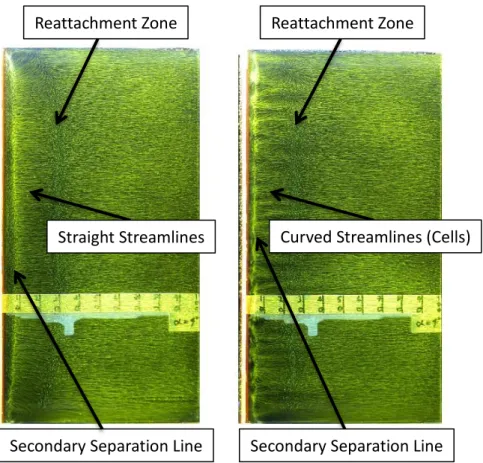
Bragg et al.3 define streamwise ice as ice that forms during rime conditions and generally follows the airfoil contour. Rime conditions occur at temperatures where the impinging water droplets freeze on the surface at impact. The aerodynamic effects of streamwise ice shapes are generally not as drastic as those from horn shapes. Typically, streamwise ice extends forward of the leading edge, sometimes forming a horn-like extension into the flow. Figure 1.5 shows the geometry of a representative streamwise shape. The streamwise-ice flowfield is distinguished from that of the horn by a smaller separation region with a varying separation point. The flow over the airfoil remains attached until near the ice/airfoil junction, where an adverse pressure gradient causes separation. Since the separation region is small, the aerodynamic effects of the bubble are not as severe as those from a horn ice shape separation bubble. This means the roughness of the ice shape has more of an effect, leading to trailing-edge separation having a greater aerodynamic impact.3
Reattachment Zone
Straight Streamlines
Secondary Separation Line Secondary Separation Line Reattachment Zone
6 Figure 1.5: Streamwise ice geometry.9
1.1.1.4 Spanwise-Ridge Ice
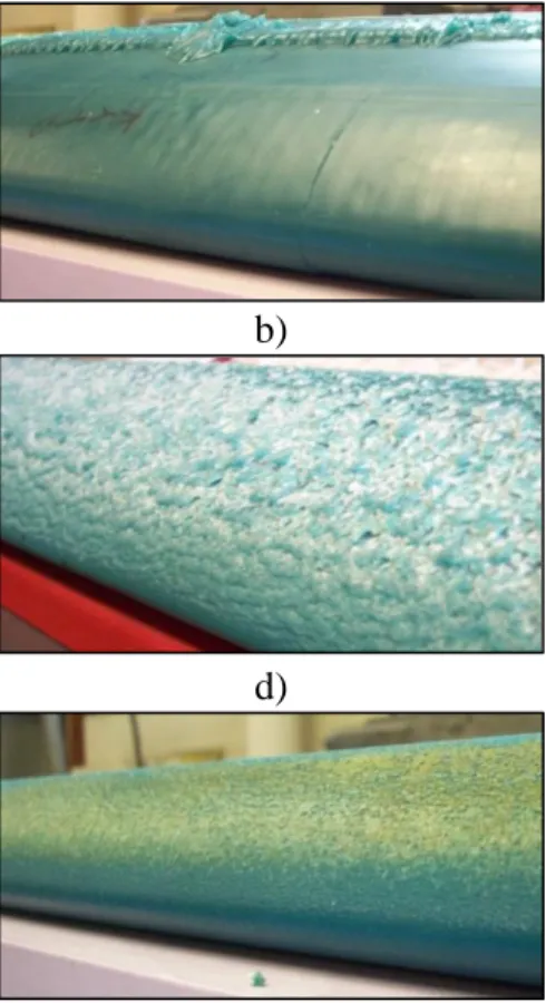
Spanwise-ridge ice forms further downstream from the leading edge and is often the result of a heating device that is not operating at 100% evaporating efficiency. This type of ice shape may also form if the incoming droplet diameters have a large enough momentum to reach the surface behind a leading-edge ice protection system.10 Conditions where these larger droplets, or supercooled large droplets (SLD), form are dangerous since ice protection systems are not as effective. For smaller droplet sizes, once the water passes a heating device operating below 100% evaporating efficiency, freezing can occur behind the de-icer, resulting in a spanwise-ridge ice accretion. Similar to the separation bubble that forms from a horn ice shape, a separation bubble will form from the spanwise-ridge shape and will dominate the flow behavior.3 Bragg et al.3 describe how the spanwise-ridge ice acts as a flow obstacle to the flow on the airfoil. By the time the flow reaches the ridge, the boundary layer is usually turbulent. The flow separates ahead of the ridge, due to the adverse pressure gradient, and forms a bubble upstream of the ice. The flow also separates off of the ridge tip, forming a second separation bubble downstream of the ice. These two bubbles greatly affect the aerodynamics of the flow over the airfoil. The aerodynamics of a spanwise-ridge shape are especially sensitive to ridge height, location, geometric shape, and spanwise variation.3 Figure 1.6 shows a representative geometry of a spanwise-ridge ice shape formed behind a leading-edge ice protection system. Figure 1.6a is a photograph taken upstream of the model looking towards the leading edge and Figure 1.6b is a trace of the same shape.
7
a) b)
Figure 1.6: Spanwise ridge ice shape example, a) photograph and b) tracing, adapted from Broeren et al.11
1.1.2
Swept-Wing Icing and the Need for 3-D Ice Accretion Measurement
To date, a number of swept-wing research programs have studied swept-wing icing. Broeren et al.1 describe past and present work. Most previous work has focused on understanding icing physics, developing computational tools, and testing at low Reynolds numbers on small-scale models. Broeren et al.1 explain the need for further swept-wing icing study and summarize the joint research collaboration between NASA (National Aeronautics and Space Administration), FAA (Federal Aviation Administration), ONERA (Office National d’Etudes et de Recherches Aérospatiales), UIUC (University of Illinois at Urbana-Champaign), and Boeing to accomplish this. The overall goal of this swept-wing icing research program is to develop experimental and computational swept-wing ice simulation methods, and to further understand swept-wing ice formation and aerodynamics. The work described here is a part of one of the phases of this swept-wing icing research program.An essential capability is the ability to accurately record swept-wing ice accretions. NASA previously developed three main processes for recording ice shapes: two-dimensional cross-sectional traces, qualitative photographs, and molds and castings. The trace method yields good information about the general shape of a two-dimensional ice accretion but has large uncertainties based partly on the particular tracing method employed by the person performing the trace. A full three-dimensional understanding is impossible to obtain from traces. Qualitative photographs yield much less information than the traces, yet do provide
8 some three-dimensional knowledge. The mold and casting method is another technique often used by NASA to record ice shapes, and is capable of recording three-dimensional features along a model span. It involves making a mold of an accreted ice shape, and then creating castings from a master mold. The castings can be tested in a dry-air wind tunnel. While the mold and casting method can record three-dimensional features, it is expensive in both materials and time and does not produce a digital record of the ice shape. Therefore, NASA worked to develop a new method of recording ice shapes that could record complex shapes, document shapes digitally, and enable fabrication of shapes for testing. The present work is a part of the validation of the new technique developed by NASA in comparison to the currently accepted mold and casting method.
Once the validation of the new method is complete, the developed process will be used in further phases of the swept-wing icing project. Ultimately this involves the testing of artificially iced models in the ONERA F1 pressurized tunnel. The ice shapes used in this future test will be generated in the NASA Glenn Research Center Icing Research Tunnel (IRT) and recorded using the developed method. Both the replicas of those ice shapes and simulated shapes will be tested in order to determine the degree to which swept-wing ice shapes must be replicated in order to obtain comparable aerodynamic penalties. Ice shape simulations are simplified shapes based on the geometry of initial ice accretions, whereas ice shape replicas possess the three-dimensionality and small-scale features of the original ice accretion. Examples of simulations are two-dimensional extrusions of the ice shape geometry or the representation of a horn by a simple rectangle. Both the mold and casting and 3-D laser scanner and rapid-prototype techniques produce ice shape replicas. In addition to providing results concerning necessary simulation fidelity for swept-wing ice shape testing, the experimental data that will result from the future F1 tunnel test will also provide validations for three-dimensional icing codes. This will aid in the improvement of certification procedures to more accurately, efficiently, and safely certify aircraft for flight in icing conditions.
1.1.3
Ice Shape Documentation
Ice shape documentation is important for the experimental study of icing. Busch5 discusses how icing tunnels are not ideal for aerodynamic testing due to their high turbulence
9 levels, making it necessary for experiments to be performed in other, dry-air wind tunnels. This necessitates the use of ice-shape representations that accurately replicate the flowfield effects and aerodynamics of the original ice accretions. Therefore, methods of recording and simulating the original ice accretions must be used to obtain these representations for use in dry-air wind tunnels. The method that has been used extensively by NASA Glenn Research Center in the Icing Research Tunnel (IRT) is the mold and casting method, mentioned briefly above. This is currently the highest fidelity method of recording ice shapes. With the focus now on swept-wing icing, a more complete documentation of ice shapes is needed. For this reason, NASA developed a 3-D ice accretion measurement methodology to replace the mold and casting technique.28
The other widely used means of documenting ice shapes is through 2-D traces. An ice tracing is obtained by hand tracing an ice accretion in the IRT at a spanwise location. An “ice knife,” or heated metal sheet with the model leading-edge contour cut out from one side, is used to melt the ice at the spanwise location where the trace will be drawn. Once the ice is melted, a cardboard template with the model leading-edge contour cut out from one side is placed in the slot where the ice knife melted the ice. A pencil is then used to carefully draw the two-dimensional geometry of the ice on the cardboard template. This method has been used extensively to understand icing and to provide geometries for computational work.
Ice shape simulation uses simplified geometries based on the original ice accretions to attempt to reproduce the aerodynamics, with varying degrees of fidelity. The simplest simulation is through geometric representation. Mimicking a horn ice shape with a rectangular extrusion of a height, angle, and location similar to the original accretion, or representing a spanwise-ridge shape with a flow obstacle such as a quarter-round geometry, are examples of simplified geometric representation. Two-dimensional extrusions of an ice tracing have a higher fidelity, but do not replicate any three-dimensional effects. Adding distributed roughness elements to these representations helps retain some three-dimensional and roughness effects. Busch5 discusses the specific simulation schemes most applicable to each ice shape classification and analyzes the aerodynamic differences between simulations and castings.
10 1.1.3.1 Current Method: Mold and Casting
In the 1980s, Reehorst and Richter12 developed the mold and casting method as it is currently employed. This method replaced an older method that used wax and plaster and supplemented the two-dimensional ice tracings described previously. The mold and casting method employs molds made from ice accretions in an icing wind tunnel to make castings to be used in aerodynamic dry-air wind tunnel tests. The benefit of this method is its ability to capture three-dimensional features and small roughness details that are unable to be documented by the other previously available methods. The mold and casting process is time consuming due to curing and casting preparation time. Each mold or casting needs from a few hours to overnight to cure. Due to the freezing temperatures required during mold curing to prevent the ice accretion from melting, the specific mold material capable of curing at those temperatures is extremely stiff. Because of this, the mold is destroyed after one casting is made, and another more flexible and durable mold must be made. This adds another step to the process. Each casting must then be cut to size and is usually instrumented with pressure taps in order to be used in dry-air wind tunnel testing. Additionally, the larger the model, the greater the amount of costly molding and casting material is required. The greatest drawback is that these molds and castings are the only documentation of the ice shapes. Possessing a digital copy of the ice shape would be beneficial for record-keeping, comparison, scaling, computation, cost, and ease-of-use purposes.
1.1.3.2 New Method: 3-D laser scanner and rapid-prototyping methods
In response to the need for a more capable and robust ice accretion recording and measurement process, NASA investigated using a 3-D laser scanning system and rapid-prototype methods to record ice accretions and to generate ice shapes for testing.28 Lee et al.28 describe the development process of this system in detail. A 3-D laser scanner is used to scan an ice accretion. The chosen scanner, the Romer Absolute system, is arm-based and proved to be the most effective at scanning shapes, ease-of-use, and operating in the cold temperatures of the IRT. The scanner is used in conjunction with software that is able to fill in holes and gaps in the data to create “water-tight” surfaces, which are completely enclosed, in order to put the data in a form that can be used by rapid-prototype methods.1 The holes for the pressure taps can be added in the software, and are created during the rapid-prototype
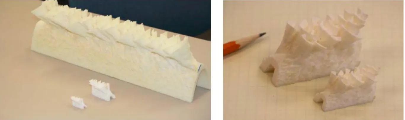
11 process. Initial testing with this process resulted in the ability to scale an ice shape scan to a smaller size and produce small-scale rapid-prototype shapes.28 Qualitatively, Lee et al.28 show the good agreement between full, 1/3, and 1/5 scale shapes. This agreement can be seen in Figure 1.7, where the smaller scale shapes visually to a good job of replicating the features on the full scale shape. Broeren et al.1 include trace data from the castings and scan data at the same spanwise location. They conclude there seems to be good agreement between the methods.
Figure 1.7: Full, 1/3, and 1/5 scale ice shapes made from the 3-D laser scanner method.28
1.2
Pressure-Sensitive Paint
The pressure-sensitive paint (PSP) method is a technique that was first developed in the 1980s and is becoming an accepted method for wind tunnel testing. It is based on photophysical properties that relate emitted intensity from excited paint particles to pressure. A PSP that is applied to an aerodynamic surface can yield pressure data over the entire painted area. This is a great increase in resolution compared to the amount of data that can be measured using discrete pressure taps. The highly three-dimensional flow of a swept wing cannot be well documented using a reasonable number of taps. For this reason, PSP was investigated as a means of obtaining three-dimensional pressure data over the model surface. A first step in this process was to use this method on the airfoil model to see if the PSP could resolve differences between the shapes made from the old and new methods. The effects of the three-dimensional features of the ice on the flowfield could be investigated using PSP.
12
1.2.1
Pressure-Sensitive Paint Background and Basics
1.2.1.1 Basic Theory
The pressure sensitive paint (PSP) technique uses the photophysical processes associated with excited electrons returning to their ground states in order to relate the intensity of luminescing particles, or luminophores, to pressure. Luminescent materials are defined as being “capable of absorbing energy and reemitting visible light.”13
PSP consists of two main components: the luminescing luminophores and the binder in which those luminophores are suspended.
When luminescing particles in PSP are excited using a high-energy excitation source, such as a lamp or laser, the particles absorb the radiative energy from the photon so that the electrons in the paint transition to higher energy levels. In order for these electrons to return to the ground state, the particles must lose the energy they gained through excitation. There are multiple ways this energy can be released, though the two most pertinent to PSP are fluorescence and external conversion through oxygen quenching. Fluorescence is a loss of energy through the emission of photons, and is a specific type of luminescence. Another type of luminescence is phosphorescence, which occurs over a longer time period and involves energy conversions from different energy levels than fluorescence. External conversion is the loss of energy through electron encounters with environmental entities. Oxygen quenching, or the external conversion of excited electrons due to collisions with oxygen molecules, is a competing process to fluorescence in PSP. In order to return to a ground state, the excited particle must lose a specific amount of energy. The greater amount of this energy lost to oxygen collisions in oxygen quenching, the smaller the amount of energy given off through fluorescence and vice versa. In other words, the greater the number of oxygen molecules able to interact with the excited particles, the fewer the photons given off as fluorescence. Since the number of oxygen molecules present is directly proportional to static pressure, the intensity of light emitted by fluorescing particles can also be related to pressure. These reactions form the basis for PSP.
A relationship between the local intensity of the emitted protons from PSP and the local pressure is derived from the Stern-Volmer equation. The Stern-Volmer equation, Eq. 1.1, states the intensity changes between systems with and without a quenching molecule.
13
(1.1)
Φ is the quantum yield of luminescence and is equal to the rate of luminescence over the rate of excitation. I is the intensity of the emitted light. The three temperature-dependent constants, kq, kr, and knr are the rates associated with deactivation due to quenching (kq),
radiative emission (kr), and non-radiative deactivation (knr). [Q] is the concentration of the
quenching molecules. The subscript 0 denotes the non-quenching reference state where no quenching molecules are present. According to Henry’s Law, the partial pressure of oxygen is proportional to the concentration of oxygen. Therefore, [Q] is proportional to the pressure, p. In most aerodynamic applications, it is not feasible to reach a state where no oxygen is present. Therefore, a different reference condition is used. The ratio of the Stern-Volmer equation at this reference state to the state of interest is the form of the equation used in aerodynamic testing. The reference condition is the “wind-off” condition where the wind tunnel velocity is zero. This is in comparison to the “wind-on” condition when the wind tunnel is running at some speed. The pressures over a model in the “wind-on” condition can be determined through the Stern-Volmer equation and known pressures at the “wind-off” condition with Eq. 1.2.
( ) ( )
(1.2)
The coefficients A and B are both temperature dependent since they consist of the k terms, all of which depend on temperature. A more detailed derivation can be found in Liu and Sullivan.14
1.2.1.2 History
The development of pressure-sensitive paint (PSP) technology for aerodynamic applications began in the 1980s in the United States at the University of Washington and independently in the Soviet Union at the Central Aero-Hydrodynamic Institute (TsAGI). However, the effect of oxygen quenching on luminescence has been known since 1935 with the work done by H. Kautsky and H. Hirsch.15 It was not until 1980 that oxygen quenching and fluorescence were used for flow visualization by Peterson and Fitzgerald.16 Following this, luminescent coatings were used in biomedical and chemical applications before being used for aerodynamic testing.14 Since then, a substantial amount of research has been done
14 and progress made in the pressure-sensitive paint area. Once the concept of PSP was proven, most of the research has involved improving the accuracy of the method. Important areas are in temperature effect compensation, image registration, image resection, and increased paint response. A number of methods have been developed to address these concerns and will be described briefly in the next section. Currently PSP is well beyond the proof of concept stage and has begun to be used as an integral flow diagnostic in aerodynamic testing.
1.2.1.3 PSP Methods
There are two main PSP methods: intensity-based and lifetime-based. Intensity-based, or radiometric, PSP uses imaged intensity values to determine surface pressures. Lifetime methods use the decay of luminescent intensity to determine pressure.
The single channel radiometric PSP method is straightforward. Much of the initial PSP research and proof-of-concept was performed with this technique. The “single channel” refers to the sole type of luminophore particles embedded in the paint binder. This is in contrast to other paints that contain multiple fluorescing particles. The single channel method employs the Stern-Volmer relation (Eq. 1.2) as its scientific basis. Two sets of images are used in this method: the wind-off and wind-on intensity images. Since the pressure at the reference wind-off condition is known, the wind-on static pressure over the surface can be calculated. The ratio between the wind-off and wind-on images theoretically removes luminophore concentration, paint thickness, and illumination spatial variation effects. It cannot, however, account for any temperature changes during data acquisition or spatially across the model. Temperature affects the emitted intensity of the paint similarly to how absolute pressure affects the emitted intensity.
Pressure sensitive paints containing multiple luminophores aim to remove the temperature dependence of the paints. A binary paint contains two luminophores: the first, the signal probe, is sensitive to both pressure and temperature, and the second, the reference probe, is only sensitive to temperature. If the temperature dependence of both luminophores is the same, then a ratio of the intensity from the signal probe to the intensity of the reference probe during the wind-on condition will remove the temperature dependence. A paint that is independent of temperature effects is called an ideal paint.17 While the ratio of the signal-probe intensity to the reference-signal-probe intensity theoretically removes temperature
15 dependence, it does not remove luminophore concentration effects. Therefore, wind-off signal and reference images must also be acquired. Paint thickness and illumination effects are removed in the ratio of the signal to reference intensities. To apply this binary PSP concept, a ratio of the ratios is taken. This ratio of ratios is expressed in Eq. 1.3. Binary paints are designed to behave as close to an ideal paint as possible. Of course, the temperature dependence of the two luminophores is not exactly the same, so binary paints are not perfectly ideal. Further research is being performed to minimize temperature effects.
⁄
⁄ ( ) ( ) (1.3)
Theoretically, lifetime PSP methods are not limited by some of the drawbacks from which intensity (radiometric) methods suffer. The lifetime of the paint luminophores’ luminescence is not a function of paint thickness, luminophore concentration, or illumination intensity. This comes with the additional benefit of not requiring a wind-off image, in comparison to most radiometric methods. However, lifetime PSP results are still susceptible to temperature effects, especially at lower speeds and dynamic pressures where the signal to noise ratio is small. At higher speeds and dynamic pressures, the increased signal from the paint is significantly greater than the noise due to temperature. The benefits of the lifetime PSP method are best applied at higher speeds and dynamic pressures.
Lifetime, τ, is defined as the time it takes the emitted intensity from the paint luminophores to decrease by a factor of e when the decay signal can be fit with an exponential function. This method uses intensity images taken from multiple “gates,” or time intervals, in the emission signal during and after an excitation pulse. Figure 1.8 shows typical excitation and emission signals over time with two gates specified.18 During gate 1 in this figure, the camera acquires the first image, which encompasses the time before the excitation pulse until the beginning of signal decay. During gate 2, the camera acquires the second, which encompasses the end of the signal decay. Using the Stern-Volmer equation, the ratio of the integrated intensity over each of the gates can be used to determine a calibration between this ratio and pressure. Temperature effects can be accounted for using a method similar to the binary radiometric method, where a reference probe is used to remove the temperature dependency of the paint.19
16 The main benefit of using a lifetime method, especially at low speeds, is its independence from illumination effects that are the result of model deformation within the intensity field of the excitation source. However, some work has shown that the lifetime method is still susceptible to large amounts of noise that can be removed through a ratio with the wind-off condition, making the lifetime method no more beneficial than the intensity methods.18 Crafton et al.19 explain the noise inherent in lifetime PSP is a result of incomplete chemical processes that leave two types of fluorescing molecules in the paint. Since the lifetimes of these two probes are different and the probes are not distributed evenly within the binder, noise is present in the data.19 Calculating the ratio of the wind-on lifetime with the wind-off lifetime would remove the dependence on the probe concentration, though this removes the main benefit of the lifetime method. In conclusion, Crafton et al.19 recommend carefully implemented binary PSP methods for testing at low speeds. Higher-velocity flows yield higher signal-to-noise ratios, and can therefore benefit from lifetime PSP techniques.
Figure 1.8: PSP excitation and emission decay with two gates for lifetime PSP method.20
1.2.2
PSP at Low Speeds
The difficulties of using the PSP method at speeds in the low-subsonic range stem from smaller pressure variations from the reference condition than are seen at high-subsonic or supersonic speeds. These small variations in pressure yield small variations in intensity and small signal-to-noise ratios.21 For this reason, PSP experiments at low speeds are susceptible to errors that further decrease the signal-to-noise ratio. While these same errors may exist in high-speed PSP data, the associated noise is much smaller than the signal.22
17 Bell21 lists that the major errors in low-speed PSP are random error from photon shot noise mostly, bias error from emitted intensity variations from temperature effects, and model deformation under aerodynamic loading. Despite the difficulties associated with low-speed PSP testing, careful experimental set-up with the correct equipment can yield good results. Lifetime or multi-luminophore PSP methods can also be successfully employed to reduce errors at low speed to obtain accurate, quantitative pressure data.
Bell21 applied both single-channel and binary PSP to a NACA 0012 swept-airfoil model at NASA Ames Research Center and performed experiments at flow speeds as low as 17 m/s (55.77 ft/s). Using a careful experimental set-up and data processing scheme, errors of 0.0046 psi (31.7 Pa) for the binary case and 0.0033 psi (22.8 Pa) for the single-channel case were obtained. The single-channel case included ensuring the tunnel reached a thermal equilibrium by running for an hour before image acquisition and averaging enough images to reduce random error while keeping bias error low as well. It can be seen from the published data in Figure 1.9 that there is more spanwise pressure variation than is expected from a swept airfoil. This variation is visible especially towards the leading edge, where the lower pressure region has a smaller chordwise extent at the lower and upper model extremes of the model than at mid-span. The paper states that the model motion was small between the wind-on and wind-off conditions, meaning that a change in excitation illumination due to model deformation is most likely not the cause of this spanwise variation. It is therefore probable that temperature changes are the cause. This is supported in the data presented in Figure 1.10, where a binary paint was used for the same flow conditions. Here, there is less spanwise variation due to the removal of temperature effects. The tradeoff here was an increase in random noise. It should be noted that the CCD (charge-coupled device) array in the camera used by Bell21 had a full-well capacity of 330,000 electrons/pixel. This is a very sensitive camera that will reduce error.
Crafton et al.22 recently published an overview paper focusing on the use of PSP at low speeds, common errors associated with those speeds, and the evolution of the method in that flow regime. The discussed error sources that produce significant errors in PSP experiments are: temporal and spatial temperature variations, temporal and spatial illumination changes, model displacement and deformation, sedimentation, photo-degradation of the paint, stray light, and camera shot noise. For low-speed flows,
18 illumination errors due to model motion and temperature errors are the most detrimental. Crafton et al.22 document the movement from proof-of-concept work using single-luminophore PSP to bi-single-luminophore PSP that can minimize temperature and illumination affects. They state that an ideal binary paint is most effective, if used in conjunction with careful experimental set-up. They tested models with PSP at Mach numbers of Mach 0.3 and as low as Mach 0.05 and deviations between the pressure tap and PSP data as small as 50 Pa (0.0073 psi) in small tunnels and 100 Pa (0.0145 psi) in large tunnels.22
Figure 1.9: Single luminophore PSP data from Bell.21
19
1.2.3
PSP and Icing Research Background
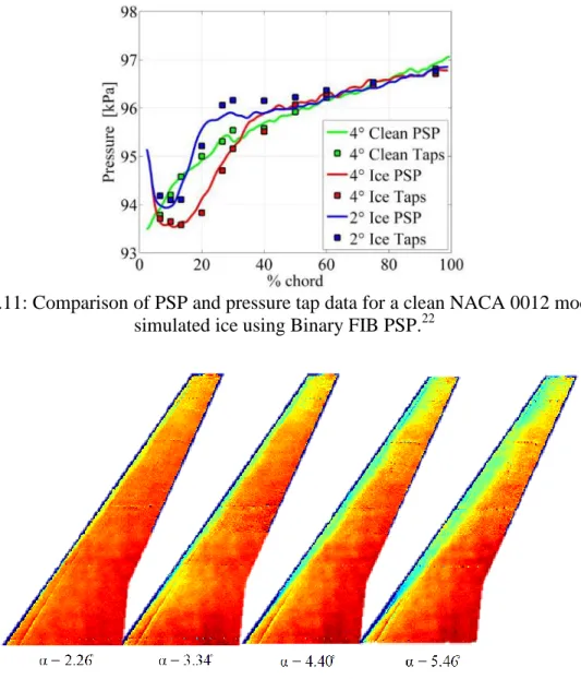
Some work in icing has been performed using PSP as a flow diagnostic. Bencic23 developed a PSP technique to apply the paint directly to an ice accreted model in the IRT. The paint was applied and cured at sub-freezing temperatures, and PSP data acquired in the icing tunnel for two GLC 305 airfoils. It was concluded that PSP could successfully be applied to ice accreted models and that there was excellent agreement between the PSP and pressure tap data. It was also found that the PSP results differed between the iced region of the tested airfoils and the clean aluminum model section downstream of the ice. Ferrigno et al.24 also studied icing using a PSP technique on a NACA 0012 model with simulated rime and glaze ice shapes. It was concluded during that work that PSP is a potentially beneficial technique to obtain pressure data over a surface. This work was performed at low speeds of M ≈ 0.2, proving further that PSP results can be obtained in flows with small pressure gradients. A short study was performed in the UIUC 2ft by 2ft subsonic wind tunnel on a NACA 0012 model with and without an ice shape using binary PSP. This work is recorded by Crafton et al.22 Figure 1.11 shows the published data from this test, where the PSP results qualitatively yield information about the separated flow region behind the ice shape. Diebold et al.25 studied the pressure field of a swept wing, based on the Common Research Model,26 using a radiometric PSP method at low speeds (M ≈ 0.18). The presence and growth of a leading-edge vortex was clearly seen in the results shown in Figure 1.12, providing additional, though mostly qualitative, information about the aerodynamic penalties due to an ice shape that could not be obtained with pressure taps only. This is especially true for a swept wing, where the chordwise pressure distribution is not constant along the span. Diebold et al.25 concluded that PSP was a useful technique for enabling further understanding of a three-dimensional flowfield.
20 Figure 1.11: Comparison of PSP and pressure tap data for a clean NACA 0012 model and
simulated ice using Binary FIB PSP.22
Figure 1.12: PSP data for a swept wing with simulated horn ice shape over an angle of attack range.25
1.3
Motivation
This work was performed in support of the validation of the three-dimensional ice accretion measurement methodology recently developed by NASA. The successful validation of this method with the currently-employed mold and casting process will enable future testing of large-scale ice shapes for the joint swept-wing icing project. The overall project seeks to improve the understanding of all aspects of icing on swept-wings and to obtain high-fidelity experimental icing data. This specific project seeks to aerodynamically
21 demonstrate that ice shapes from the new technique can reasonably replicate the performance of shapes from the mold and casting technique.
The second goal was to further implement the PSP method in the UIUC Aerodynamics Research Lab. A desired objective was to demonstrate the lab’s ability to use PSP as a viable tool for subsonic testing of swept wings to gain high resolution pressure data in three-dimensional flows, through initial testing on an airfoil model. This method has the potential to provide important data on a swept-wing model which are unable to be obtained from discrete pressure taps. The iced-airfoil flowfields studied in this test allow evaluation of the PSP method in a well-understood flowfield. The focus of this study is to jointly validate the newly developed ice shape replication method with the use of the PSP method.
1.4
Objectives and Approach
The objectives of this study are:
- Determine whether ice shapes documented using a 3-D laser scanner and constructed using rapid-protype processes can accurately reproduce the ice-airfoil aerodynamics of ice shapes generated from the accepted NASA mold and casting process.
- Understand how any flowfield differences explain or relate to the discrepancies between aerodynamic data for the two sets of ice shapes.
- Determine how a pressure sensitive paint (PSP) method can be applied to these models to contribute to further understanding their flowfields, as well as how this contribution compares to more traditional surface pressure and flow visualization methods.
These objectives were pursued through experimental aerodynamic testing and comparison of both castings and rapid-prototype shapes on a NACA 23012 airfoil model. This validation test uses an airfoil model since iced-airfoil flowfields and aerodynamics are well understood. Documenting airfoil ice shapes with the newly developed method is a simpler first step than scanning swept-wing ice shapes. Additionally, the two-dimensional model allows the PSP technique to be further understood. That knowledge can then be applied to swept-wing models with more complex flows.
22 The wind tunnel comparison tests include force balance measurements, discrete surface pressure measurements from pressure taps, wake surveys with total pressure probes, surface oil flow visualization, and pressure-sensitive paint (PSP). This variety of experimental techniques allows aerodynamic and flowfield differences between the ice-shapes made from the current mold and casting method and the new 3-D laser scanner technique to be well understood.
This thesis is divided into three main chapters. The first chapter, the Introduction, describes the background necessary to understand the context and motivation of this work. The next chapter, the Experimental Methodology, describes in detail the experimental methods employed to validate the 3-D ice accretion measurement methodology and the facilities in which the tests took place. The last main chapter is the Results and Discussion, where the results from these tests are presented and analyzed. Following that, a Conclusions, Summary, and Recommendations section summarizes the work. Suggestions for future work are also made. The thesis includes appendices with specific descriptions of the PSP post-processing method, the mold and casting method, and measurement uncertainty analysis.
23
Chapter 2
Experimental Methodology
The experimental equipment used and test procedures followed during the course of this work are described in the proceeding chapter. These descriptions include details of the ice shape acquisition methods, the wind tunnel testing facilities, the employed experimental techniques, and the data post-processing techniques.
2.1
Ice Shape Acquisition
The ice accretions used in this study were generated in the NASA Glenn Research Center Icing Research Tunnel (IRT). After each run, the ice accretion was first documented with a digital scan using the 3-D laser scanner and second by making a mold. The molds from this test were sent to the University of Illinois at Urbana-Champaign (UIUC) to make the cast ice shapes used during dry air testing. The digital scans were processed by NASA and used with rapid-prototype processes to make the rapid-prototype ice shapes that are compared to the casting ice shapes as an objective of this work.
2.1.1
NASA Icing Research Tunnel (IRT) Test
The IRT is a closed-return, atmospheric, refrigerated tunnel used for icing research purposes. The airspeed within the 6ft by 9ft test section can vary between 50 and 350 knots and the temperature can be controlled down to -25 degrees Celsius within +/- 0.5 degrees. Upstream of the test section are spray bars that create an icing cloud within the tunnel of supercooled water droplets with median volume diameters between 15 and 50 microns. The icing cloud is about 4.5ft by 6ft centered in the IRT and its water content can be varied from 0.2 to 2.5 g/m3. Models are mounted on a turntable in the test section floor.27
Ice accretions for twelve different icing conditions were generated during testing on a NACA 23012 aluminum model with a chord of 18 inches that spanned the 6ft height of the
24 test section. The conditions were chosen in order to generate ice shapes that correspond to the four classifications defined by Bragg et al.3 as roughness, horn, streamwise, and spanwise ridge. Additionally, the conditions are the same as those used in the tests performed by Busch5 in order to compare data and validate test methods. The NACA 23012 IRT model features a removable leading edge that can be detached along with an ice accretion and placed in a mold box to create a mold. For each of the twelve test cases, the IRT was cooled to the desired temperature and the icing cloud formed for a specified length of time. Once the ice accretion was generated, the tunnel was stopped and documentation of the shape began. Digital photographs were first taken and then the laser scanner method described by Lee et al.28 was performed. The ice was first sprayed with a titanium-dioxide, highly reflective white paint that gives the laser scanner an opaque surface to scan, rather than the transparent and refractive ice. The chosen Romer Absolute arm-based 3-D laser scanner was then used to scan the ice accretion in conjunction with the GeoMagic software.28 Once a sufficient number of data points were collected, the model’s leading-edge section was removed with the ice and placed in a mold box. The mold material was poured into the mold box with the leading edge and ice accretion and left to cure overnight in a refrigerated environment. After curing, the mold was returned to room temperature, the ice melted, and the mold removed from the mold box. All twelve molds were then shipped to the UIUC Aerospace Engineering Research Machine Shop for casting production. During an identical run, the same ice shapes were generated in order for a 2-D tracing of the shape near the center of the model span to be made. The tracing method is one of the IRT’s standard methods of recording two dimensional ice shapes. A heated metal plate with a NACA 23012 cutout is used to melt a small section of ice. The plate is removed and replaced with cardboard with the same NACA 23012 geometry cutout. A pencil is then carefully moved around the ice accretion to record its important features on the cardboard.
2.1.2
Casting Production
The mold material used in the IRT to create the original molds must be able to cure at colder temperatures to ensure that the ice does not melt during pouring and curing. These colder temperatures are typically not within the design temperature range of most molding materials. The specific mold material used in this step of the process was chosen because it
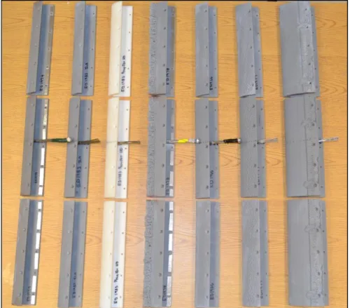
25 is able to cure at cold temperatures. A consequence of using this material is that the resulting mold is extremely stiff and breaks easily when removing a casting. Therefore, the molds needed to be remade of a more durable and flexible material. To do this, master castings of all twelve ice shapes were made using Freeman 1080 Slow Polyurethane Elastomer that was tinted green for visibility. From the twelve master castings, six were chosen to be used in the aerodynamic performance tests. These six master castings are pictured in Figure 2.1. This choice was based on shape uniformity over the span of the casting and so that each classification of ice shape was represented. The digital scans from the 3-D laser scanner were also used in the selection process to ensure that the scanner had successfully captured the features of the ice shape selected. The chosen six master castings were used to create new molds with GT 5092 High Strength Silicone RTV that are more durable than the original molds and are able to be used repeatedly.
Each new mold was used to make four production castings: three test castings and one sacrificial casting. The sacrificial casting was cut at the spanwise location of the pressure taps and traced. This was done in order to obtain a general outline of the ice shape at the tap location and to assist in determining individual tap placement. Each trace was digitized and imported into a CAD program, where the coordinates and orientations of the tap holes were chosen and applied based on the trace geometry. Each of the three test castings were machined to a length of 11 3/16 inches at the spanwise extent chosen earlier and drilled for mounting holes. All three castings were mounted simultaneously on the leading edge of the UIUC NACA 23012 model as shown in Figure 2.2. The edge locations on the test castings were chosen to minimize the discontinuities between adjacent shapes and so the ice was as uniform as possible over the span. One of the three test castings was instrumented with 20 pressure taps at the locations and orientations determined in conjunction with the CAD drawing of the two-dimensional trace. One of the instrumented castings can be viewed close-up in Figure 2.3 and all six sets of completed test castings can be seen in Figure 2.4. The entire casting method is described in more detail in Appendix C.
26
a) b)
c) d)
e) f)
Figure 2.1: Master castings of tested ice shapes, a) ED1974 roughness, b) ED1967 runback (spanwise-ridge), c) ED1978 horn, d) ED1977 streamwise, e) ED1966 streamwise,
f) ED1983 roughness.
Figure 2.2: Three test castings (ED1983 roughness) installed on the NACA 23012 model in the tunnel test section.
27 Figure 2.3: Instrumented test casting (ED1983 roughness).
Figure 2.4: All Test Casting Ice Shapes. From left to right: ED1974 roughness, ED1983 roughness, ED1978 horn, ED1966 streamwise, ED1977 streamwise, and ED1967 runback.
2.1.3
Rapid-Prototype Shape Production
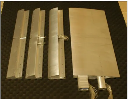
The digital scans acquired by the laser scanner were post-processed by NASA using the method outlined in Lee et al.28 Any holes in the data were filled using the GeoMagic software. The geometry of the UIUC NACA 23012 leading edge and the mounting hole pattern were used with the scans of the ice accretions to create files that could be used with the rapid-prototype processes. Five of the shapes were fabricated using only a
28 stereolithography (SLA) process, while the sixth shape was fabricated using both sterolithography and Polyjet processes. Both stereolithoraphy and Polyjet techniques are rapid-prototype methods. The two different materials and processes were chosen to test the aerodynamic effects of the methods’ differing resolutions. Stereolithography involves building parts in a vat of resin. A laser beam is used to cure the resin in the shape of the part layer by layer. Polyjet involves a jetting head dispensing resin on a building plate layer by layer. The resin is cured immediately using UV light.29 Three identical rapid-prototype segments were made for each shape. These correspond to the same 11 3/16 inches spanwise segment chosen for the castings. The pressure tap locations were chosen prior to fabrication and the holes made as a part of the rapid-prototype process in one of the segments. The final seven sets of rapid-prototype shapes are presented in Figure 2.5.
Figure 2.5: All Test RPM Ice Shapes. From left to right: ED1974 roughness, ED1983 roughness (SLA), ED1983 roughness (PJ), ED1978 horn, ED1966 streamwise, ED1977
29
2.2
Aerodynamic Testing
2.2.1
UIUC Aerodynamics Research Lab Wind Tunnel Facility
The dry-air, aerodynamic wind tunnel testing for the 3-D laser scanner validation was performed at the UIUC subsonic wind tunnel in the Aerodynamics Research Lab. The tunnel is an open-return type with a rectangular 2.8ft by 4ft by 8ft test section. The width and height of the test section increase by 0.5 inches from beginning of the test section to the end in order to account for the growth of the floor boundary layer. The contraction ratio between the inlet and the test section is 7.5:1. The turbulence intensity is kept to below 0.1% at all operating speeds through the presence of flow straighteners, 4 inch honeycomb and four screens, at the tunnel inlet. The tunnel fan can reach rotational speeds of 1200 rpm, which corresponds to about 165 mph or 242 ft/s. The 5-bladed fan is driven by a 125 hp AC motor which is regulated by a variable frequency drive (ABB ACS 800 Low voltage AC drive) and controlled by a Labview code on a personal computer. A schematic of this facility is shown in Figure 2.6.30,31
The test section velocity ( ) is determined from the measurement of the pressure difference between the test section and the settling section ( ) using Bernoulli’s equation. There are four pressure taps each at the tunnel inlet and the beginning of the test section, one on each of the four sides of the tunnel, to measure static pressure. The static pressure taps are pneumatically averaged at each location and the difference measured by both a Setra 239 differential pressure transducer and an Electronically Scanned Pressure (ESP) module. The ESP system will be described in a later section. Using the combination of Bernoulli’s equation in Eq. 2.1 and the conservation of mass for incompressible flow in Eq. 2.2, the velocity in the test section is calculated in Eq. 2.3. In the equations below, is the ambient density. , , and are the settling section cross-sectional area, velocity, and static pressure respectively. , , and are the test section cross-sectional area,
velocity, and static pressure respectively.
(2.1)
30
√ ( )
( ( ) )
(2.3) The ambient density, , is calculated through the ideal gas law in Eq. 2.4, where R is the
specific gas constant for air. The ambient temperature ( ) is measured using an Omega thermocouple, which is situated next to the tunnel. The ambient pressure ( ) is measured using a Setra 270 absolute pressure transducer open to the ambient air around the tunnel.
(2.4)
The dynamic pressure in the test section ( ) is calculated from Eqs. 2.1 and 2.2. Rearranging those two equations and using the definition of dynamic pressure,
, the dynamic pressure can be expressed as shown in Eq. 2.5. The pressure
coefficient can then be calculated using the calculated dynamic pressure value. This equation is stated in Eq. 2.6. ( ) (2.5) [ ( ) ] (2.6)
The Reynolds number based on the model chord (Re) is calculated using Eq. 2.7. Here, the freestream velocity is the test section velocity ( ) and the density is the ambient density ( ). The viscosity constant is calculated using Sutherland’s law in Eq. 2.8. The
reference viscosity coefficient and the reference temperature in Eq. 2.8 are the values for air at freezing conditions, where and . Using the ambient temperature measured by the thermocouple ( ) in Sutherland’s Law, the viscosity coefficient is calculated. The tunnel Labview code held the Reynolds number to within 0.5% of the specified value. The maximum tunnel Reynolds number is 1.5 x 10⁶/ft.
(2.7)
[( ) ⁄
31 Figure 2.6: ARL 3ft by 4ft Subsonic Tunnel.32
2.2.2
Model
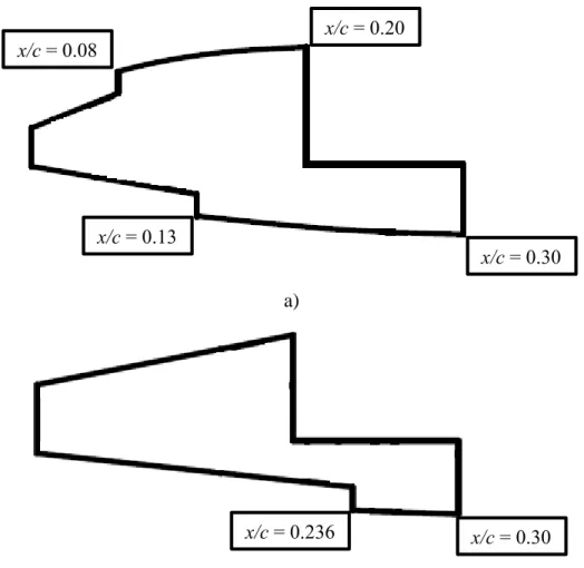
The model used for this testing is an aluminum NACA 23012 airfoil model with an 18 inch chord and 33.563 inch span. This particular model was chosen for this study to compare results with previous work by Busch5 and to be used in conjunction with the IRT model of the same airfoil and chord. There are three interchangeable leading-edge pieces for this model: one clean leading edge and two leading edges used to mount ice shapes. These are shown in Figure 2.7. The model installed in the tunnel with the clean leading edge is pictured in Figure 2.8. The “Appendix C” leading edge is used to mount ice shapes that are representative of accretions formed in the conditions specified in Appendix C to Part 25 of the FAA Federal Aviation Regulations (FARs). The “Super-Cooled Liquid Droplet (SLD)” leading edge is used to mount ice shapes representing accretions formed in SLD conditions or on wings that use leading-edge heating devices, where ice forms further along the chord than in the Appendix C conditions. The seams between the mounted leading edges and the main body of the model are at x/c = 0.30 on the lower surface and x/c = 0.20 on the upper surface. The Appendix C leading edge has the geometry of the clean NACA 23012 airfoil from x/c = 0.13 to x/c = 0.30 on its lower surface and from x/c = 0.08 to x/c = 0.20 on its