FUN3D and USM3D Analysis of the 4th AIAA Propulsion
Aerodynamics Workshop Nozzle Test Case
Michael D. Bozeman Jr.,∗Melissa B. Carter,†and Jan-Reneé Carlson‡ NASA Langley Research Center,
Hampton, VA 23681, USA
This work presents the results of FUN3D and USM3D analyses that were performed for the 4th AIAA Propulsion Aerodynamics Workshop. The workshop was separated into three sections that focus on internal duct flows, nozzle flows, and a special topic of interest. This paper focuses on the nozzle section while an accompanying paper discusses the analyses performed for the internal duct flow section. For the nozzle flow section, the participants were provided with two configurations consisting of a rectangular convergent nozzle with and without an aft-deck. User-generated grids were developed under the guidelines of the workshop for the present analyses. The results show that both solvers compare favorably to the experimental results for the baseline nozzle with the largest differences observed at the lower NPR values. Additionally, both solvers showed favorable agreement with the experimental data for the pressures on the surface of the aft-deck. However, neither solver was able to match the jet flow further downstream for the nozzle with aft-deck configuration. A turbulence model study was conducted to compare the two-equation SST model, SA-QCR model, and two-equation k-kL model (FUN3D only). The results show that the SA-QCR turbulence model was unable to match the experimental results downstream of the nozzle. The k-kL model was shown to better match the experimental data compared to the SST model for most cases simulated using the FUN3D flow solver. Suggestions for future workshops include gridding guidelines similar to those employed for the Drag Prediction Workshop series for the grid refinement study and a reduction in scope to allow for more detailed exploration of the individual problems.
I. Nomenclature
Dh = hydraulic diameter of nozzle exit
k-k L = two-equation kinetic energy - kinetic energy/length-scale product turbulence model
N PR = nozzle pressure ratio,Pt,exit/Pt,∞
Ppitot = pitot pressure
Pt,∞ = freestream total pressure
RAN S = Reynolds Averaged Navier-Stokes
RSM = Reynolds Stress Model
S A = Spalart-Allmaras one-equation turbulence model
SST = Menter Shear Stress Transport two-equation tubulence model
QC R = Quadratic Constitutive Relation
x,y,z = coordinate axes
y+ = dimensionless wall spacing
Z PG = Zero Pressure Gradient
II. Introduction
T
he 4th Propulsion Aerodynamics Workshop (PAW04) was held at the 2018 AIAA Propulsion & Energy Forum inCincinnati, OH. Based on the success of other workshops such as the Drag Prediction Workshop (DPW), the PAW∗Pathways Research Student Trainee, Configuration Aerodynamics Branch, Student Member AIAA. †Aerospace Engineer, Configuration Aerodynamics Branch, Senior Member AIAA.
‡Research Scientist, Computational Aerosciences Branch, Senior Member AIAA.
workshop was created to provide a forum for participants to work on common problems and share experiences. The PAW workshop series was motivated by the challenges associated with accurate predictions of steady and unsteady flows in inlets and nozzles with the goal of stimulating code improvements and enhancing the current state of the art. The workshop series is subdivided into sections focused on the prediction of inlet and nozzle flows along with a special topics section that focuses on current problems of interest. For the inlet section of the workshop series, the main challenge identified was the accurate prediction of flow separation resulting from the offset between the inlet and engine faces in an attempt to make aircraft smaller and more compact [1]. For nozzles, the primary challenge is accurately predicting jet flows over a range of operating conditions with and without integration effects. These problems have proven particularly challenging for Reynolds Averaged Navier-Stokes (RANS) solvers. This paper focuses on NASA Langley’s participation in the nozzle section of PAW04 while an accompanying paper discusses the work performed for the inlet section [2].
The nozzle test cases provided for the PAW04 participants consisted of two converging rectangular nozzles; one with an aft-deck and one without. The aft-deck is representative of highly integrated nozzle configurations typical of fighter-type aircraft. The participants were asked to simulate both nozzles over a range of nozzle pressure ratios (NPRs) and provide both pressure and Mach number values at various locations in the nozzle plume. A common set of grids consisting of coarse, medium, and fine grid refinements for both nozzle configurations were supplied to the participants. These grids were to be used to perform a grid refinement study. Alternatively, the participants were given the option of generating custom grids using provided guidelines. Upon completion of the grid refinement study, the selected grid was to be used to perform an NPR sweep along with a variety of optional studies to examine the impact of geometry changes as well as solver parameters.
For the present work, user-generated grids were created to accommodate some desired grid modifications to be discussed in a later section. This was performed to accomodate some desired modifications to the grids that will be discussed in a later section. Simulations were performed using the NASA Langley developed USM3D and FUN3D flow solvers. This paper will discuss the grid generation procedure, problem setup, and the computational results along with comparisons to experimental data. Finally, recommendations are provided for future PAW workshops based on the authors’ experiences of PAW04.
III. Nozzle Test Case
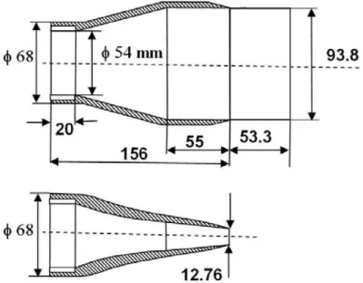
Participants were provided with two nozzle geometries for PAW04. The first geometry is a high-aspect ratio rectangular convergent nozzle, which is referred to as the baseline nozzle geometry. The baseline nozzle consists of a circular to rectangular transition with an exit aspect ratio of 7.35, as illustrated in Figure 1. The second geometry consists of the addition of an aft-deck, measuring 53.3 mm long by 93.8 mm wide by 10 mm thick, to the baseline nozzle. These two nozzle configurations were tested at the Loughborough University High Pressure Nozzle Test Facility [3]. An illustration of the experimental setup for the two nozzle configurations is provided in Figure 2.
A. Test Cases
The participants were provided all required and optional nozzle geometries and test conditions. The required cases consisted of five solutions for each of the two geometries for a total of 10 solutions. For each geometry, the analysis consisted of two steps. The first step was to perform a grid refinement study at a single NPR value of 3.5 using the coarse, medium, and fine grids. Then, based on the results of the grid refinement study, the participants were to select the appropriate grid resolution and simulate additional NPR values of 1.89 and 2.45, where 1.89 represents the theoretical value for the onset of choked flow at the throat of the nozzle.
The optional test cases included additional NPR values and variation in the size of the aft-deck. Additionally, participants were given the option to perform studies to assess the sensitivity of the solution to turbulence model, flux limiter, differencing method, y+, etc. For the present work, only the turbulence model study was performed.
B. Boundary Conditions
Participants were instructed to perform nozzle simulations using static freestream conditions (Mach∼0) and static pressure and temperature values of 14.69 psi and 504◦R, respectively. The inflow to the nozzle was defined by the given total conditions where the total pressure is defined by the NPR and the total temperature defined to be equal to the ambient value of 504◦R.
The experiment included a long, circular supply duct upstream of the nozzle resulting in a relatively thick boundary layer (BL) entering the nozzle. However, the computational domain supplied to the participants started at the nozzle
Fig. 1 Baseline nozzle geometry with measurements.
(a) Baseline nozzle (b) Nozzle with aft-deck
Fig. 2 Experimental setup for nozzle geometries.
entrance. To account for this difference, the participants were provided with estimates of the velocity and total pressure profiles entering the nozzle. The estimated boundary layer profiles were created by applying scaling laws to measured profiles from a previous experiment. The measured profiles corresponded to a nozzle geometry with a supply duct to throat area ratio of 1.56 compared to a value of 1.92 for the nozzle geometry considered here. Also, the measurements were performed for an NPR of 1.57. In order to provide approximate profiles for the given nozzle at the necessary NPR conditions, the measured profiles were scaled based on the assumption of choked flow in the nozzle. For this nozzle test, no turbulence measurements were obtained. However, experimental data measured at the nozzle inlet showed that the BL thickness was relatively constant for all tested NPRs, and the velocity profile closely approximated the classical equilibrium, zero pressure gradient (ZPG) log-law. This indicated that the published data for ZPG boundary layers should provide a reasonable approximation for the turbulence quantities. Finally, the turbulence length scales were estimated based on the smooth wall measurements of the axial integral scale from the work of Antonia [4].
IV. Computational Methods
For this work, the FUN3D and USM3D flow solvers were used. This section discusses the solution strategies employed for the present work including descriptions of the flow solvers, grid generation, and strategy for enforcing the
boundary layer profiles at the inflow boundary. A. FUN3D Flow Solver
FUN3D is an unstructured three-dimensional, implicit, Navier-Stokes solver. A variety of turbulence models are available such as the one-equation Spalart-Allmaras (SA) model [5] with and without the Quadratic Constitutive Relation (QCR) correction [6] and several two-equation models, including Menter’s Shear Stress Transport (SST) model [7] and the k-kL model based on Abdol-Hamid’s closure and Menter’s modifications to Rotta’s two-equation model [8–10]. For this work, Roe’s flux difference splitting [11] was used for the calculation of the inviscid terms. The method for calculation of the Jacobian was the flux function of van Leer [12] with the minmod flux limiter. Also, the SST two-equation model was the primary method for turbulent closure. Other details regarding FUN3D can be found in the manual [13], as well as in the extensive bibliography that is accessible at the FUN3D Web site [14].
B. USM3D Flow Solver
USM3D [15] is a cell-centered, finite-volume Navier-Stokes flow solver that uses multiple flux splitting schemes including Roe’s flux-difference splitting scheme [16] to compute inviscid flux quantities across the faces of the tetrahedral cells. Several options for turbulent closure are available: the one-equation SA model with and without the QCR correction and several two-equation models, including Menter’s SST model. Throughout the study, the minmod limiter was used in order to keep the flow stable and provide consistent results. For the majority of the flow solution cases, the SST turbulence model was used.
C. Grid Generation
Participants were provided with a series of grids for each geometry, both structured and unstructured, to be used for a grid refinement study. Additionally, the participants were given the option of generating custom grids under a provided set of guidelines. For the present work, a new series of grids was generated for the following three reasons: 1) the unstructured grids were provided in mixed-element format, and the version of USM3D used for this work required tetrahedral element grids, 2) some preliminary analysis illustrated some issues with reflection at the farfield boundary of the provided grids indicating that the farfield boundary needed to be moved further downstream of the nozzle exit, and 3) to allow for the addition of an upstream duct. The upstream duct was included to account for the boundary layer entering the nozzle observed in the experiment. This is discussed further in Section IV. D.
The grid generation was performed using Pointwise®v18.2 [17]. Pointwise®is a structured and unstructured grid generator with an intuitive interface and CAD clean-up capabilities. The geometry surface is divided into user-defined computational domains. For each domain, the user can define the point density and spacings on the connectors, which define the outer edges of the computational domains. Additionally, Pointwise®offers the user a variety of metrics for controlling the density of the interior of the domains. For unstructured grids, Pointwise®is capable of generating both mixed-element and all-tetrahedral grids. The boundary layer is resolved using anisotropic tetrahedrals known as T-Rex cells, which can be combined into prisms to generate mixed-element grids. Grid generation is a two-step process consisting of generating the surface grids and volume grids separately. This allows for more control compared to single-step grid generation software. Pointwise® is heavily documented including a variety of tutorials, theory description, and a wide array of scripts available that enable automation of common grid generation problems.
For the present work, Pointwise®was used to generate a mixed-element, coarse grid for each nozzle configuration. The coarse grid was developed with the goal of matching the grid resolution to that of the provided coarse grids. Note that the farfield was extended for the present work, such that matching the total number of cells was not necessary. Instead, the goal was to match the grid resolution on the surface of the nozzle geometry and the plume, which represented the original domain of the provided grids. The farfield was extended downstream to provide ample distance for the plume to expand without reflection at the boundaries. An illustration of the farfield and symmetry plane is provided in Figure 3. Once the coarse grids were generated, the medium and fine grids were created using the gridRefine script available on GitHub. The gridRefine script was developed by Pointwise®and provides an automated way to perform grid refinement based on a user-defined scale factor. The scale factor is uniformly applied to both the connectors and the interior of the domains. For the connectors, the scale factor is applied to refine the spacing constraints and point densities. In the domain interior, the scale factor is applied to the edge lengths of the cells. Additionally, the user has the option of applying the scale factor to y+ to refine the boundary layer. For the present case, y+ was held constant at a desired value of 1 for consistency with the provided grids. A scale factor of 21/4was found to yield comparable
densities to that of the provided grids for this work.
(a) Symmetry plane comparison between provided grids (red) and custom grids (blue)
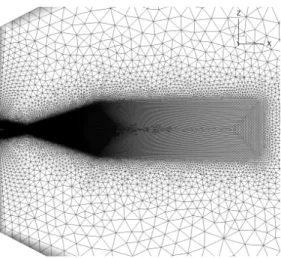
(b) Plume resolution at symmetry plane
Fig. 3 Illustration of the symmetry plane and plume resolution for nozzle grids.
Once the new series of mixed-element grids was generated, an all-tetrahedral series was generated for the USM3D solver. Pointwise®allows the user to choose the type of elements used in the boundary layer when solving the grid volumes. For the mixed-element grids, the boundary layer consists of anisotropic tetrahedrals that are then recombined into prisms. For the all-tetrahedral grids, this recombination step is omitted. The result is that the grids only differ in the types of cells in the boundary layer. An illustration of the mixed-element and tetrahedral-element grids is provided in Figure 4.
(a) Boundary layer resolved with mixed elements for FUN3D solver
(b) Boundary layer resolved with tetrahedral elements for USM3D solver
Fig. 4 Illustration of the differences between boundary layer elements for FUN3D and USM3D grids. Note that since the all-tetrahedral grids do not undergo the recombination step, there are significantly more cells in the boundary layer compared to the mixed-element grids. The number of nodes remains relatively unchanged such that the grid resolution is the same if both grids were used in a node-based solver. However, USM3D not only requires all-tetrahedral grids, but it is also a cell-centered solver. The result is that the USM3D grids are significantly more refined than the FUN3D grids. Because of this, the FUN3D and USM3D results cannot be directly compared and are instead treated as separate analyses. A more valuable comparison between the two solvers could be obtained if the grid
resolution were more closely matched. In previous work, this has been performed by attempting to match the number of cells in the USM3D grids to the number of nodes in the FUN3D grids. However, a single set of grids was provided to the participants regardless of whether the solver being used was node-based or cell-centered. In an effort to be consistent with the workshop, the grids were developed in the manner discussed here. This issue will be partly resolved for future workshops with the release of the mixed-element version of USM3D [18].
1. Baseline Nozzle
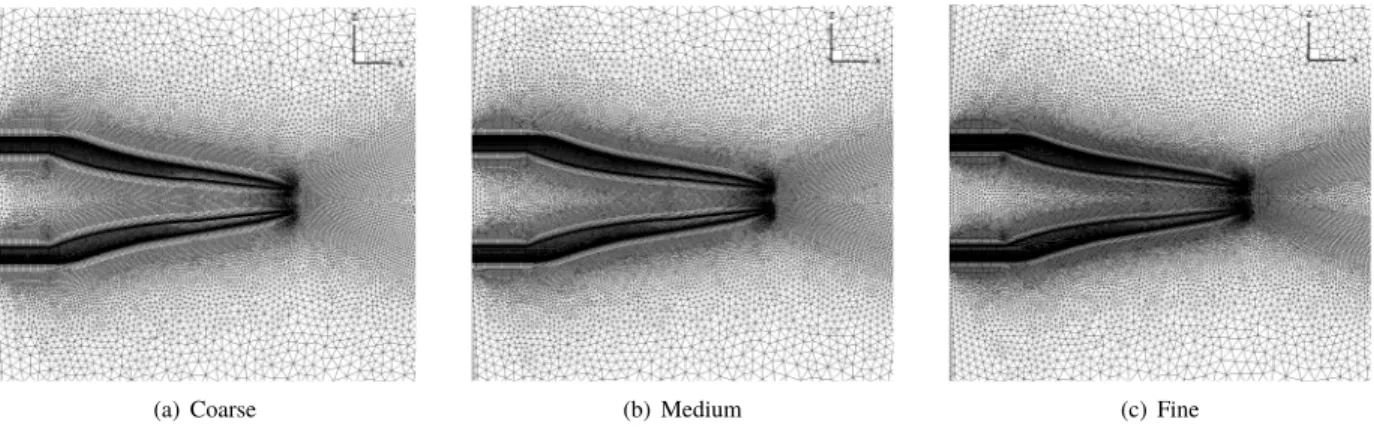
The resulting mixed-element grids for the baseline nozzle cases are illustrated in Figure 5, while the grid resolutions for both FUN3D and USM3D are compared in Table 1. Note that the all-tetrahedral grids are not shown here for conciseness.
(a) Coarse (b) Medium (c) Fine
Fig. 5 Mixed-element grid series for baseline nozzle configuration.
Table 1 Grid resolutions for baseline nozzle configuration. Nodes / Cells (Millions)
Coarse Medium Fine
Mixed-Element Grids 5.786 / 20.849 8.074 / 30.580 11.742 / 46.446 Tetrahedral-Element Grids 5.765 / 34.025 8.011 / 47.359 11.731 / 69.445
2. Nozzle with Aft-Deck
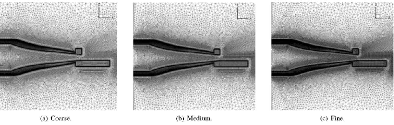
Similarly, the resulting grids for the nozzle with aft-deck configuration are illustrated in Figure 6, with the grid resolutions for both FUN3D and USM3D compared in Table 2.
Table 2 Grid resolutions for nozzle with aft deck configuration. Nodes / Cells (Millions)
Coarse Medium Fine
Mixed-Element Grids 5.834 / 20.878 8.031 / 30.112 11.991 / 47.091 Tetrahedral-Element Grids 5.806 / 34.238 8.042 / 47.511 11.978 / 70.933
(a) Coarse. (b) Medium. (c) Fine.
Fig. 6 Mixed-element grid series for nozzle with aft-deck configuration.
D. Inflow Boundary Conditions
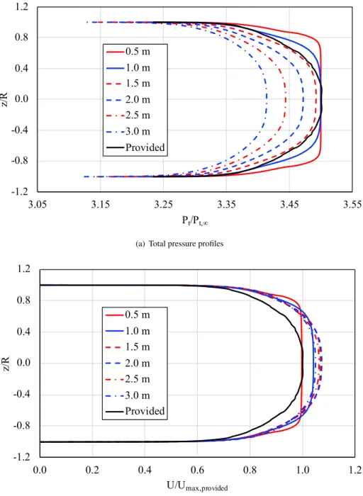
As previously discussed, the participants were provided with approximate boundary layer profiles to enforce at the inflow boundary. For this work, an upstream duct was added to the computational domain to account for the boundary layer entering the nozzle. The upstream duct allows the boundary layer to develop naturally and is more representative of the actual experiment that was conducted. In order to obtain a fully-developed turbulent boundary layer that was representative of the prescribed boundary layer profiles, a study was performed using FUN3D. The study consisted of varying the length of the duct and comparing the predicted boundary layer profiles at the nozzle inlet to the prescribed profiles as illustrated in Figure 7. Note that the study was performed for an NPR value of 3.5 using the coarse grid.
The results illustrated in Figure 7 show that the boundary layer is still developing for duct lengths less that 1.5 meters. This results in a difference in the shape of the profiles compared to the provided profiles. For duct lengths greater than 1.5 meters, the shape of the profiles is relatively unchanged, but the flow experiences greater total pressure loss in the duct. The results provided in Figure 7a show that the total pressure profile is matched closely by the 1.5 meter duct. However, the results provided in Figure 7b show a difference in the velocity profiles. The shapes of the velocity profiles agree fairly well but the maximum velocity predicted by FUN3D is roughly 10% larger than the maximum velocity in the provided profiles. In this case, the FUN3D predicted maximum velocity was assumed to be more accurate than the provided values because the provided values were obtained using simplifying assumptions. One notable assumption was that the boundary layer profiles measured for an NPR value of 1.57 corresponded to a choked flow. According to nozzle theory, choked flow does not occur until an NPR of 1.89. This assumption could lead to a Mach number underprediction in the core flow, which could explain the difference shown here. Based on this observation, a duct length of 1.5 meters was chosen for this work. An illustration of the nozzle geometry with the upstream duct is provided in Figure 8.
-1.2 -0.8 -0.4 0.0 0.4 0.8 1.2 3.05 3.15 3.25 3.35 3.45 3.55 z/ R Pt/Pt,¥ 0.5 m 1.0 m 1.5 m 2.0 m 2.5 m 3.0 m Provided
(a) Total pressure profiles
-1.2 -0.8 -0.4 0.0 0.4 0.8 1.2 0.0 0.2 0.4 0.6 0.8 1.0 1.2 z/ R U/Umax,provided 0.5 m 1.0 m 1.5 m 2.0 m 2.5 m 3.0 m Provided (b) Velocity profiles
Fig. 7 Comparison between FUN3D predicted boundary layer profiles resulting from upstream duct and workshop provided profiles.
1.5 m 0.166 m
E. Convergence
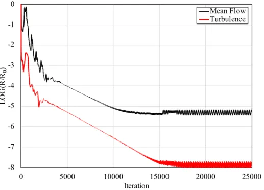
All of the nozzle cases were simulated for a total of 20,000 iterations. The goal in general was to obtain at least three orders of magnitude reduction in the flow residuals. However, for the present work, the solution time was not a limiting factor, and the flow residuals were generally reduced further. An example of the FUN3D convergence history for the baseline nozzle, using the coarse grid, is provided in Figure 9.
-8 -7 -6 -5 -4 -3 -2 -1 0 0 5000 10000 15000 20000 25000 LO G (R /R0 ) Iteration Mean Flow Turbulence
Fig. 9 Baseline nozzle convergence history obtained using FUN3D for the coarse grid at an NPR of 3.5. The convergence history in Figure 9 shows that the mean flow residuals are reduced by more than 5 orders of magnitude and the turbulence residuals are reduced by nearly 8 orders of magnitude. The residuals actually reach a minimum and then proceed to oscillate about the minimum with no further reduction. This type of convergence behavior was typical of all of the simulated cases.
V. Results
The participants were asked to supply a wealth of data for each of the nozzle cases. The data included both Mach number and total pressure values along the centerline of the plume along with both vertical and horizontal profiles at up to 14 downstream locations. The Mach number and total pressure were used to calculate the pitot pressure for comparisons to experimental data. Additionally, the pressure data on the surface of the aft deck were requested for the nozzle with aft-deck configuration. This amount of data would be too overwhelming to include in a single discussion. Therefore, the results presented in this study will only focus on the centerline profiles, vertical and horizontal profiles at axial locations corresponding to 5 and 10 hydraulic diameters downstream of the nozzle exit, and pressure values on the surface of the aft-deck for the nozzle with aft-deck configuration. Also, only the pitot pressure results are provided to allow for comparisons to the experimental data. Note that the participants did not have direct access to these data prior to the workshop. However, the experimental data are included here to add value to the discussion of the results. This section discusses the results at the aforementioned locations obtained from both FUN3D and USM3D for the grid refinement study, NPR sweep, and turbulence model study. The FUN3D and USM3D results are plotted together along with the experimental data for conciseness. However, due to significant differences in grid refinement, there is no intention to draw conclusions about the differences between the two solvers.
A. Grid Refinement Study
The grid refinement study was performed for each of the two nozzle geometries using the coarse, medium, and fine grids discussed in Section IV. C. Note that the participants were instructed to perform the grid refinement study for a single NPR value of 3.5, which was the highest required NPR for the PAW04 analysis cases. The results of the study are presented for each nozzle configuration in the following subsections.
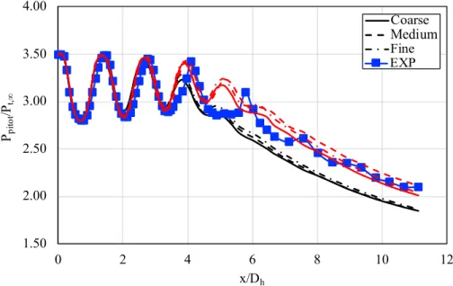
1. Baseline Nozzle 1.50 2.00 2.50 3.00 3.50 4.00 0 2 4 6 8 10 12 Ppi tot /Pt, ¥ x/Dh 0.80 1.05 1.30 1.55 1.80 2.05 0 50 100 150 200 250 Ma ch x (mm) Coarse - FUN3D Medium - FUN3D Fine - FUN3D Coarse - USM3D Medium - USM3D Fine - USM3D 0.80 1.05 1.30 1.55 1.80 2.05 0 50 100 150 200 250 Ma ch x (mm) Coarse - FUN3D Medium - FUN3D Fine - FUN3D Coarse - USM3D Medium - USM3D Fine - USM3D 0.80 1.05 1.30 1.55 1.80 2.05 0 50 100 150 200 250 Ma ch x (mm) Coarse - FUN3D Medium - FUN3D Fine - FUN3D Coarse - USM3D Medium - USM3D Fine - USM3D 1.50 2.00 2.50 3.00 3.50 4.00 0 50 100 150 200 250 Ppitot /Pt, ¥ x (mm) Coarse - FUN3D Medium - FUN3D Fine - FUN3D EXP Coarse - USM3D Medium - USM3D Fine - USM3D
Fig. 10 Grid refinement study results along centerline for baseline nozzle configuration obtained from FUN3D (black), USM3D (red), and experiment (blue).
The results provided in Figure 10 illustrate the pitot pressure normalized by the freestream total pressure along the centerline of the baseline nozzle for the coarse, medium, and fine grids. For both the FUN3D and USM3D flow solvers, there doesn’t appear to be a strong variation with grid refinement. Comparing the predicted results from FUN3D and USM3D to the experimental data, USM3D matches the experimental data very well with the exception of one small region betweenx/Dhvalues of 4 and 6. FUN3D, on the other hand, does a very good job closer to the nozzle exit but begins to deviate from the experimental results around anx/Dhvalue of 4.
The vertical and horizontal profiles atx/Dhvalues of 5 and 10, Figures 11 and 12, illustrate similar trends to those observed for the centerline results. The coarse, medium, and fine grids compare well with very little difference. The overall shape of the pitot pressure profiles is fairly consistent between both FUN3D and USM3D solutions with the main differences being closer to the centerline, where FUN3D predicts lower values of pitot pressure at both axial locations. Comparing the predicted results to the experimental data, both solvers compare reasonably well to the experiment at the location ofx/Dh= 5. FUN3D and USM3D underpredict the vertical jet spreading relative to the experimental data but do a very good job predicting the lateral jet spreading. FUN3D matches the experimental data very well, whereas USM3D overpredicts the centerline values. At the location ofx/Dh = 10, neither solver matches the experimental data. USM3D does a fairly good job capturing the centerline pitot pressure. However, both solvers underpredict the jet spreading in the vertical direction and overpredict the jet spreading in the lateral direction.
0.5 1.0 1.5 2.0 2.5 3.0 3.5 -4.0 -3.0 -2.0 -1.0 0.0 1.0 2.0 3.0 4.0 Ppi tot /Pt, ¥ z/Dh 0.80 1.05 1.30 1.55 1.80 2.05 0 50 100 150 200 250 Ma ch x (mm) Coarse - FUN3D Medium - FUN3D Fine - FUN3D Coarse - USM3D Medium - USM3D Fine - USM3D
0.80
1.05
1.30
1.55
1.80
2.05
0
50
100
150
200
250
Ma chx (mm)
Coarse - FUN3D
Medium - FUN3D
Fine - FUN3D
Coarse - USM3D
Medium - USM3D
Fine - USM3D
0.80 1.05 1.30 1.55 1.80 2.05 0 50 100 150 200 250 Ma ch x (mm) Coarse - FUN3D Medium - FUN3D Fine - FUN3D Coarse - USM3D Medium - USM3D Fine - USM3D 1.50 2.00 2.50 3.00 3.50 4.00 0 50 100 150 200 250 Ppi tot /Pt, ¥ x (mm) Coarse - FUN3D Medium - FUN3D Fine - FUN3D EXP Coarse - USM3D Medium - USM3D Fine - USM3D(a) Pitot pressure profiles as a function ofz/Dh
0.5 1.0 1.5 2.0 2.5 3.0 3.5 -4.0 -3.0 -2.0 -1.0 0.0 1.0 2.0 3.0 4.0 Ppi tot /Pt, ¥ y/Dh 0.80 1.05 1.30 1.55 1.80 2.05 0 50 100 150 200 250 Ma ch x (mm) Coarse - FUN3D Medium - FUN3D Fine - FUN3D Coarse - USM3D Medium - USM3D Fine - USM3D
0.80
1.05
1.30
1.55
1.80
2.05
0
50
100
150
200
250
Ma chx (mm)
Coarse - FUN3D
Medium - FUN3D
Fine - FUN3D
Coarse - USM3D
Medium - USM3D
Fine - USM3D
0.80 1.05 1.30 1.55 1.80 2.05 0 50 100 150 200 250 Ma ch x (mm) Coarse - FUN3D Medium - FUN3D Fine - FUN3D Coarse - USM3D Medium - USM3D Fine - USM3D 1.50 2.00 2.50 3.00 3.50 4.00 0 50 100 150 200 250 Ppi tot /Pt, ¥ x (mm) Coarse - FUN3D Medium - FUN3D Fine - FUN3D EXP Coarse - USM3D Medium - USM3D Fine - USM3D(b) Pitot pressure profiles as a function ofy/Dh
Fig. 11 Grid refinement study results atx/Dh = 5 for baseline nozzle configuration obtained from FUN3D (black), USM3D (red), and experiment (blue).
0.5 1.0 1.5 2.0 2.5 3.0 3.5 -4.0 -3.0 -2.0 -1.0 0.0 1.0 2.0 3.0 4.0 Ppi tot /Pt, ¥ z/Dh 0.80 1.05 1.30 1.55 1.80 2.05 0 50 100 150 200 250 Ma ch x (mm) Coarse - FUN3D Medium - FUN3D Fine - FUN3D Coarse - USM3D Medium - USM3D Fine - USM3D
0.80
1.05
1.30
1.55
1.80
2.05
0
50
100
150
200
250
Ma chx (mm)
Coarse - FUN3D
Medium - FUN3D
Fine - FUN3D
Coarse - USM3D
Medium - USM3D
Fine - USM3D
0.80 1.05 1.30 1.55 1.80 2.05 0 50 100 150 200 250 Ma ch x (mm) Coarse - FUN3D Medium - FUN3D Fine - FUN3D Coarse - USM3D Medium - USM3D Fine - USM3D 1.50 2.00 2.50 3.00 3.50 4.00 0 50 100 150 200 250 Ppi tot /Pt, ¥ x (mm) Coarse - FUN3D Medium - FUN3D Fine - FUN3D EXP Coarse - USM3D Medium - USM3D Fine - USM3D(a) Pitot pressure profiles as a function ofz/Dh
0.5 1.0 1.5 2.0 2.5 3.0 3.5 -4.0 -3.0 -2.0 -1.0 0.0 1.0 2.0 3.0 4.0 Ppi tot /Pt, ¥ y/Dh 0.80 1.05 1.30 1.55 1.80 2.05 0 50 100 150 200 250 Ma ch x (mm) Coarse - FUN3D Medium - FUN3D Fine - FUN3D Coarse - USM3D Medium - USM3D Fine - USM3D
0.80
1.05
1.30
1.55
1.80
2.05
0
50
100
150
200
250
Ma chx (mm)
Coarse - FUN3D
Medium - FUN3D
Fine - FUN3D
Coarse - USM3D
Medium - USM3D
Fine - USM3D
0.80 1.05 1.30 1.55 1.80 2.05 0 50 100 150 200 250 Ma ch x (mm) Coarse - FUN3D Medium - FUN3D Fine - FUN3D Coarse - USM3D Medium - USM3D Fine - USM3D 1.50 2.00 2.50 3.00 3.50 4.00 0 50 100 150 200 250 Ppi tot /Pt, ¥ x (mm) Coarse - FUN3D Medium - FUN3D Fine - FUN3D EXP Coarse - USM3D Medium - USM3D Fine - USM3D(b) Pitot pressure profiles as a function ofy/Dh
Fig. 12 Grid refinement study results atx/Dh = 10 for baseline nozzle configuration obtained from FUN3D (black), USM3D (red), and experiment (blue).
2. Nozzle with Aft-Deck 1.50 2.00 2.50 3.00 3.50 4.00 0 2 4 6 8 10 12 Ppi tot /Pt, ¥ x/Dh 0.80 1.05 1.30 1.55 1.80 2.05 0 50 100 150 200 250 Ma ch x (mm) Coarse - FUN3D Medium - FUN3D Fine - FUN3D Coarse - USM3D Medium - USM3D Fine - USM3D
0.80
1.05
1.30
1.55
1.80
2.05
0
50
100
150
200
250
Ma chx (mm)
Coarse - FUN3D
Medium - FUN3D
Fine - FUN3D
Coarse - USM3D
Medium - USM3D
Fine - USM3D
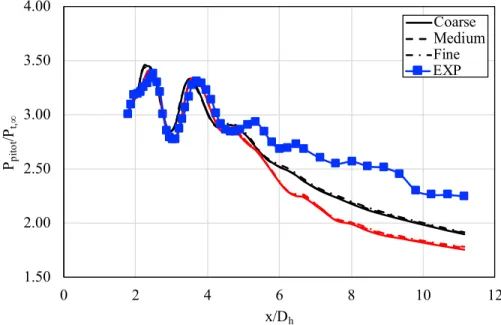
0.80 1.05 1.30 1.55 1.80 2.05 0 50 100 150 200 250 Ma ch x (mm) Coarse - FUN3D Medium - FUN3D Fine - FUN3D Coarse - USM3D Medium - USM3D Fine - USM3D 1.50 2.00 2.50 3.00 3.50 4.00 0 50 100 150 200 250 Ppi tot /Pt, ¥ x (mm) Coarse - FUN3D Medium - FUN3D Fine - FUN3D EXP Coarse - USM3D Medium - USM3D Fine - USM3DFig. 13 Grid refinement study results along centerline for nozzle with aft-deck configuration obtained from FUN3D (black), USM3D (red), and experiment (blue).
Similarly, the results of the grid refinement study for the nozzle with aft-deck configuration are illustrated in Figures 13, 14, and 15. The results show that grid refinement has even less of an effect than observed for the baseline nozzle configuration. Comparing the centerline pitot pressure predictions to the experimental data, both solvers compare well to the experimental data closer to the exit of the nozzle. However, neither solver captures the experimental data downstream ofx/Dh= 5. This is also observed in the vertical and horizontal pitot pressure profiles provided in Figures 14 and 15. Atx/Dh= 5, both solvers do a fairly good job at predicting the vertical and lateral jet spreading. For the vertical profile results, the experimental data exhibit a noticeable bias in the negative z-direction due to the presence of the aft-deck. The FUN3D and USM3D results also show this bias but to a lesser extent. For the lateral profile results, both flow solvers accurately predict the lateral jet spreading. However, while both solvers predict the overall shape very well, neither solver is able to exactly match the lateral data near the centerline. Atx/Dh= 10, the predictions are noticeably worse compared to the experimental data. Both solvers underpredict the vertical jet spreading. However, USM3D is able to closely match the peak pitot pressure value. For the lateral profile results, both solvers underpredict the lateral jet spreading. Also, the experimental results show that the centerline experiences less deceleration relative to the flow on either side. This can be seen by the shifting of the peak pitot pressure from roughlyy/Dh= -1 and 1 for the data atx/Dh= 5 toy/Dh= 0 for the data atx/Dh= 10. However, neither flow solver predicts this behavior atx/Dh= 10. This result explains the differences observed in the centerline pitot pressure predictions relative to the experimental data in Figure 13.
Finally, the predicted static pressures on the aft-deck are compared to experimental data for the coarse, medium, and fine grids in Figure 16. The experimental results show that the flow accelerates at the nozzle exit. The pressure then remains relatively constant fromx/Dh= 1 to 1.8 where a shock forms causing a sudden increase in the pressure. The pressure distribution then show a slight increase between the last two points. Similar to the previous results, the results show little difference for the coarse, medium, and fine grids. The FUN3D predictions do show some slight differences between x/Dh = 1.5 and 2, which is in the vicinity of the shock. Both flow solvers overpredict the pressure at the nozzle exit but compare favorably to the experimental data up to the flow in the vicinity of the shock. The USM3D solver accurately predicts the location of the shock but overpredicts the shock strength relative to the experimental data. FUN3D predicts the shock to occur roughly 0.3 hydraulic diameters upstream of the experimental value and also overpredicts the shock strength.
0.5 1.0 1.5 2.0 2.5 3.0 3.5 -4.0 -3.0 -2.0 -1.0 0.0 1.0 2.0 3.0 4.0 Ppi tot /Pt, ¥ z/Dh 0.80 1.05 1.30 1.55 1.80 2.05 0 50 100 150 200 250 Ma ch x (mm) Coarse - FUN3D Medium - FUN3D Fine - FUN3D Coarse - USM3D Medium - USM3D Fine - USM3D 0.80 1.05 1.30 1.55 1.80 2.05 0 50 100 150 200 250 Ma ch x (mm) Coarse - FUN3D Medium - FUN3D Fine - FUN3D Coarse - USM3D Medium - USM3D Fine - USM3D 0.80 1.05 1.30 1.55 1.80 2.05 0 50 100 150 200 250 Ma ch x (mm) Coarse - FUN3D Medium - FUN3D Fine - FUN3D Coarse - USM3D Medium - USM3D Fine - USM3D 1.50 2.00 2.50 3.00 3.50 4.00 0 50 100 150 200 250 Ppitot /Pt, ¥ x (mm) Coarse - FUN3D Medium - FUN3D Fine - FUN3D EXP Coarse - USM3D Medium - USM3D Fine - USM3D
(a) Pitot pressure profiles as a function ofz/Dh
0.5 1.0 1.5 2.0 2.5 3.0 3.5 -4.0 -3.0 -2.0 -1.0 0.0 1.0 2.0 3.0 4.0 Ppi tot /Pt, ¥ y/Dh 0.80 1.05 1.30 1.55 1.80 2.05 0 50 100 150 200 250 Ma ch x (mm) Coarse - FUN3D Medium - FUN3D Fine - FUN3D Coarse - USM3D Medium - USM3D Fine - USM3D 0.80 1.05 1.30 1.55 1.80 2.05 0 50 100 150 200 250 Ma ch x (mm) Coarse - FUN3D Medium - FUN3D Fine - FUN3D Coarse - USM3D Medium - USM3D Fine - USM3D 0.80 1.05 1.30 1.55 1.80 2.05 0 50 100 150 200 250 Ma ch x (mm) Coarse - FUN3D Medium - FUN3D Fine - FUN3D Coarse - USM3D Medium - USM3D Fine - USM3D 1.50 2.00 2.50 3.00 3.50 4.00 0 50 100 150 200 250 Ppitot /Pt, ¥ x (mm) Coarse - FUN3D Medium - FUN3D Fine - FUN3D EXP Coarse - USM3D Medium - USM3D Fine - USM3D
(b) Pitot pressure profiles as a function ofy/Dh
Fig. 14 Grid refinement study results atx/Dh= 5 for nozzle with aft-deck configuration obtained from FUN3D (black), USM3D (red), and experiment (blue).
0.5 1.0 1.5 2.0 2.5 3.0 3.5 -4.0 -3.0 -2.0 -1.0 0.0 1.0 2.0 3.0 4.0 Ppi tot /Pt, ¥ z/Dh 0.80 1.05 1.30 1.55 1.80 2.05 0 50 100 150 200 250 Ma ch x (mm) Coarse - FUN3D Medium - FUN3D Fine - FUN3D Coarse - USM3D Medium - USM3D Fine - USM3D 0.80 1.05 1.30 1.55 1.80 2.05 0 50 100 150 200 250 Ma ch x (mm) Coarse - FUN3D Medium - FUN3D Fine - FUN3D Coarse - USM3D Medium - USM3D Fine - USM3D 0.80 1.05 1.30 1.55 1.80 2.05 0 50 100 150 200 250 Ma ch x (mm) Coarse - FUN3D Medium - FUN3D Fine - FUN3D Coarse - USM3D Medium - USM3D Fine - USM3D 1.50 2.00 2.50 3.00 3.50 4.00 0 50 100 150 200 250 Ppitot /Pt, ¥ x (mm) Coarse - FUN3D Medium - FUN3D Fine - FUN3D EXP Coarse - USM3D Medium - USM3D Fine - USM3D
(a) Pitot pressure profiles as a function ofz/Dh
0.5 1.0 1.5 2.0 2.5 3.0 3.5 -4.0 -3.0 -2.0 -1.0 0.0 1.0 2.0 3.0 4.0 Ppi tot /Pt, ¥ y/Dh 0.80 1.05 1.30 1.55 1.80 2.05 0 50 100 150 200 250 Ma ch x (mm) Coarse - FUN3D Medium - FUN3D Fine - FUN3D Coarse - USM3D Medium - USM3D Fine - USM3D 0.80 1.05 1.30 1.55 1.80 2.05 0 50 100 150 200 250 Ma ch x (mm) Coarse - FUN3D Medium - FUN3D Fine - FUN3D Coarse - USM3D Medium - USM3D Fine - USM3D 0.80 1.05 1.30 1.55 1.80 2.05 0 50 100 150 200 250 Ma ch x (mm) Coarse - FUN3D Medium - FUN3D Fine - FUN3D Coarse - USM3D Medium - USM3D Fine - USM3D 1.50 2.00 2.50 3.00 3.50 4.00 0 50 100 150 200 250 Ppitot /Pt, ¥ x (mm) Coarse - FUN3D Medium - FUN3D Fine - FUN3D EXP Coarse - USM3D Medium - USM3D Fine - USM3D
(b) Pitot pressure profiles as a function ofy/Dh
Fig. 15 Grid refinement study results atx/Dh= 10 for nozzle w/ aft-deck configuration obtained from FUN3D (black), USM3D (red), and experiment (blue).
0.0 0.2 0.4 0.6 0.8 1.0 1.2 1.4 1.6 1.8 2.0 0 0.5 1 1.5 2 2.5 P/ Pt,¥ x/Dh 0.80 1.05 1.30 1.55 1.80 2.05 0 50 100 150 200 250 Ma ch x (mm) Coarse - FUN3D Medium - FUN3D Fine - FUN3D Coarse - USM3D Medium - USM3D Fine - USM3D
0.80
1.05
1.30
1.55
1.80
2.05
0
50
100
150
200
250
Ma chx (mm)
Coarse - FUN3D
Medium - FUN3D
Fine - FUN3D
Coarse - USM3D
Medium - USM3D
Fine - USM3D
0.80 1.05 1.30 1.55 1.80 2.05 0 50 100 150 200 250 Ma ch x (mm) Coarse - FUN3D Medium - FUN3D Fine - FUN3D Coarse - USM3D Medium - USM3D Fine - USM3D 1.50 2.00 2.50 3.00 3.50 4.00 0 50 100 150 200 250 Ppi tot /Pt, ¥ x (mm) Coarse - FUN3D Medium - FUN3D Fine - FUN3D EXP Coarse - USM3D Medium - USM3D Fine - USM3DFig. 16 Surface pressure on aft-deck for nozzle with aft-deck as a function of grid refinement obtained from FUN3D (black), USM3D (red), and experiment (blue).
3. Grid Refinement Summary
The results presented in this section show that there is not a significant variation in the predicted pitot pressure for the coarse, medium, and fine grids for either flow solver. However, this may be attributed to the limited separation in the grid refinements. As a result, no concrete conclusions can be made about grid refinement here. The fine grid was selected for the remainder of the nozzle analyses. Based on the results discussed in this section, the coarse grid was likely sufficient, but the time savings between the coarse and fine grids was not enough to warrant the lesser grid refinement.
Future workshops should aim to provide grids with a larger variation in grid refinement. The DPW workshops consider significantly larger ranges of grid refinements. For example, the finest mixed element grid considered in the DPW-5 had roughly 62 times the number of nodes as the coarsest grid refinement [19]. For the present workshop, the finest grid had roughly 2 times the number of nodes as the coarsest grid.
B. PAW04 Required Cases
The participants were asked to further simulate NPR values of 1.89 and 2.45 using the grid selected from the grid refinement study. The results for all three NPR values required for the PAW04 participants are presented in the following sections. Note that all of the solutions presented in this section were produced using the fine grid.
1. Baseline Nozzle
The results illustrated in Figure 17 compare the pitot pressure predicted by both the FUN3D and USM3D flow solvers as well as the experimentally measured values for the three NPR values. The results for an NPR value of 3.5 have already been discussed but are included here for reference. For both NPR values of 1.89 and 2.45, the computational results compare well to the experimental data closer to the nozzle exit. However, the computational results begin to differ near anx/Dh value of 3. The results show that both FUN3D and USM3D underpredict the experimentally measured pitot pressure further downstream. The results in Figure 18 show that qualitatively both solvers do a good job predicting the experimental results with the exception of the USM3D results for an NPR of 3.5. FUN3D matches the experimental results very well at an NPR value of 2.45 but underpredicts the pitot pressure for an NPR value of 1.89. USM3D overpredicts the pitot pressure for an NPR of 2.45 and underpredicts for an NPR value of 1.89. For the vertical and lateral results corresponding to anx/Dhvalue of 10, neither solver is able to match the vertical jet spreading for an
1.00 1.50 2.00 2.50 3.00 3.50 4.00 0 2 4 6 8 10 12
P
pitot/P
t, ¥ x/Dh0.50
0.75
1.00
1.25
1.50
1.75
2.00
0
50
100
150
200
250
Ma chx (mm)
NPR = 1.89 - FUN3D
NPR = 2.45 - FUN3D
NPR = 3.5 - FUN3D
NPR = 1.89 - USM3D
NPR = 2.45 - USM3D
NPR = 3.5 - USM3D
0.50
0.75
1.00
1.25
1.50
1.75
2.00
0
50
100
150
200
250
Ma chx (mm)
NPR = 1.89 - FUN3D
NPR = 2.45 - FUN3D
NPR = 3.5 - FUN3D
NPR = 1.89 - USM3D
NPR = 2.45 - USM3D
NPR = 3.5 - USM3D
0.50
0.75
1.00
1.25
1.50
1.75
2.00
0
50
100
150
200
250
Ma chx (mm)
NPR = 1.89 - FUN3D
NPR = 2.45 - FUN3D
NPR = 3.5 - FUN3D
NPR = 1.89 - USM3D
NPR = 2.45 - USM3D
NPR = 3.5 - USM3D
1.00 1.50 2.00 2.50 3.00 3.50 4.00 0 50 100 150 200 250P
pi tot/P
t, ¥ x (mm)Fig. 17 NPR sweep results along centerline for baseline configuration obtained from FUN3D (black), USM3D (red), and experiment (blue).
NPR value of 2.45. However, both solvers appear to match the vertical jet spreading for the case of an NPR value of 1.89 while underpredicting the peak pitot pressure. For the lateral results, the trends observed from the computational results are different than those observed for the experimental results. The experimental results show very little difference in the lateral jet spreading between NPR values of 3.5 and 2.45 with large differences in peak pitot pressure. Then, larger jet spreading in the lateral direction at an NPR value of 1.89 with an even lower peak pitot pressure. The computational results capture the trend of decreasing peak values of pitot pressure with decreasing NPR. However, the computational results show decreased jet spreading in the lateral direction with decreasing NPR. So the increase in lateral spreading at an NPR of 1.89 is not captured by either solver.
0.50 1.00 1.50 2.00 2.50 3.00 3.50 -4.0 -3.0 -2.0 -1.0 0.0 1.0 2.0 3.0 4.0 Ppitot /Pt, ¥ z/Dh
0.50
0.75
1.00
1.25
1.50
1.75
2.00
0
50
100
150
200
250
Ma chx (mm)
NPR = 1.89 - FUN3D
NPR = 2.45 - FUN3D
NPR = 3.5 - FUN3D
NPR = 1.89 - USM3D
NPR = 2.45 - USM3D
NPR = 3.5 - USM3D
0.50
0.75
1.00
1.25
1.50
1.75
2.00
0
50
100
150
200
250
Ma chx (mm)
NPR = 1.89 - FUN3D
NPR = 2.45 - FUN3D
NPR = 3.5 - FUN3D
NPR = 1.89 - USM3D
NPR = 2.45 - USM3D
NPR = 3.5 - USM3D
0.50
0.75
1.00
1.25
1.50
1.75
2.00
0
50
100
150
200
250
Ma chx (mm)
NPR = 1.89 - FUN3D
NPR = 2.45 - FUN3D
NPR = 3.5 - FUN3D
NPR = 1.89 - USM3D
NPR = 2.45 - USM3D
NPR = 3.5 - USM3D
1.00 1.50 2.00 2.50 3.00 3.50 4.00 0 50 100 150 200 250P
pi tot/P
t, ¥ x (mm)(a) Pitot pressure profiles as a function ofz/Dh
0.50 1.00 1.50 2.00 2.50 3.00 3.50 -4.0 -3.0 -2.0 -1.0 0.0 1.0 2.0 3.0 4.0 Ppi tot /Pt, ¥ y/Dh
0.50
0.75
1.00
1.25
1.50
1.75
2.00
0
50
100
150
200
250
Ma chx (mm)
NPR = 1.89 - FUN3D
NPR = 2.45 - FUN3D
NPR = 3.5 - FUN3D
NPR = 1.89 - USM3D
NPR = 2.45 - USM3D
NPR = 3.5 - USM3D
0.50
0.75
1.00
1.25
1.50
1.75
2.00
0
50
100
150
200
250
Ma chx (mm)
NPR = 1.89 - FUN3D
NPR = 2.45 - FUN3D
NPR = 3.5 - FUN3D
NPR = 1.89 - USM3D
NPR = 2.45 - USM3D
NPR = 3.5 - USM3D
0.50
0.75
1.00
1.25
1.50
1.75
2.00
0
50
100
150
200
250
Ma chx (mm)
NPR = 1.89 - FUN3D
NPR = 2.45 - FUN3D
NPR = 3.5 - FUN3D
NPR = 1.89 - USM3D
NPR = 2.45 - USM3D
NPR = 3.5 - USM3D
1.00 1.50 2.00 2.50 3.00 3.50 4.00 0 50 100 150 200 250P
pi tot/P
t, ¥ x (mm)(b) Pitot pressure profiles as a function ofy/Dh
Fig. 18 NPR sweep results atx/Dh= 5 for baseline nozzle configuration obtained from FUN3D (black), USM3D (red), and experiment (blue).
0.50 1.00 1.50 2.00 2.50 3.00 3.50 -4.0 -3.0 -2.0 -1.0 0.0 1.0 2.0 3.0 4.0 Ppi tot /Pt, ¥ z/Dh
0.50
0.75
1.00
1.25
1.50
1.75
2.00
0
50
100
150
200
250
Ma chx (mm)
NPR = 1.89 - FUN3D
NPR = 2.45 - FUN3D
NPR = 3.5 - FUN3D
NPR = 1.89 - USM3D
NPR = 2.45 - USM3D
NPR = 3.5 - USM3D
0.50
0.75
1.00
1.25
1.50
1.75
2.00
0
50
100
150
200
250
Ma chx (mm)
NPR = 1.89 - FUN3D
NPR = 2.45 - FUN3D
NPR = 3.5 - FUN3D
NPR = 1.89 - USM3D
NPR = 2.45 - USM3D
NPR = 3.5 - USM3D
0.50
0.75
1.00
1.25
1.50
1.75
2.00
0
50
100
150
200
250
Ma chx (mm)
NPR = 1.89 - FUN3D
NPR = 2.45 - FUN3D
NPR = 3.5 - FUN3D
NPR = 1.89 - USM3D
NPR = 2.45 - USM3D
NPR = 3.5 - USM3D
1.00 1.50 2.00 2.50 3.00 3.50 4.00 0 50 100 150 200 250P
pitot/P
t, ¥ x (mm)(a) Pitot pressure profiles as a function ofz/Dh
0.50 1.00 1.50 2.00 2.50 3.00 3.50 -4.0 -3.0 -2.0 -1.0 0.0 1.0 2.0 3.0 4.0 Ppi tot /Pt, ¥ y/Dh
0.50
0.75
1.00
1.25
1.50
1.75
2.00
0
50
100
150
200
250
Ma chx (mm)
NPR = 1.89 - FUN3D
NPR = 2.45 - FUN3D
NPR = 3.5 - FUN3D
NPR = 1.89 - USM3D
NPR = 2.45 - USM3D
NPR = 3.5 - USM3D
0.50
0.75
1.00
1.25
1.50
1.75
2.00
0
50
100
150
200
250
Ma chx (mm)
NPR = 1.89 - FUN3D
NPR = 2.45 - FUN3D
NPR = 3.5 - FUN3D
NPR = 1.89 - USM3D
NPR = 2.45 - USM3D
NPR = 3.5 - USM3D
0.50
0.75
1.00
1.25
1.50
1.75
2.00
0
50
100
150
200
250
Ma chx (mm)
NPR = 1.89 - FUN3D
NPR = 2.45 - FUN3D
NPR = 3.5 - FUN3D
NPR = 1.89 - USM3D
NPR = 2.45 - USM3D
NPR = 3.5 - USM3D
1.00 1.50 2.00 2.50 3.00 3.50 4.00 0 50 100 150 200 250P
pi tot/P
t, ¥ x (mm)(b) Pitot pressure profiles as a function ofy/Dh
Fig. 19 NPR sweep results at x/Dh = 10 for baseline nozzle configuration obtained from FUN3D (black), USM3D (red), and experiment (blue).
2. Nozzle with Aft-Deck 1.00 1.50 2.00 2.50 3.00 3.50 4.00 0 2 4 6 8 10 12
P
pitot/P
t, ¥ x/Dh0.50
0.75
1.00
1.25
1.50
1.75
2.00
0
50
100
150
200
250
Ma chx (mm)
NPR = 1.89 - FUN3D
NPR = 2.45 - FUN3D
NPR = 3.5 - FUN3D
NPR = 1.89 - USM3D
NPR = 2.45 - USM3D
NPR = 3.5 - USM3D
0.50
0.75
1.00
1.25
1.50
1.75
2.00
0
50
100
150
200
250
Ma chx (mm)
NPR = 1.89 - FUN3D
NPR = 2.45 - FUN3D
NPR = 3.5 - FUN3D
NPR = 1.89 - USM3D
NPR = 2.45 - USM3D
NPR = 3.5 - USM3D
0.50
0.75
1.00
1.25
1.50
1.75
2.00
0
50
100
150
200
250
Ma chx (mm)
NPR = 1.89 - FUN3D
NPR = 2.45 - FUN3D
NPR = 3.5 - FUN3D
NPR = 1.89 - USM3D
NPR = 2.45 - USM3D
NPR = 3.5 - USM3D
1.00 1.50 2.00 2.50 3.00 3.50 4.00 0 50 100 150 200 250P
pitot/P
t, ¥ x (mm)Fig. 20 NPR sweep results along centerline for nozzle with aft-deck configuration obtained from FUN3D (black), USM3D (red), and experiment (blue).
The centerline results, for the nozzle with aft-deck, illustrated in Figure 20, show similar trends for all three NPR values. The computational results show good agreement from the end of the aft deck up untilx/Dh = 4. The one exception is the USM3D results corresponding to an NPR value of 1.89 where the computational results and experimental results match very well over the entire range ofx/Dhvalues. Another interesting result here is that the predictions appear to match the experiment better as the NPR value is decreased from 3.5 to 1.89, which is completely opposite from the observations from the baseline configuration. The results atx/Dh= 5 also show favorable agreement between the computational and experimental results. FUN3D and USM3D have a tendency to underpredict the pitot pressure relative to the experimental data, but the overall trends are predicted very well by both solvers. Note that both solvers underpredict the vertical spreading in the negative z-direction for the case of an NPR value of 3.5. For the results at
x/Dh= 10, the comparisons show fairly significant differences between the computational and experimental results. This was already discussed for the case of an NPR of 3.5. Overall, FUN3D and USM3D capture the experimental trends for decreasing values of NPR very well. Both solvers also match very well with the experimental data for an NPR value of 1.89. However, neither solver accurately captures the vertical location of the peak pitot pressure from the experimental results for an NPR of 2.45. This contributes to the large differences between pitot pressures observed at the centerline location. This is further illustrated in the lateral profile results atx/Dh= 10. Finally, the comparisons of the static pressures on the aft-deck are provided in Figure 23. Note that the computational results are also shown for an NPR value of 1.89, but the experimental results were not available for this NPR value. The experimental results for an NPR of 2.45 show that the shock on the aft-deck is closer to the nozzle exit and weaker relative to the case of an NPR value of 3.5. Similar to the observations for an NPR of 3.5, both solvers show differences in the vicinity of the shock. FUN3D predicts the shock to be further upstream than USM3D or the experiment, which leads to differences in the static pressure values upstream and downstream of the shock. USM3D accurately captures the location of the shock once again and does a fairly good job of predicting the shock strength relative to the experimental data. However, the USM3D predicted static pressures deviate from the experimental values just downstream of the shock but then match the experimental results well downstream ofx/Dh= 2. For the case of an NPR value of 1.89, both computational results show that there is no shock on the aft-deck for this case. This leads to relatively flat profiles. But again, no experimental data were provided for this NPR value so no concrete conclusions can be made for this condition.
0.5 1.0 1.5 2.0 2.5 3.0 3.5 -4.0 -3.0 -2.0 -1.0 0.0 1.0 2.0 3.0 4.0 Ppi tot /Pt, ¥ z/Dh 0.50 0.75 1.00 1.25 1.50 1.75 2.00 0 50 100 150 200 250 Ma ch x (mm) NPR = 1.89 - FUN3D NPR = 2.45 - FUN3D NPR = 3.5 - FUN3D NPR = 1.89 - USM3D NPR = 2.45 - USM3D NPR = 3.5 - USM3D 0.50 0.75 1.00 1.25 1.50 1.75 2.00 0 50 100 150 200 250 Ma ch x (mm) NPR = 1.89 - FUN3D NPR = 2.45 - FUN3D NPR = 3.5 - FUN3D NPR = 1.89 - USM3D NPR = 2.45 - USM3D NPR = 3.5 - USM3D 0.50 0.75 1.00 1.25 1.50 1.75 2.00 0 50 100 150 200 250 Ma ch x (mm) NPR = 1.89 - FUN3D NPR = 2.45 - FUN3D NPR = 3.5 - FUN3D NPR = 1.89 - USM3D NPR = 2.45 - USM3D NPR = 3.5 - USM3D 1.00 1.50 2.00 2.50 3.00 3.50 4.00 0 50 100 150 200 250
P
pitot/P
t, ¥ x (mm) (a) Pitot pressure profiles as a function ofz/Dh0.5 1.0 1.5 2.0 2.5 3.0 3.5 -4.0 -3.0 -2.0 -1.0 0.0 1.0 2.0 3.0 4.0 Ppi tot /Pt, ¥ y/Dh 0.50 0.75 1.00 1.25 1.50 1.75 2.00 0 50 100 150 200 250 Ma ch x (mm) NPR = 1.89 - FUN3D NPR = 2.45 - FUN3D NPR = 3.5 - FUN3D NPR = 1.89 - USM3D NPR = 2.45 - USM3D NPR = 3.5 - USM3D 0.50 0.75 1.00 1.25 1.50 1.75 2.00 0 50 100 150 200 250 Ma ch x (mm) NPR = 1.89 - FUN3D NPR = 2.45 - FUN3D NPR = 3.5 - FUN3D NPR = 1.89 - USM3D NPR = 2.45 - USM3D NPR = 3.5 - USM3D 0.50 0.75 1.00 1.25 1.50 1.75 2.00 0 50 100 150 200 250 Ma ch x (mm) NPR = 1.89 - FUN3D NPR = 2.45 - FUN3D NPR = 3.5 - FUN3D NPR = 1.89 - USM3D NPR = 2.45 - USM3D NPR = 3.5 - USM3D 1.00 1.50 2.00 2.50 3.00 3.50 4.00 0 50 100 150 200 250
P
pitot/P
t, ¥ x (mm)(b) Pitot pressure profiles as a function ofy/Dh
Fig. 21 NPR sweep results atx/Dh = 5 for nozzle with aft-deck configuration obtained from FUN3D (black), USM3D (red), and experiment (blue).
0.5 1.0 1.5 2.0 2.5 3.0 3.5 -4.0 -3.0 -2.0 -1.0 0.0 1.0 2.0 3.0 4.0 Ppi tot /Pt, ¥ z/Dh 0.50 0.75 1.00 1.25 1.50 1.75 2.00 0 50 100 150 200 250 Ma ch x (mm) NPR = 1.89 - FUN3D NPR = 2.45 - FUN3D NPR = 3.5 - FUN3D NPR = 1.89 - USM3D NPR = 2.45 - USM3D NPR = 3.5 - USM3D 0.50 0.75 1.00 1.25 1.50 1.75 2.00 0 50 100 150 200 250 Ma ch x (mm) NPR = 1.89 - FUN3D NPR = 2.45 - FUN3D NPR = 3.5 - FUN3D NPR = 1.89 - USM3D NPR = 2.45 - USM3D NPR = 3.5 - USM3D 0.50 0.75 1.00 1.25 1.50 1.75 2.00 0 50 100 150 200 250 Ma ch x (mm) NPR = 1.89 - FUN3D NPR = 2.45 - FUN3D NPR = 3.5 - FUN3D NPR = 1.89 - USM3D NPR = 2.45 - USM3D NPR = 3.5 - USM3D 1.00 1.50 2.00 2.50 3.00 3.50 4.00 0 50 100 150 200 250
P
pitot/P
t, ¥ x (mm)(a) Pitot pressure profiles as a function ofz/Dh
0.5 1.0 1.5 2.0 2.5 3.0 3.5 -4.0 -3.0 -2.0 -1.0 0.0 1.0 2.0 3.0 4.0 Ppi tot /Pt, ¥ y/Dh 0.50 0.75 1.00 1.25 1.50 1.75 2.00 0 50 100 150 200 250 Ma ch x (mm) NPR = 1.89 - FUN3D NPR = 2.45 - FUN3D NPR = 3.5 - FUN3D NPR = 1.89 - USM3D NPR = 2.45 - USM3D NPR = 3.5 - USM3D 0.50 0.75 1.00 1.25 1.50 1.75 2.00 0 50 100 150 200 250 Ma ch x (mm) NPR = 1.89 - FUN3D NPR = 2.45 - FUN3D NPR = 3.5 - FUN3D NPR = 1.89 - USM3D NPR = 2.45 - USM3D NPR = 3.5 - USM3D 0.50 0.75 1.00 1.25 1.50 1.75 2.00 0 50 100 150 200 250 Ma ch x (mm) NPR = 1.89 - FUN3D NPR = 2.45 - FUN3D NPR = 3.5 - FUN3D NPR = 1.89 - USM3D NPR = 2.45 - USM3D NPR = 3.5 - USM3D 1.00 1.50 2.00 2.50 3.00 3.50 4.00 0 50 100 150 200 250
P
pitot/P
t, ¥ x (mm)(b) Pitot pressure profiles as a function ofy/Dh
Fig. 22 NPR sweep results atx/Dh= 10 for nozzle with aft-deck configuration obtained from FUN3D (black), USM3D (red), and experiment (blue).
0.0 0.2 0.4 0.6 0.8 1.0 1.2 1.4 1.6 1.8 2.0 0 0.5 1 1.5 2 2.5 P/ Pt,¥ x/Dh
0.50
0.75
1.00
1.25
1.50
1.75
2.00
0
50
100
150
200
250
Ma chx (mm)
NPR = 1.89 - FUN3D
NPR = 2.45 - FUN3D
NPR = 3.5 - FUN3D
NPR = 1.89 - USM3D
NPR = 2.45 - USM3D
NPR = 3.5 - USM3D
0.50
0.75
1.00
1.25
1.50
1.75
2.00
0
50
100
150
200
250
Ma chx (mm)
NPR = 1.89 - FUN3D
NPR = 2.45 - FUN3D
NPR = 3.5 - FUN3D
NPR = 1.89 - USM3D
NPR = 2.45 - USM3D
NPR = 3.5 - USM3D
0.50
0.75
1.00
1.25
1.50
1.75
2.00
0
50
100
150
200
250
Ma chx (mm)
NPR = 1.89 - FUN3D
NPR = 2.45 - FUN3D
NPR = 3.5 - FUN3D
NPR = 1.89 - USM3D
NPR = 2.45 - USM3D
NPR = 3.5 - USM3D
1.00 1.50 2.00 2.50 3.00 3.50 4.00 0 50 100 150 200 250P
pitot/P
t, ¥ x (mm)Fig. 23 Surface pressure on deck for nozzle with aft-deck as a function of NPR obtained from FUN3D (black), USM3D (red), and experiment (blue).
3. NPR Sweep Results Summary
For the baseline configuration, the computational results tend to show larger differences relative to the experimental results as the NPR value decreases. The opposite trend is observed for the nozzle with an aft-deck configuration. The static pressure value comparison on the aft-deck showed that both solvers do a fairly good job matching the experimental data for both NPR values considered with the exception of some differences in the vicinity of the observed shocks. C. Turbulence Model Study
In addition to the required test cases, PAW04 participants were encouraged to perform parameter studies of their choosing. For this work, a turbulence model study was performed using both the FUN3D and USM3D solvers. All of the results discussed so far in this paper have employed the SST two-equation turbulence model. For the turbulence model study, the SA one-equation turbulence model with the QCR Reynolds stress model (RSM) was employed for both the FUN3D and USM3D solvers. The SA-QCR turbulence model has shown to perform well for problems involving corner flows, which are present inside the nozzle configurations for the present work. However, SA one-equation models have historically had issues with accurately predicting jet flows. Additionally, the k-kL two-equation turbulence model was employed in FUN3D; it has not yet been implemented in the USM3D solver. The k-kL turbulence model was developed at the NASA Langley Research Center and has been extensively validated for jet flows. The following sections discuss the results of the turbulence model study that was performed for both the baseline nozzle and nozzle with aft-deck configurations. Note that all comparisons provided are for the case of an NPR value of 3.5 using the fine grid. 1. Baseline Nozzle
The results of the turbulence model study, Figures 24 - 26, show that the SA-QCR model does not compare as well as the two-equation models for either solver. For the FUN3D flow solver, the SA-QCR model drastically underpredicts the centerline pitot pressure downstream ofx/Dh= 5. The opposite is observed for the SA-QCR predictions obtained from USM3D. The k-kL turbulence model results compares better to the experimental data than any of the other turbulence models for FUN3D. In fact, the k-kL turbulence model results approach the SST results obtained by USM3D. The results at a location ofx/Dh= 5 in Figure 25 show that the vertical jet spreading doesn’t exhibit significant sensitivity to the turbulence model. However, the two-equation turbulence models do have a tendency to overpredict the peak pitot pressure relative to the experimental values. The lateral results show that the SA-QCR model overpredicts the
1.50 2.00 2.50 3.00 3.50 4.00 0 2 4 6 8 10 12
P
pitot/P
t, ¥ x/Dh1.50
2.00
2.50
3.00
3.50
4.00
0
50
100
150
200
250
P
pi tot/P
t, ¥ x (mm)SST
SA-QCR
K-kL
EXP
SA-QCR
SST
SST
SA-QCR
k-kL
EXP
Fig. 24 Turbulence model results along centerline for baseline nozzle configuration obtained from FUN3D (black), USM3D (red), and experiment (blue).
lateral jet spreading for both solvers. For FUN3D, the SA-QCR results qualitatively capture the shape of the plume in the lateral direction. However, the peak pitot pressure values on the edges are overpredicted and the centerline value is underpredicted. For USM3D, the SA-QCR overpredicts the pitot pressure over the entire range ofy/Dh values. Interestingly, the SST prediction obtained from FUN3D appears to match the experiment the best at this location. At
x/Dh= 10, the results in Figure 26 show variation in the results for the different turbulence models. All of the turbulence models underpredict the vertical jet spreading and overpredict the lateral jet spreading. Again, the k-kL turbulence model appears to be the best performer for FUN3D at this location, providing comparable predictions to the SST results obtained from USM3D. Again, the USM3D and FUN3D results cannot be compared directly for this work due to the differences in grid refinement. However, it is interesting that the FUN3D results produced using the k-kL turbulence match closely with the USM3D results using the SST turbulence model with a much finer grid resolution.
0.5 1.0 1.5 2.0 2.5 3.0 3.5 -4.0 -3.0 -2.0 -1.0 0.0 1.0 2.0 3.0 4.0 Ppi tot /Pt, ¥ z/Dh
1.50
2.00
2.50
3.00
3.50
4.00
0
50
100
150
200
250
P
pi tot/P
t, ¥ x (mm)SST
SA-QCR
K-kL
EXP
SA-QCR
SST
SST
SA-QCR
k-kL
EXP
(a) Pitot pressure profiles as a function ofz/Dh
0.5 1.0 1.5 2.0 2.5 3.0 3.5 -4.0 -3.0 -2.0 -1.0 0.0 1.0 2.0 3.0 4.0 Ppi tot /Pt, ¥ y/Dh
1.50
2.00
2.50
3.00
3.50
4.00
0
50
100
150
200
250
P
pi tot/P
t, ¥ x (mm)SST
SA-QCR
K-kL
EXP
SA-QCR
SST
SST
SA-QCR
k-kL
EXP
(b) Pitot pressure profiles as a function ofy/Dh
Fig. 25 Turbulence model study results atx/Dh = 5 for baseline nozzle configuration obtained from FUN3D (black), USM3D (red), and experiment (blue).
0.5 1.0 1.5 2.0 2.5 3.0 3.5 -4.0 -3.0 -2.0 -1.0 0.0 1.0 2.0 3.0 4.0 Ppi tot /Pt, ¥ z/Dh
1.50
2.00
2.50
3.00
3.50
4.00
0
50
100
150
200
250
P
pi tot/P
t, ¥ x (mm)SST
SA-QCR
K-kL
EXP
SA-QCR
SST
SST
SA-QCR
k-kL
EXP
(a) Pitot pressure profiles as a function ofz/Dh
0.5 1.0 1.5 2.0 2.5 3.0 3.5 -4.0 -3.0 -2.0 -1.0 0.0 1.0 2.0 3.0 4.0 Ppi tot /Pt, ¥ y/Dh
1.50
2.00
2.50
3.00
3.50
4.00
0
50
100
150
200
250
P
pi tot/P
t, ¥ x (mm)SST
SA-QCR
K-kL
EXP
SA-QCR
SST
SST
SA-QCR
k-kL
EXP
(b) Pitot pressure profiles as a function ofy/Dh
Fig. 26 Turbulence model study results atx/Dh= 10 for baseline nozzle configuration obtained from FUN3D (black), USM3D (red), and experiment (blue).
2. Nozzle with Aft-Deck 1.25 1.75 2.25 2.75 3.25 3.75 0 2 4 6 8 10 12
P
pitot/P
t, ¥ x/Dh1.50
2.00
2.50
3.00
3.50
4.00
0
50
100
150
200
250
P
pi tot/P
t, ¥ x (mm)SST
SA-QCR
K-kL
EXP
SA-QCR
SST
SST
SA-QCR
k-kL
EXP
Fig. 27 Turbulence model study results along centerline for nozzle with aft-deck configuration obtained from FUN3D (black), USM3D (red), and experiment (blue).
The results provided in Figure 27 show that the SA-QCR model drastically underpredicts the pitot pressure downstream. In fact, all of the FUN3D and USM3D predictions underpredict the centerline pitot pressure downstream ofx/Dh = 5. The k-kL turbulence model additionally does not show any benefit over the SST model for this case. These observations are also true for the vertical and lateral profiles atx/Dh= 5, shown in Figure 28. However, the SA-QCR prediction obtained from USM3D actually compares very well to the SST result with the exception of the centerline location, where it underpredicts the pitot pressure. Atx/Dh= 10, the results in Figure 29 show that the SA-QCR predictions obtained from FUN3D again drastically underpredict the pitot pressure. Interestingly, the SA-QCR results obtained from USM3D appear to predict the vertical jet spreading better than any of the other solutions. It is also interesting that the SA-QCR results obtained from USM3D for the both the lateral and vertical profiles compare to the SST results much better than for FUN3D. Again, this is potentially due to grid refinement since the FUN3D grid is much less refined. The k-kL results do not differ very much from the SST results for FUN3D. For the vertical profile, the only discernable difference between the k-kL and SST predictions from FUN3D is the peak pitot pressure, which is predicted to be larger by the k-kL turbulence model. For the lateral profiles, the k-kL model actually does a better job capturing the lateral spread compared to the SST model. Finally, the predicted static pressure values on the aft-deck provided in Figure 30 show that all of the turbulence models do a good job upstream of the shock location. The SA-QCR prediction obtained from FUN3D predicts the shock location to be slightly further downstream relative to the SST model. The same observation is true for the SA-QCR results obtained from USM3D. The k-kL model results accurately predict the shock location and compare very well to the SST model results obtained from USM3D.
0.5 1.0 1.5 2.0 2.5 3.0 3.5 -4.0 -3.0 -2.0 -1.0 0.0 1.0 2.0 3.0 4.0 Ppi tot /Pt, ¥ z/Dh
1.50
2.00
2.50
3.00
3.50
4.00
0
50
100
150
200
250
P
pi tot/P
t, ¥ x (mm)SST
SA-QCR
K-kL
EXP
SA-QCR
SST
SST
SA-QCR
k-kL
EXP
(a) Pitot pressure profiles as a function ofz/Dh
0.5 1.0 1.5 2.0 2.5 3.0 3.5 -4.0 -3.0 -2.0 -1.0 0.0 1.0 2.0 3.0 4.0 Ppitot /Pt, ¥ y/Dh
1.50
2.00
2.50
3.00
3.50
4.00
0
50
100
150
200
250
P
pi tot/P
t, ¥ x (mm)SST
SA-QCR
K-kL
EXP
SA-QCR
SST
SST
SA-QCR
k-kL
EXP
(b) Pitot pressure profiles as a function ofy/Dh
Fig. 28 Turbulence model study results at x/Dh = 5 for nozzle with aft-deck configuration obtained from FUN3D (black), USM3D (red), and experiment (blue).
0.5 1.0 1.5 2.0 2.5 3.0 3.5 -4.0 -3.0 -2.0 -1.0 0.0 1.0 2.0 3.0 4.0 Ppitot /Pt, ¥ z/Dh
1.50
2.00
2.50
3.00
3.50
4.00
0
50
100
150
200
250
P
pi tot/P
t, ¥ x (mm)SST
SA-QCR
K-kL
EXP
SA-QCR
SST
SST
SA-QCR
k-kL
EXP
(a) Pitot pressure profiles as a function ofz/Dh
0.5 1.0 1.5 2.0 2.5 3.0 3.5 -4.0 -3.0 -2.0 -1.0 0.0 1.0 2.0 3.0 4.0 Ppi tot /Pt, ¥ y/Dh
1.50
2.00
2.50
3.00
3.50
4.00
0
50
100
150
200
250
P
pi tot/P
t, ¥ x (mm)SST
SA-QCR
K-kL
EXP
SA-QCR
SST
SST
SA-QCR
k-kL
EXP
(b) Pitot pressure profiles as a function ofy/Dh
Fig. 29 Turbulence model study results at x/Dh = 10 for nozzle with aft-deck configuration obtained from FUN3D (black), USM3D (red), and experiment (blue).
0.0 0.2 0.4 0.6 0.8 1.0 1.2 1.4 1.6 1.8 2.0 0.0 0.5 1.0 1.5 2.0 2.5 P/ Pt,¥ x/Dh
1.50
2.00
2.50
3.00
3.50
4.00
0
50
100
150
200
250
P
pi tot/P
t, ¥ x (mm)SST
SA-QCR
K-kL
EXP
SA-QCR
SST
SST
SA-QCR
k-kL
EXP
Fig. 30 Surface pressure on deck for nozzle with aft-deck as a function of turbulence model obtained from FUN3D (black), USM3D (red), and experiment (blue).
3. Summary of Turbulence Model Study
The results provided in the previous discussion show that there is no definitive answer as to which turbulence model is best for these problems. However, a few observations can be made. The first observation is that the SA-QCR turbulence model does not perform well for the jet flow predictions downstream of the nozzle. Another observation is that the k-kL turbulence model performs better than the SST turbulence model for the cases shown here. And in some cases, the k-kL predictions are comparable to the SST predictions obtained from USM3D with a much finer grid. Future work will test the k-kL model on a grid with higher resolution in FUN3D. Additionally, there are plans to implement the k-kL turbulence model into the USM3D flow solver in the future.
D. Summary and Conclusions
This paper presented the FUN3D and USM3D analyses that were performed for the nozzle configurations in participation of the 4th AIAA Propulsion Aerodynamics Workshop. The participants were provided with two nozzle geometries; a baseline nozzle and a nozzle with an aft-deck. This work consisted of a grid generation exercise to accomodate the USM3D flow solver, to eliminate issues at the farfield boundary, and to allow for the inclusion of an upstream duct, which was necessary to model the boundary layer from the supply duct in the experiment. The performed analyses included a grid refinement study, NPR sweep, and turbulence model study. The grid refinement study illustrated very little differences between the predictions for the coarse, medium, and fine grids. This is likely due to the very close spacing in the grid resolutions, which is potentially an area of improvement for the future workshops. Rather significant differences were observed between the FUN3D and USM3D predictions. However, this is potentially due, in part, to the large grid differences between the two solvers. This issue will be partially mitigated for future workshops with the release of the mixed-element version of USM3D. Comparisons to the experimental data show that both FUN3D and USM3D do a fairly good job for the baseline configuration. Observations from the vertical and lateral profiles at two axial locations show that both solvers tend to underpredict the spreading in the z-direction and overpredict the spreading in the y-direction further downstream. However, neither solver is able to accurately predict the jet flow downstream ofx/Dh= 5 for the nozzle with aft-deck configuration. Observations from the vertical and lateral profiles for this configuration show that both solvers do a fairly good job predicting the lateral and vertical jet spreading atx/Dh= 5. However, at the axial location ofx/Dh = 10, both solvers underpredict the spreading in the negative z-direction caused by the influence of the aft-deck. Likewise, neither solver captures the centerline behavior that is observed for the lateral profile. Finally, the static pressures on the aft-deck were compared to the experimental