CLIMATE OVER PAST MILLENNIA

CLIMATE OVER PAST MILLENNIA

Received 20 October 2003; revised 4 February 2004; accepted 17 February 2004; published 6 May 2004.

[1] We review evidence for climate change over the past several millennia from instrumental and high-resolution climate ‘‘proxy’’ data sources and climate modeling studies. We focus on changes over the past 1 to 2 millennia. We assess reconstructions and modeling studies analyzing a number of different climate fields, including atmospheric circulation diagnostics, precipitation, and drought. We devote particular attention to proxy-based reconstructions of temperature patterns in past centuries, which place recent large-scale warming in an appropriate longer-term context. Our assessment affirms the conclusion that late 20th century warmth is unprecedented at hemispheric and, likely, global scales. There is more tentative evidence that particular modes of climate variability, such as the El Nin˜o/Southern Oscillation and the North Atlantic Oscillation, may have exhibited late 20th century behavior that is anomalous in a long-term context. Regional conclusions, particularly for the Southern Hemisphere and parts of the tropics where high-resolution proxy data are sparse, are more circumspect. The

dramatic differences between regional and hemispheric/ global past trends, and the distinction between changes in surface temperature and precipitation/drought fields, underscore the limited utility in the use of terms such as the ‘‘Little Ice Age’’ and ‘‘Medieval Warm Period’’ for describing past climate epochs during the last millennium. Comparison of empirical evidence with proxy-based reconstructions demonstrates that natural factors appear to explain relatively well the major surface temperature changes of the past millennium through the 19th century (including hemispheric means and some spatial patterns). Only anthropogenic forcing of climate, however, can explain the recent anomalous warming in the late 20th century. INDEX TERMS: 3344 Meteorology and Atmospheric Dynamics: Paleoclimatology; 3309 Meteorology and Atmospheric Dynamics: Climatology (1620); 1620 Global Change: Climate dynamics (3309); 3394 Meteorology and Atmospheric Dynamics: Instruments and techniques; 3354 Meteorology and Atmospheric Dynamics: Precipitation (1854);KEYWORDS:climate

Citation: Jones, P. D., and M. E. Mann (2004), Climate over past millennia,Rev. Geophys.,42, RG2002, doi:10.1029/2003RG000143.

P. D. Jones

Climatic Research Unit

School of Environmental Sciences University of East Anglia

Norwich, UK

M. E. Mann

Department of Environmental Sciences University of Virginia

Charlottesville, Virginia, USA

CONTENTS

1. Introduction and Motivation... 2

1.1. Climate of the Late Holocene ... 2

1.2. Past One to Two Millennia ... 2

1.3. Comparison of Models and Observations... 3

2. Paleoclimate ‘‘Proxy’’ Data... 3

2.1. Instrumental Climate Data... 4

2.2. Historical Documentary Records ... 6

2.3. Tree Ring Records... 8

2.4. Coral Records ... 8

2.5. Ice Core Records ... 9

2.6. Speleothems ... 10

2.7. Varved Lake and Ocean Sediment Records... 10

2.8. Boreholes ... 10

2.9. Glacial Evidence... 11

2.10. Other Proxy Records ... 11

3. Proxy Climate Reconstructions ... 12

3.1. Calibration of Proxy Data ... 12

3.2. Climate Field Reconstruction Approaches... 14

3.3. Multiproxy Reconstructions ... 17

4. Climate Record of the Past Two Millennia ... 18

4.1. Inferences From Instrumental Climate Data and Model Simulations ... 18

4.2. Large-Scale Temperature Changes ... 19

4.3. Large-Scale Hydroclimatic/Moisture Changes ... 21

4.4. Regional Circulation Patterns ... 22

4.4.1. ENSO ... 22

4.4.2. PDO... 24

4.4.3. NAO/AO ... 24

5. Physical Explanations of Past Observed Changes... 24

5.1. Forcing Factors ... 25

5.1.1. Solar Irradiance Forcing ... 25

5.1.2. Volcanic Aerosol Forcing ... 26

5.1.3. Greenhouse Gas Forcing ... 27

5.1.4. Sulphate Aerosol Forcing ... 27

5.1.5. Land Use Change Forcing... 27

5.2. Modeling of Past Climate Changes ... 27

5.3. Model/Data Intercomparison... 29

6. Future Directions: Where Do We Go From Here? ... 30

7. Conclusions and Summary... 31

Copyright 2004 by the American Geophysical Union. 8755-1209/04/2003RG000143$15.00

Reviews of Geophysics, 42, RG2002 / 2004 1 of 42 Paper number 2003RG000143 RG2002

1. INTRODUCTION AND MOTIVATION

[2] Climate varies on all timescales, from years to dec-ades to millennia to millions and billions of years. This climate variability can arise from a number of factors, some external to the climate system others internal to the system [Bradley, 1999; Ruddiman, 2001]. Any improvements in our ability to predict future climate changes are most likely to result from a better understanding of the workings of the climate system as a whole. Such an understanding can, in turn, best be achieved through a greater ability to document and explain, from a fundamental dynamical point of view, observed past variations. Instrumental meteorological records can only assess large-scale (hemispheric and global) climate changes over roughly the past 100 – 150 years, while more regionally limited data (e.g., in Europe) are available back to the early 18th century. Improved knowledge of past large-scale climate changes should enable recent, potentially anomalous, climate change to be placed in a longer-term context. Information from other data sources and/or climate models is thus necessary for insights into climate variability on multicentury and longer timescales. In this review we document the range of information available from paleo-climatic data sources and modeling studies to inform our understanding of climate variability on centennial to mil-lennial timescales. We emphasize climate variations during the past few millennia (the late Holocene), the period that is most relevant to assessing the potential uniqueness of recent climate changes and the projected changes in the 21st century.

1.1. Climate of the Late Holocene

[3] The Pleistocene climate epoch was marked by major ‘‘glacial/interglacial’’ oscillations in global ice volume that occurred on timescales of tens to hundreds of millennia. These oscillations appear to have been governed by similar timescale changes in the distribution of insolation over the Earth’s surface related to long-term changes in the orbital position of the Earth relative to the Sun. The most recent glacial period culminated about 21,000 years ago (the Last Glacial Maximum) when continental ice sheets extended well into the midlatitudes of North America and Europe. Global annual mean temperatures were probably about 4C colder than the mid-20th century, with larger cooling at higher latitudes and little or no cooling over large parts of the tropical oceans [e.g., Ruddiman, 2001]. This glacial period terminated somewhat abruptly, 12,000 years ago. The climate appears to have exhibited less dramatic, but nonetheless significant, variability on centennial and mil-lennial timescales during the subsequent interglacial period, referred to as the ‘‘Holocene,’’ within which we currently reside. During the early millennia of the Holocene, atmo-spheric circulation, surface temperature, and precipitation patterns appear to have been substantially altered from the present day, with evidence, for example, of ancient lakes in what is now the Sahara [Street and Grove, 1979]. During the ‘‘mid-Holocene’’ of 5000 – 6000 years ago, surface temperatures appear to have been milder in some parts of

the globe, particularly in the extratropics of the Northern Hemisphere during summer [see Webb and Wigley, 1985]. This has given rise to the use of the descriptor ‘‘Holocene Optimum’’ sometimes used to characterize this period. There is still considerable uncertainty, however, with regard to the relative global, annual mean warmth at this time, because much of the evidence for warmer conditions comes from the extratropics and appears biased toward warm season conditions. The orbitally induced insolation changes likely favored warmer high-latitude summers but cooler winters and slightly cooler tropics, with any net hemispheric- or global-scale changes representing a subtle competition between these seasonally and spatially hetero-geneous changes [Hewitt, 1998; Kitoh and Murakami, 2002; Liu et al., 2003] and seasonally specific (e.g., vegetation-albedo) feedbacks [e.g., Ganopolski et al., 1998]. Recent modeling studies suggest that mid-Holocene surface temperatures for annual and global means may actually have been cooler than those of the mid-20th century, even though extratropical summers were likely somewhat warmer [Kitoh and Murakami, 2002].

[4] Extratropical summer temperatures appear to have cooled over the subsequent four millennia [e.g., Matthes, 1939]. This period, sometimes referred to as the ‘‘Neo-glacial’’ because it was punctuated with periods of glacial advance (and of glacial retreat) of extratropical mountain glaciers [e.g.,Matthes, 1939;Porter and Denton, 1967], was reminiscent of, though far more modest than, a full glacial period during the Pleistocene epoch. Orbital influences likely influenced large-scale climate over this time frame through an interaction with the monsoon and El Nin˜o–

Southern Oscillation(ENSO) phenomena [e.g.,Joussaume et al., 1999;Bush, 1999;Liu et al., 2000;Clement et al., 2000]. (Italicized terms are defined in the glossary, after the main text.) Evidence regarding the actual nature of changes in ENSO over past millennia [Sandweiss et al., 1996, 2001;

Tudhope et al., 2001; Koutavas et al., 2002; Stott et al., 2002] is controversial [DeVries et al., 1997;Trenberth and Otto-Bliesner, 2003]. This is due to the paucity of evidence, uncertainty concerning the influences in the proxies used, or the inability of the proxy records to resolve true (interannual) El Nin˜o variability. Recent evidence also suggests that human-induced land use changes influencing methane and CO2production may have begun to influence the climate over the past several millennia [Ruddiman, 2003].

1.2. Past One to Two Millennia

[5] When we restrict our attention to the more limited interval of the past one to two millennia, a period that can be referred to as the ‘‘late Holocene’’ [Williams and Wigley, 1983], the principal boundary conditions on the climate (e.g., Earth orbital geometry and global ice mass) have not changed appreciably. The variations in climate observed over this time frame are likely therefore to be representative of the natural climate variability that might be expected over the present century in the absence of any human influence. Placing modern climate change, including recent global-scale warming, in a longer-term context can thus help

establish the importance of anthropogenic forcing (human-generated greenhouse gas concentration increases and aero-sol production) on recent past and future climate changes.

[6] Much recent work has focused on the changes during this shorter time interval, over which widespread high-resolution, precisely dated proxy records are available for large regions of the Northern Hemisphere and some parts of theSouthern Hemisphere(SH) [Jones et al., 2001a;Mann, 2001a, 2002a;Mann and Jones, 2003]. This paper reviews the evidence for changes over the past one to two millennia. Details of the available proxy climate data and how they are assimilated into multiple-proxy-based (multiproxy) climate reconstructions are discussed in sections 2 and 3. Interpre-tations of the proxies, in terms of climate change over the past one to two millennia, are discussed in section 4.

1.3. Comparison of Models and Observations

[7] Evidence of past climate change should not be interpreted in isolation. Comparison of climate model sim-ulations and empirical paleoclimatic data can greatly en-hance our understanding of the climate system. Such studies help to assess the role of external forcing, including natural (e.g., volcanic and solar radiative) and anthropogenic (greenhouse gas and sulphate aerosol) influences, and natural, internal variability (e.g., natural changes in the El Nin˜o – Southern Oscillation and century- or millennial-scale natural oscillations in the coupled ocean-atmosphere sys-tem). Models can help us determine how we might have expected the climate system to have changed given past changes in boundary conditions and forcings, which we can compare to inferences derived from paleoclimatic data.

[8] Internal variability generated in coupled ocean-atmo-sphere models can be verified against the long-term vari-ability evident in proxy-based temperature reconstructions of the past millennium [Mann et al., 1995;Barnett et al., 1996, 1999; Jones et al., 1998; Braganza et al., 2003;

Covey et al., 2003; Bell et al., 2003]. Natural external forcing by volcanoes, the Sun [Lean et al., 1995; Crowley and Kim, 1996, 1999;Cubasch et al., 1997;Overpeck et al., 1997; Mann et al., 1998a; Damon and Peristykh, 1999;

Free and Robock, 1999; Rind et al., 1999; Crowley, 2000;

Gerber et al., 2003; Bertrand et al., 2002; Shindell et al., 2001, 2003; Waple et al., 2002; Bauer et al., 2003], and, particularly during the 19th and 20th centuries, human land use changes [Govindasamy et al., 2001;Bauer et al., 2003] all appear to have played significant roles. Comparisons of climate models with estimated forcing changes and proxy climate reconstructions can therefore provide constraints on the sensitivity of the climate to radiative forcing [Crowley and Kim, 1999; Crowley, 2000; Gerber et al., 2003;

Bertrand et al., 2002; Bauer et al., 2003]. Additionally,

general circulation model (GCM) simulations of climate can provide details of the spatial response of the climate to forcing [Cubasch et al., 1997;Waple et al., 2002;Shindell et al., 2001, 2003]. Coupled climate-carbon cycle models can provide additional constraints on the sensitivity from paleoclimate temperature reconstructions by comparing observed and modeled CO2 variability prior to modern

anthropogenic influences on atmospheric CO2 [Gerber et

al., 2003]. Most of these studies suggest an equilibrium climate sensitivity in the range of 1.5– 4.5C for a doubling of CO2, consistent with other evidence [e.g., Cubasch

et al., 2001, and references therein]. Details of past climate forcing and model/data comparison are discussed in section 5. Section 6 addresses future directions, and section 7 concludes.

2. PALEOCLIMATE‘‘PROXY’’DATA

[9] As widespread, direct measurements of climate var-iables are only available about one to two centuries back in time, it is necessary to use indirect indicators or ‘‘proxy’’ measures of climate variability provided by natural archives of information present in our environment to reconstruct earlier changes. These natural archives record, by their biological, chemical, or physical nature, climate-related phenomena. Additionally, information is provided by writ-ten archives from historical documents. Some proxy indi-cators, including most sediment cores, low accumulation ice cores, and preserved pollen, cannot record climate changes at high temporal resolution. These indicators generally have poor chronologies because of uncertain radiometric dating methods or questionable ‘‘age model’’ assumptions (e.g., the assumption of constant stratigraphic rates between marker or ‘‘dated’’ horizons). Such proxy indicators are thus only useful for describing climate changes on centen-nial and often longer timescales. High-resolution, annually and/or seasonally resolved proxy climate records (historical documents, growth and density measurements from tree rings, corals, annually resolved ice cores, laminated ocean and lake sediment cores, and speleothems) can, however, describe year-by-year patterns of climate in past centuries [Folland et al., 2001a;Jones et al., 2001a;Mann, 2001a]. This review concentrates on these higher-resolution proxy records. We make note of the strengths of each proxy source but emphasize the potential weaknesses and caveats, which are more central to current debates taking place in the paleoclimatological literature, particularly with respect to interpretation of implied decadal-to-century timescale variability.

[10] All proxy data are indirect measurements of climate change, and they vary considerably in their reliability as indicators of long-term climate. For a reliable reconstruction of past changes from proxy data it is essential that recon-structions based on these indirect climate indicators be ‘‘calibrated’’ and independently ‘‘validated’’ against instru-mental records during common intervals of overlap. All reconstructions are based on statistical regression models, so they implicitly assume long-term stationarity in the nature of a proxy’s response to climate. We discuss where this might be relevant for the interpretation of specific proxy sources. Temporal calibration exercises are possible only with high-resolution (annual or seasonally resolved or, perhaps, decadally resolved) proxy data. Less temporally resolved climate indicators such as pollen, nonvarved sed-iment cores, lake level reconstructions, glacial moraine

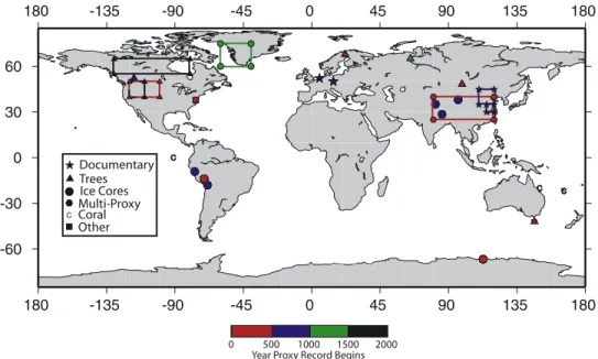
evidence, and terrestrial and ice borehole data must use less direct ‘‘spatial’’ methods of calibration. A brief discussion of the two basic approaches (temporal and spatial) to calibration is given in section 3.1. Such ‘‘coarser’’ proxies are valuable for the insight they provide into broad patterns of climate variability on longer timescales. However, attempts to reconstruct high-frequency climate patterns over the past few centuries to millennia have been restricted to annually to decadally resolved indicators, such as tree rings, corals, ice cores, lake sediments, and the few available multicentury documentary and instrumental series that are available in past centuries (Figure 1).

2.1. Instrumental Climate Data

[11] Instrumental records are by far the most reliable of all available climate data. They are precisely dated, require either no explicit calibration, or employ physically based calibrations (e.g., a mercury thermometer). These data, which include thermometer-based surface temperature measurements from the ocean and land regions, sea level pressure (SLP) measurements, continental and oceanic precipitation measurements (including drought indices), sea ice extents, and winds and humidity estimates, are, however, only available on a widespread basis back to

1850. Moreover, random, systematic, and time-varying biases may exist to some extent in all instrumental data sources [Jones et al., 1999]. Such biases include possible

residual urban warming biases in thermometer-based tem-perature measurements and under-catch issues in precipita-tion (particularly of snowfall) gauge estimates [e.g.,Folland et al., 2001a].

[12] Of primary interest from the point of view of recent global warming and past global temperature trends is the instrumental surface temperature data set. This is based on a compilation of marine (ship-based ocean sea surface tem-perature(SST) observations) and terrestrial (stationsurface air temperature (SAT) measurements) sources. Several compilations provide gridded monthly mean estimates of temperatures on a large-scale basis back through the mid-19th century [e.g.,Jones et al., 1986;Hansen and Lebedeff, 1987;Vinnikov et al., 1990;Jones and Briffa, 1992;Briffa and Jones, 1993;Wigley et al., 1997;Peterson et al., 1998;

Hansen et al., 1999, 2001; Jones et al., 1999, 2001b]. Coverage becomes increasingly sparse, however, in many parts of the world in earlier decades (see examples in Figures 2a and 2b). A number of studies have used statistical methods to infill the instrumental surface temper-ature record back through the mid-19th century [Smith et al., 1996;Kaplan et al., 1997, 1998;Folland et al., 2001a, 2001b;Rutherford et al., 2003; Rayner et al., 2003]. The statistical methods employed make use of spatial covariance information from the relatively complete (e.g., post-1950) measurements to interpolate earlier missing data. While useful from the point of view of providing globally com-Figure 1. Map of available high-resolution (annual or decadal) proxy indicators with a verifiable

temperature signal (see Figure 4) available over much of the past two millennia. The sources of all the data are given in Table 1. The boxes represent the regions of multiproxy (as opposed to single-location proxies) composite series (e.g., for the ice core composite series from Greenland).

Figure 2. Maps and time series of 5by 5grid box instrumental temperature data: (a) percent coverage of the Hadley Centre/Climatic Research Unit version 2 (HadCRUT2v) data set [Jones and Moberg, 2003] for the 1856 – 2002 period, (b) percent coverage over the 1951 – 2002 period, and (c) 20-year smoothed annual average values for the Northern Hemisphere (from HadCRUT2v [Jones and Moberg, 2003]), central Europe, Fennoscandia, and central England. The construction of these European series is detailed byJones et al.[2003c] for continental Europe and byParker et al.[1992] for central England.

plete climate fields, there are many issues to consider with respect to assumptions of stationarity of spatial climate relationships [e.g.,Schneider, 2001;Mann and Rutherford, 2002;Rutherford et al., 2003;Pauling et al., 2003].

[13] Longer instrumental SAT measurements are available on a restricted regional basis for parts of Europe and North America back to the mid-17th century [e.g., Bradley and Jones, 1993, 1995b;Jones, 2001;Camuffo and Jones, 2002;

Chenoweth, 2003; Moberg et al., 2003]. Many of the European series have been extensively homogenized in a number of recent studies (see references given byJones and Moberg[2003]). Here in Figure 2c we compare smoothed temperature estimates for the Northern Hemisphere (NH), central Europe, Fennoscandia, and central England, assess-ing whether the NH average can be extended back with regional-scale data. Not only is there limited agreement between the NH and the European regions, except on the longest of timescales, but there are also clear differences between the regions. The principal conclusion that can be drawn from Figure 2c is that NH averages clearly cannot be inferred from a single region. Despite this, tentative exten-sions of the Northern Hemisphere annual mean instrumental record have been attempted based on scaling composites of the sparse instrumental data available back to the mid-18th century against the more complete record of the mid-19th through 20th centuries [Mann et al., 2003a]. These estimates include additional early series from a few locations in eastern North America, India, and Siberia in addition to the Euro-pean data, so they provide a meaningful, though more highly uncertain, estimate of hemispheric temperature changes.

[14] Measures of the atmospheric circulation are provided by SLP estimates, which are also available, albeit on an increasingly sparse basis, back through the mid-19th cen-tury [Trenberth and Paolino, 1980; Allan et al., 1996;

Basnett and Parker, 1997]. Globally infilled reconstructions of SLP have been achieved using the same methods as those discussed above for surface temperature data [e.g., Kaplan et al., 2000]. Regional atmospheric circulation indices such as theNorth Atlantic Oscillation(NAO) index andSouthern Oscillation Index(SOI), which describe important modes of large-scale atmospheric variability, have been estimated farther back in time based on key long SLP station records. The NAO has been estimated back through the early 19th century, with prospects for instrumental extension (using station pressure data alone) back through the late 17th century [Jones et al., 2003b], while the SOI has been estimated back to the mid-19th century [Ko¨nnen et al., 1998]. A few longer SLP records are available two or more centuries back in parts of Europe [e.g.,Luterbacher et al., 2002a, 2002b, and references therein], India [Allan et al., 2002], and Japan [Ko¨nnen et al., 2003].

[15] Finally, as climate change may be altering patterns of hydroclimatic (moisture) variability during the 20th century [e.g.,Karl and Knight, 1998], it is important to consider the longer-term nature of moisture variations. Land-based pre-cipitation measurements have been amalgamated into grid-ded data sets [Hulme, 1992;Dai et al., 1997;Hulme et al., 1998] and extended to drought indices [Dai et al., 1998;

Cook et al., 1998], using gridded temperature and precip-itation databases, for all of the 20th century. Some long instrumental precipitation series in Europe, North America, and India are available back through the 18th century [Bradley and Jones, 1995b; Jones, 2001;Slonosky, 2002]. Drought indices based on station precipitation and temper-ature measurements have been extended back into the mid-19th century at some locations in the United States [Zhang et al., 2004] and Europe [Jones, 2001].

2.2. Historical Documentary Records

[16] These sources include records of frost dates, droughts, famines, the freezing of water bodies, duration of snow and sea ice cover, and phenological evidence (e.g., the dates of flowering of plants and the ranges of various species of plants). All can provide insight into past climate conditions [Wigley et al., 1981;Bradley and Jones, 1995a;

Bradley, 1999; Luterbacher et al., 2002a, 2002b]. Docu-mentary evidence is, however, generally limited to regions with long written traditions, such as Europe [e.g.,Bradley and Jones, 1995a; Le Roy Ladurie, 1971;Martin-Vide and Barriendos, 1995;Pfister et al., 1998;Rodrigo et al., 1999;

Ogilvie and Jo´nsson, 2001; Bra´zdil et al., 2004], eastern Asia [Wang and Zhao, 1981; Zhang and Crowley, 1989;

Wang et al., 2001], and, more recently, North America [Bradley and Jones, 1995a; Druckenbrod et al., 2003;

Overland and Wood, 2003]. However, logs from Spanish galleons crossing the Pacific Ocean during the 16th – 19th centuries provide possible insights into variations in the strength of the prevailing winds [Garcia et al., 2001], and documentary information from South America enables a chronology of El Nin˜o [Quinn and Neal, 1992; Ortlieb, 2000] to be developed over the past few centuries. Human accounts (e.g., through artistic depictions) of mountain glacier retreats and advances during past centuries provide evidence of climate change on more low-frequency time-scales. Some of this type of evidence is more anecdotal, and we discuss this, with examples, at the end of this section. We emphasize here issues in the development of long index series from documentary sources.

[17] Despite the wealth of data available in some regions, documentary sources alone are not useful for detailing truly global-scale climate variations and must, furthermore, be interpreted with caution, as they are not equivalent in their reliability to actual instrumental measurements of meteoro-logical variables. Historical documentary information often emphasizes extreme conditions (i.e., heat waves and cold snaps) [see, e.g.,Pfister, 1992]. This may provide a highly misleading sense of the true seasonal or annual mean climate anomalies that are of interest in the context of discussions of climate change. It has been shown [e.g.,

Thompson and Wallace, 2001] that change in the phase of the North Atlantic Oscillation/Arctic Oscillation(NAO/AO) pattern of winter atmospheric circulation variability (see section 4.4.3) can result in roughly a tripling (Orlando, Florida) to nearly a tenfold (Paris, France) increase in the incidence of cold winter temperature extremes, even in the context of far more modest changes (1or 2C) in seasonal

mean temperatures in these regions. It is likely [Shindell et al., 2003] that such atmospheric circulation changes are therefore responsible for many of the reports of extreme cold spells in Europe during the 17th – 19th centuries [e.g.,

Pfister, 1992], despite evidence indicating more moderate mean temperature changes [Mann et al., 2000a;Shindell et al., 2003].

[18] Historical documentary climate reconstructions based on combinations of information from different observers may be further biased as the qualitative standards used to reflect climate conditions are likely to be observer-dependent. Does the ‘‘wettest summer in living memory’’ have the same meaning to observers living at least a century apart? Not only is linguistic knowledge vital but so are changes in the meaning of currently used words. The word ‘‘gale’’ took on its present usage just before Francis Beau-fort developed his wind force scale (1810) used ever since by mariners. Before 1750, however, every wind above force 4 was recorded as a ‘‘gale’’ by English mariners, generally with a qualifier. The current word ‘‘breeze’’ entered the English vocabulary (probably from Catalan) during the later half of the 18th century.

[19] Development of long series therefore needs to be undertaken with care and in a consistent and repeatable way. The principal keys to developing long series of reliable climatic measures are the selective use of contemporarily reported material [Ingram et al., 1981] and rigorous assess-ment of reporters (e.g., using content analysis [Baron, 1982]). It becomes more difficult to verify the fewer records available in earlier periods. In the High Medieval Age (A.D. 1000 – 1250 [Bradley et al., 2003]), chroniclers in Europe often included reports from neighboring regions and countries, and with even small cities using different calen-dars and saints’ days, the potential for misrecording of events is rife (generally through duplication). All protago-nists (exemplified byBell and Ogilvie[1978]) of documen-tary evidence stress the need to consult the original sources and not to use late 19th or 20th century compilations (such as those ofEaston[1928] andBritton[1937]). Many highly respected climatologists pioneering the use of documentary climate histories in the 1960s [e.g., Lamb, 1965; Bryson, 1962] sometimes used less than reliable sources of infor-mation taken from such questionable compilations [see, e.g., Ogilvie and Farmer, 1997]. A most recent and very comprehensive review of the documentary data archive has been provided by Bra´zdil et al. [2004]. Useful additional discussions are given by Mikami [1999] and Jones et al.

[2003a].

[20] Historical documentary series must be considered ‘‘proxy’’ climate records as they require independent cali-bration against instrumental climate data for any reliable, quantitative interpretation in terms of, for example, seasonal/ annual temperature or precipitation/drought variations. This is often extremely difficult, and various approaches have been introduced [Pfister, 1984, 1992; van Engelen et al., 2001;Jones et al., 2003a]. It is clear that the quality of the preinstrumental part of any documentary series must be of a lesser quality than the modern instrumental part [Jones et al.,

2003a], and users should be mindful of this, particularly with respect to calibration exercises (see section 3.1), when developing multiproxy compilations.

[21] We have thus far emphasized the work of historical climatologists who have combined detailed information and rigorous statistical techniques in order to develop long, continuous, and well-replicated series. Despite these exten-sive research efforts, anecdotal evidence concerning the last millennium based on factually dubious beliefs is still rife. We note three specific examples that are often misrepre-sented in terms of their relevance to past climate: (1) the freezing of the River Thames in London in past centuries, (2) the cultivation of vines in medieval England, and (3) the settlement of Iceland and southwestern Greenland about 1000 years ago. It is not unusual to find any one of these examples (often referred to as anecdotal information), and indeed, in some cases, all three simultaneously [Cutler, 1997], incorrectly presented as evidence of large-scale warmth or cold in popular accounts of past climate change. Examples can also be found in the peer review scientific literature [Soon and Baliunas, 2003;Soon et al., 2003] (see also the discussion given byMann et al.[2003a]).

[22] 1. River Thames freeze-overs (and sometimes frost fairs) only occurred 22 times between 1408 and 1814 [Lamb, 1977] when the old London Bridge constricted flow through its multiple piers and restricted the tide with a weir. After the bridge was replaced in the 1830s, the tide came farther upstream, and freezes no longer occurred, despite a number of exceptionally cold winters. The winter of 1962/ 1963, for example, was the third coldest in the central England temperature(CET) record (the longest instrumen-tal record anywhere in the world extending back to 1659 [Manley, 1974;Parker et al., 1992]), yet the river only froze upstream of the present tidal limit at Teddington. The CET record clearly indicates that Thames (London) ‘‘frost fairs’’ provide a biased account of British climate changes (let alone larger-scale changes, see Figure 2c) in past centuries. [23] 2. Monks in medieval England grew vines as wine was required for sacramental purposes. With careful hus-bandry, vines can be grown today, and indeed, vineyards are found as far north as southern Yorkshire. There are a considerably greater number of active vineyards in England and Wales today (roughly 350) than recorded during medie-val times (52 in theDomesday Book of A.D. 1086). Vine growing persisted in England throughout the millennium. The process of making sparkling wine was developed in London (by Christopher Merret) in the 17th century, fully 30 years before it began in the Champagne region of France. Thus the oft cited example of past vine growing in England reflects little, if any, on the relative climate changes in the region since medieval times.

[24] 3. Iceland was settled mainly from Norway and the northern British Isles beginning A.D. 871. The further migration to SW Greenland approximately one century later, by a small group of Icelanders, was the result primarily of a political and economic need to leave Iceland [Ogilvie and Jo´nsson, 2001]. Climate was not a factor in their decision despite claims otherwise that still appear in

the literature [Soon and Baliunas, 2003;Soon et al., 2003]. The SW Greenland settlements survived for many centuries, but in the mid-14th century the more marginal and more northerly located Western Settlement was abandoned. There were a number of reasons for this, including culture and economic factors. However, it seems likely that climate did play a part in the abandonment. The focus of their economy on animal husbandry denied them the advantages of hunting marine and other mammals that ensured the survival of their Inuit neighbors. A series of unusually late springs and cold summers, for example, may have helped to make a marginal situation untenable [Barlow et al., 1997]. The more south-erly Eastern Settlement survived to around the mid-15th century [Buckland et al., 1996]. Related myths exist for the North American continent.Overland and Wood[2003], for example, have recently demonstrated that, despite past claims that the extreme cold of the ‘‘Little Ice Age’’ (LIA) impeded the navigation of a Northwest Passage in the Canadian Arctic during the early 19th century, an exhaus-tive study of 19th century explorer logs for the region yields no evidence of unusually cold conditions.

2.3. Tree Ring Records

[25] Tree ring or ‘‘dendroclimatic’’ proxy climate indica-tors can provide information regarding past seasonal tem-peratures or precipitation/drought, based on measurements of annual ring widths and/or maximum latewood densities [Fritts, 1976, 1991; Fritts et al., 1971; Schweingruber, 1988; Jacoby and D’Arrigo, 1989; Briffa et al., 1992a, 1992b, 1998b; Hughes and Funkhouser, 1999; Stahle et al., 1998a, 1998b; Cook et al., 1999; Briffa and Osborn, 1999, 2002;Briffa et al., 2001]. While tree ring data are the most widespread source of annually resolved proxy climate information and exhibit some of the strongest statistical relationships with instrumental climate records [Jones et al., 1998], they are limited to where trees can be cross-dated and chronologies developed. They are found in most subpolar and midlatitude terrestrial regions. Generally only extratropical species are useful for climate reconstruction, though there are some exceptions (e.g., tropical teak in Indonesia/Southeast Asia [Jacoby and D’Arrigo, 1990; see also Stahle, 1999; Stahle et al., 1999]). Tree ring recon-structions offer the advantage of potentially being quite long (e.g., several millennia) [Hughes and Graumlich, 1996;

Cook et al., 2000;Briffa and Osborn, 2002].

[26] The relative strengths and weaknesses of different ‘‘standardization’’ methods for preserving climate variabil-ity on multicentennial timescales from tree ring measure-ments derived by combining shorter length ‘‘segmeasure-ments’’ is actively discussed in the literature [Cook et al., 1995;Briffa et al., 1996;Esper et al., 2002; Briffa and Osborn, 2002;

Mann and Hughes, 2002]. Reconstructions developed in the last decade use conservative techniques such as regional curve standardization(RCS) [Briffa et al., 1992a] andage

-band decomposition(ABD) [Briffa et al., 2001] to develop series that capture more low-frequency climate variability. These approaches are now widely used but they are not applicable for all sites as large numbers of sample series are

required to maintain a similar age structure to the chronol-ogy over time [Cook et al., 1990;Mann and Hughes, 2002]. RCS and ABD approaches are unlikely to be the last word on ‘‘standardization,’’ and site selection is still very impor-tant [Fritts et al., 1971;Schweingruber, 1988]. The empha-sis on standardization underscores the importance of longer-timescale information in reconstructions. As instrumental data will always be too short to adequately address this issue, low-frequency variability should be compared, where possible, with information from other proxy sources in the region.

[27] During the most recent decades, there is evidence that the response of tree ring indicators to climate has changed, particularly at higher latitudes and more so for density than ring width measurements [Briffa et al., 1998a]. One suggested source for this behavior is ‘‘CO2 fertiliza-tion,’’ the potential enhancement of tree growth at higher ambient CO2 concentrations. Though it is extremely diffi-cult to establish this existence of this effect [Wigley et al., 1988], there is evidence that it may increase annual ring widths in high-elevation drought-stressed trees [Graybill and Idso, 1993]. Recent work making use of climate reconstructions from such trees has typically sought to remove such influences prior to use in climate reconstruc-tion [Mann et al., 1999; Mann and Jones, 2003]. Other factors have been suggested as possible explanations for apparent anomalous tree ring/climate relationships [see

Briffa et al., 1998a], including the changing seasonality of the climate itself [Vaganov et al., 1999; Biondi, 2000;

Druckenbrod et al., 2003]. The potential existence of such nonstationary relationships introduces an additional caveat in the use of tree ring data alone for climate reconstruction, since changes in environmental factors in the past could have introduced similar, unknown changes in tree ring response to climate.

[28] Carbon and oxygen isotopes from tree rings have been considered as potential climate proxies, but a straight-forward interpretation of the measurements has proven elusive [White, 1989]. While there has been some promising recent work in this area [Leavitt et al., 1995;Robertson et al., 1997; Anderson et al., 1998], tree ring isotopes have not been used in large-scale climate reconstruction. Intertree variability needs to be assessed for isotopic measurements. Isotopic analyses require considerably greater effort than traditional tree ring analyses based on ring width and density measurements. As this added effort should be cost-effective relative to the usefulness of the results, it still needs to be demonstrated that fewer numbers of individual cores/trees need be isotopically analyzed to obtain an equivalent climate signal, when simpler methods are available.

2.4. Coral Records

[29] Corals can also provide useful proxy climate infor-mation (see Dunbar and Cole[1999] for a review). Proxy reconstructions from corals generally rely on geochemical characteristics of the coral skeleton such as temporal varia-tions in trace elements (e.g., Sr/Ca chemical ratios) or stable isotopes (e.g., oxygen isotopes) or, sometimes, on density or

variations in fluorescence [e.g., Isdale et al., 1998] of the coral’s aragonite structure. Because they offer information regarding tropical and subtropical maritime regions, corals are complementary in terms of the spatial climate informa-tion provided by tree ring data. Corals can be precisely (annually or even seasonally) dated and their environment can be continuously sampled over the full year, providing a potentially more uniform window of climatic information than other more seasonally specific proxies. Because of their potential to sample climate variations in ENSO-sensi-tive regions [e.g.,Cole et al., 1993;Dunbar et al., 1994], a modest network of high-quality coral site records can resolve key patterns of tropical climate variability [Evans et al., 1998, 2002]. However, though recent work has shown some promise in moving toward the possibility of millennial-length reconstructions based on the combination of overlapping multidecadal and century-length fossil corals [Cobb, 2002], very long, multicentury records are rare. The longest continuous coral series extend back to the early 16th century [see Dunbar and Cole, 1999], but ‘‘snap-shots’’ of 50 – 150 years in duration have been used to assess ENSO variability during the past millennium [Cobb, 2002;Cobb et al., 2003a] and various other intervals for the whole Holocene [e.g.,Tudhope et al., 2001, and references therein]. Such an approach has important limitations. A fossil coral must be growing at similar depths to its modern counterparts (specifically those corals used to calibrate against the instrumental record), and any inferred climate changes must be measured against the ability of individual modern corals at that site to accurately reflect 20th century climate changes. Diagenetic alterations in fossil corals can be extremely difficult to detect and could significantly bias fossil coral-based estimates of past climate change. Given these limitations, the most useful estimates come from multiple fossil coral ‘‘snapshots’’ from a given time period. [30] While corals have demonstrated an excellent ability to describe climate variability on interannual and decadal timescales [Cole et al., 1992, 1993, 1995; Dunbar et al., 1994, 1996;Slowey and Crowley, 1995; Wellington et al., 1996;Quinn et al., 1996, 1998;Crowley et al., 1997, 1999;

Lough and Barnes, 1997;Felis et al., 2000;Linsley et al., 2000;Cobb et al., 2001;Hendy et al., 2002], their reliability on longer timescales has not been adequately established. The effects of temperature and salinity (through ocean water oxygen isotopic composition) involve potentially competing and even conflicting influences on coral oxygen isotopic composition. Estimates of low-frequency variability or long-term changes [e.g., Winter et al., 2000] based on calibration of oxygen isotope ratios against instrumental data that are short (a few decades) and/or dominated by a seasonal cycle (and therefore may reflect a balance of salinity and temperature influences only appropriate to that timescale) are therefore unlikely to yield reliable recon-structions of the variable (e.g., SST) of interest [Crowley et al., 1999; Juillet-Leclerc and Schmidt, 2001]. Possible influences of ‘‘vital effects’’ (e.g., nonclimatic influences on the coral’s biochemistry) may effect the reliability of climate reconstructions based on single specimens [e.g.,

Cardinal et al., 2001]. Despite these limitations, recent work [e.g.,Correge et al., 2001;Quinn and Sampson, 2002;Hendy et al., 2002] has pioneered the use of multiple measurements (e.g., Sr/Ca and oxygen isotope ratios) from the same coral to simultaneously estimate SST and salinity influences, and coral paleoclimatology, while still in its early stages, shows considerable promise [see, e.g.,Evans et al., 2002].

2.5. Ice Core Records

[31] Ice cores provide climate information over multiple millennia from the polar regions of both the Northern [e.g.,

O’Brien et al., 1995; Fisher et al., 1996; Appenzeller et al., 1998;White et al., 1997;Hoffman et al., 2001;Moore et al., 2002; Vinther et al., 2003] and Southern [Peel et al., 1996; Mayewski and Goodwin, 1997; Morgan and van Ommen, 1997] Hemispheres, as well as alpine (tropical and subtropical) environments [Thompson, 1992, 1996;

Thompson et al., 2000, 2003]. Ice core information is thus spatially complimentary to that provided by either tree rings or corals, but it is available only over a very small fraction of the global surface. Ice cores can provide several climate-related indicators, including the fraction of melting ice, the rate of accumulation of precipitation, and concentrations of various chemical constituents (including trace gases) that provide information about the atmospheric environment [e.g., O’Brien et al., 1995; Meeker and Mayewski, 2002] at the time the ice was deposited. Ice cores also contain cosmogenic isotopes of beryllium and volcanic dust, both providing sources of vital information regarding the past radiative forcing of climate (see section 5).

[32] Of primary use from the point of view of climate reconstruction, however, are stable isotopes of oxygen (and, in some cases, deuterium) recorded in ice cores, which can, in principle, be related to temperature-dependent fraction-ation processes. To the extent that fractionfraction-ation dominates at the time of deposition, the oxygen isotope ratios can be related to local temperature conditions, providing a ‘‘paleo-thermometer.’’ However, the added influence of nonlocal fractionation on the isotopic ratios measured by a given ice core means that in practice a simple ‘‘paleothermometer’’ calibration remains elusive [Hoffman et al., 1998]. Annual dating is possible in principle, but in practice it is often quite difficult, and generally, the dating is not precise. Use of stratigraphic markers (like known volcanic dust events), where available, can help anchor the age model [e.g.,

Clausen et al., 1995]. Stacking of multiple annual-timescale ice core records [e.g., Fisher et al., 1996; Vinther et al., 2003] can reduce the age model uncertainty in chronologies and reduce between-site variability. In regions with low snowfall, 1 year’s accumulation may represent a small number of discrete precipitation events. In such cases, annual dating may not be possible, and there is furthermore the potential for a substantial temporal (and seasonal) sampling bias. In regions where accumulation is high (e.g., Law Dome, Antarctica) or where a number of cores can be cross-dated like trees (e.g., Greenland), seasonal resolution is possible. Here well-dated proxy estimates of millennial or greater length are possible [van Ommen and

Morgan, 1996, 1997; Fisher et al., 1996; Vinther et al., 2003].

2.6. Speleothems

[33] Speleothems (cave deposits) are formed as a part of the meteoric water cycle, and variations in their growth rates and composition reflect environmental changes on the land surface above the cave [Lauritzen and Lundberg, 1999, and references therein]. Various proxies have been studied, including growth rates, isotopic composition, trace elements, organic matter content, and luminescent laminae. Locations are limited, but studies have been undertaken at a number of sites in North America, Eurasia, the tropics, southern Africa, and Australasia. Without replication, uncertainties associated with dating the speleothem (gener-ally by laminae counting and uranium series methods) are an issue despite apparent annual resolution at many sites. Interpretation of the possible proxies is also difficult in terms of a simple climate variable (e.g., temperature) because of the multiple potential influences (e.g., source temperature, seasonal changes in rainfall, groundwater residence time, etc.) on the speleothem’s geochemistry and/or morphology [see Bradley, 1999]. Despite difficulties in interpreting speleothem records they can often provide information about changes in the hydrological cycle and through this links to the atmospheric circulation [McDermott et al., 1999;Proctor et al., 2000;Frappier et al., 2002] and even past cultural changes [Polyak and Asmerom, 2001].

2.7. Varved Lake and Ocean Sediment Records

[34] Annually laminated (varved) lake sediments, like ice cores, provide high-resolution proxy climate information in high-latitude regions where other proxy indicators, such as tree rings, are not available [Lamoureux and Bradley, 1996;

Hardy et al., 1996;Overpeck et al., 1997;Wohlfarth et al., 1998;Hughen et al., 2001]. Varved sediments formed from the deposition of inorganic sediments (clastic) are controlled by seasonal precipitation and summer temperature, both of which govern the volume of meltwater discharge and sediment load into a closed-basin glacial lake. When the latter process dominates the deposition process, the annual (or even subannual) varve thicknesses provide inferences into summer temperature variations [e.g., Overpeck et al., 1997;Hughen et al., 2001]. In rare cases, annually varved [Hughen et al., 1996;Biondi et al., 1997;Black et al., 1999] sediments can be obtained from marine (coastal or estua-rine) environments where deposition is unusually high, and proxy climate information can be obtained from oxygen isotopes or faunal assemblages contained within the sedi-ments. If adequate radiometric dating is available (e.g., through pollen biostratigraphy), nonvarved lake [e.g.,Laird et al., 1996, 1998;Moy et al., 2002] and estuarine [Cronin et al., 2003] sediments can still provide useful climate information at decadal timescales in past centuries.

2.8. Boreholes

[35] Boreholes can provide estimates of past temperature variability, though their resolution is intrinsically multi-decadal at its finest and decreases back in time.

Borehole-derived temperature estimates come from two distinct sources: widespread terrestrial boreholes in tropical, mid-latitude, and subpolar environments [e.g., Beltrami et al., 1995; Harris and Chapman, 1997, 2001; Pollack et al., 1998; Huang et al., 2000; Mann et al., 2003b] and ice boreholes from polar ice caps [e.g., Dahl-Jensen et al., 1998]. In both cases the subsurface borehole temperature profiles are used to obtain an estimate of ground (or ice)

surface temperature (GST) changes back in time through solution of an appropriate inverse problem. This is generally achieved by inverting the diffusion equation [e.g.,Shen and Beck, 1991] that describes the downward propagation of surface temperatures into the ground and requires some a priori knowledge and several assumptions. These include the homogeneity of the medium and absence of advective heat transport by fluid flow [see Shen et al., 1995], the thermal properties of the medium, and the nature of the background geothermal heat flux that must be removed to yield an estimate of transient surface-forced temperature variability [seeHarris and Chapman, 1997;Pollack et al., 1998;Huang et al., 2000;Harris and Chapman, 2001].

[36] While borehole temperature profiles, in principle, provide a direct measurement of GST histories, GST potentially differs in some fundamentally important ways from the quantity, surface air temperature (SAT), which is typically of interest in discussions of large-scale climate variability. GST is impacted by changes in seasonal snow cover [e.g.,Zhang et al., 2003;Mann and Schmidt, 2003;

Stieglitz et al., 2003; Beltrami and Kellman, 2003], land surface changes [e.g.,Skinner and Majorowicz, 1999], and various other potential factors (often seasonally specific) unrelated to SAT changes. These complicate interpretation of GST estimates in terms of past changes in overlying SAT [Folland et al., 2001a; Mann et al., 2003b; Mann and Schmidt, 2003;Beltrami and Kellman, 2003]. The existence of a cold season bias has now been demonstrated in two climate model simulations [Mann and Schmidt, 2003;

Gonzalez-Rouco et al., 2003], but the implications for past annual mean temperature changes are unclear [ Gonzalez-Rouco et al., 2003]. These depend on the actual history of cold season snow cover changes in past centuries, which cannot be recovered in any single model simulation. An additional consideration is the restricted and spatially var-iable sampling of past GST variations provided by available global borehole networks [Pollack et al., 1998; Huang et al., 2000], which may yield a biased estimate of large-scale mean temperature change [Briffa and Osborn, 2002;Mann et al., 2003b]. Despite the various possible sources of bias in estimating large-scale SAT trends in past centuries from borehole data, the apparent discrepancies with other proxy-based estimates appear to be diminished when an attempt is made to account for spatial sampling biases [Briffa and Osborn, 2002; Mann et al., 2003b] and when an optimal estimate is made via spatial regression [Mann et al., 2003b;

Rutherford and Mann, 2004] of the actual SAT signal contained within the borehole GST estimates (Figure 3).

[37] Ice borehole records are less likely to suffer from many of these sources of bias, but a number of assumptions

when inverting the borehole profile to obtain an estimate of past ice surface temperatures, such as the presence of ice flow over time, will introduce potential chronological error into the record. They provide valuable estimates of past temperature changes in polar environments that are com-plementary to those obtained from ice core oxygen isotopes [Dahl-Jensen et al., 1998]. Significant differences between ice borehole temperature estimates obtained at relatively nearby sites (Dye3 and Greenland Ice Core Project [see

Dahl-Jensen et al., 1998]) suggest that the contribution of local noise or possible biases in isotope records may be substantial. Inferences with regard to past temperature changes from the two locations should be interpreted with appropriate caveats. They are sufficiently reliable, however, to indicate that temporal calibration techniques must be applied to ice core isotopic measurements. Use of the seasonal cycle or spatial variations in isotopic ratios to determine a temperature scale cannot be objectively justi-fied (see also section 3.1).

2.9. Glacial Evidence

[38] The position of glacial moraines (till left behind by receding glaciers) can provide information on the advances (and, less accurately, the retreats) of mountain glaciers in past centuries. This can be interpreted, at least indirectly, as past changes in regional glacial mass balance, which reflect (though in a relatively complex way) past climate variations [e.g., Grove and Switsur, 1994]. Simple interpretation of such information in terms of past surface air temperature and precipitation changes is, however, confounded by the delicate balance between local changes in melting and ice accumulation and the variable response timescale of glacial mass balance (which typically increases with the size of the glacier, potentially approaching century timescales for large mountain glaciers). In other words, glacial moraine evi-dence may be indicative of past climate variability, but it

cannot, despite claims sometimes made to the contrary [e.g.,

Broecker, 2001], be uniquely interpreted in terms of specific past temperature or precipitation histories. Both increased winter precipitation (through greater accumulation) and lower summer temperatures (through decreased melting or ‘‘ablation’’) can lead to more positive glacial mass balances. While the response to climate forcing may be close to contemporaneous for small, fast moving glaciers, the inertia of large glaciers dictates that they respond to climate change relatively slowly, with delays of decades or occasionally centuries [Jo¨hanneson et al., 1989]. A more promising approach to making use of glacial moraine evidence for paleoclimatic interpretation involves the use of forward modeling in which the history of past glacial mass balance is compared to the evolution of a glacial mass balance model using reconstructions from high-frequency proxy indicators (e.g., many tree-based summer temperature reconstructions) or possibly climate model estimates of past and future temperature and precipitation scenarios as boundary conditions [Oerlemans, 1992;Raper et al., 1996;

Folland et al., 2001a;Reichert et al., 2002].

2.10. Other Proxy Records

[39] Other possible high-resolution proxy indicators are potentially useful but as yet are still under development in terms of their use in climate reconstruction. These include isotopes from molluscs [Weidman and Jones, 1994]. In some shallow seas of the North Atlantic region it should prove possible (but with considerable effort) to develop annual-timescale chronologies for the late Holocene based on the clam,Arctica Islandica.

[40] In addition, lower-resolution indicators that are dif-ficult to calibrate against instrumental records can, none-theless, sometimes assist our understanding of long-term climate variability from at least a qualitative point of view. For example, open ocean sedimentation rates may some-Figure 3. Estimates of Northern Hemisphere mean surface temperature changes over the past five

centuries from terrestrial borehole data are shown, based on a simple (unweighted) arithmetic average of available borehole data [Huang et al., 2000], an areally weighted average of the borehole data, and a statistically optimal hemispheric surface temperature estimate (and its 2 standard error uncertainties, shaded region) from the available borehole data [Mann et al., 2003b]. Shown for comparison is the instrumental record of Northern Hemisphere temperature through the mid-19th century (based on HadCRUT2v [Jones and Moberg, 2003]) and an extension back through the mid-18th century based on sparser instrumental data [Mann et al., 2003b]. The areally weighted and ‘‘optimal’’ borehole estimates are revised relative toMann et al.[2003b] based on the correction of an error in the normalization of the areal weighting that has been identified in the original analysis [Rutherford and Mann, 2004].

times be sufficiently high that century-scale or at least multicentury variability can be resolved, even if annual ‘‘varves’’ or other means of high-resolution dating are not available [e.g.,Keigwin, 1996;Keigwin and Pickart, 1999;

Anderson et al., 2002]. In such cases, however, any quan-titative reconstructions of climate variables based on the use of ‘‘paleothermometer’’ calibration approaches (e.g., the ‘‘spatial’’ approach, see section 3.1 and discussion in sections 2.4 and 2.5) are potentially unreliable. Also, in many cases, age determination relies on radiometric meth-ods with relatively poor age control, and uncertainties may be of the order of a century or more. Quantitative estimates of past climate variability from sediment cores should thus be interpreted with caution. Similar arguments hold for any low-resolution reconstructions (sediment cores or pollen data) for which an a priori (e.g., paleothermometer or spatial transfer function) rather than an explicit (i.e., correlation against instrumental data) calibration technique is used to establish a quantitative scale for the variable of interest [see, e.g., Bradley, 1999].

[41] One of the most widespread low-temporal-resolu-tion proxies is past pollen records from cores taken on land or from lakes (see European summary by Huntley and Prentice[1993]). Inferences about the climate can be made on timescales of 500-1000 years, but, as with varved sediments, they are subject to dating uncertainties. The vegetation composition of a region takes some time to respond to climate change, so interpretation can be com-plicated by both response time issues and uncertainty in the nature of the underlying climate signal. Faunal remains (e.g., beetles and chironomids) offer the advantage of a contemporaneous response to underlying climate changes but are subject to similar dating uncertainties as pollen [Atkinson et al., 1987]. Another low-resolution indication of past climate is provided by earlier tree line positions (see

Shiyatov [1993] but see also Nichols [1975]). Climatic inferences here might be specific to short periods when trees were able to survive beyond the sapling stage at higher elevations than present. Once established, trees can survive for many hundreds of years, so that indications of warmer conditions may only be representative of those during their early years of life.

3. PROXY CLIMATE RECONSTRUCTIONS

3.1. Calibration of Proxy Data

[42] There are two basic approaches to the calibration of proxies against instrumental climate data. Both are based on linear regression methods but can be distinguished by their use of temporal or spatial relationships. With the temporal approach the strength of the climate ‘‘signal’’ in the proxy is assessed by time series regression against instrumental climate data. Much of the terminology used comes from the field of dendroclimatology, for which there is a long tradition of the development and application of rigorous statistical methods [e.g., Fritts et al., 1971; Fritts, 1991;

Cook and Briffa, 1990]. The first step in the regression process is to assess which part of the year or season the

proxy responds to. The quantitative relationship between the proxy and seasonal/annual instrumental data is then determined for a ‘‘calibration’’ period with some instrumen-tal data withheld to assess the veracity of the relationship with independent data (the ‘‘verification’’ period) [Briffa, 1995]. If statistical measures are considered adequate, the principle of uniformitarianism [e.g., Bradley, 1999] is invoked to reconstruct the climate series from the earlier variability of the proxy.

[43] In the spatial approach (exemplified in palynology) the quality of the proxy climatic signal is determined by assemblages of the proxy (e.g., pollen) in today’s climate from a number of locations. A spatial transfer function [e.g., Berglund et al., 1996] is then developed that takes assemblages in earlier times to infer past climate. A slight alternate to this has often been used in ice cores and corals. In this, isotopic ratios (e.g., d18O or dD) are regarded as direct measures of temperature with the constants of proportionality determined by the spatial variability of the isotopic ratios and temperature. Time series calibration appears superior, however, to the use of spatial/geograph-ical variations. The latter approach has been shown to be unreliable with respect to isotope/temperature relationships (e.g., the reassessments in polar ice cores with borehole approaches [Dahl-Jensen et al., 1998]) and in the case of corals with respect to calibration using the seasonal cycle [Crowley et al., 1999].

[44] The use of instrumental climate data records is an essential component of high-resolution paleoclimatology, as it provides the quantitative information against which proxy climatic indicators must be calibrated. The longer the instrumental record in the vicinity of the proxy site, the greater the potential for accurate assessment of the fidelity of a proxy reconstruction achieved by local calibration approaches. This holds true particularly with respect to assessments of the stationarity and timescale of response [Jones et al., 1998]. Calibration against local instrumental data is clearly much more of a challenge in data-sparse regions such as the Antarctic and the continental interiors of South America and Africa. Some recent progress has been made in the blending of modern satellite and in situ surface temperature measurements in Antarctica [Schneider and Steig, 2002], which should prove useful for the calibration of Antarctic ice core data [Steig and Schneider, 2002].

[45] For all annually resolved proxy data (sections 2.2 – 2.7) the temporal approach provides the most reliable measures of potential proxy performance in the preinstru-mental period. Here we reassess all the temperature proxy series we use (those displayed in Figure 4) by comparing the series with instrumental data. The results are given in Table 1. Correlations are calculated for the 1901 – 1980 period at both the annual and decadal timescale (for annu-ally resolved series) and just the decadal timescale for less well resolved series. The upper limit of 1980 was chosen because many of the proxy series are not available for the most recent decades, while the lower limit of 1901 was chosen because of the increasing sparseness of the

instru-mental record prior to the 20th century. For the majority of series we compare with instrumental calendar year average temperatures (based on individual or multiple 5by 5grid boxes from the Hadley Centre/Climatic Research Unit version 2 (HadCRUT2v) data set of Jones and Moberg

[2003]). For some higher-latitude NH tree-based reconstruc-tions we use a more appropriate ‘‘growing season’’ of May to September. Southern Hemisphere series might be im-proved slightly with a possibly more relevant ‘‘year’’ such as July to June. However, for consistency of comparison we have considered just the two seasonal response windows (principally, for reference to the hemispheric and global

composite series and their components, discussed with Figures 5 and 4, respectively). All correlations (with the exception of the Galapagos Islands coral) improve at the decadal timescales, although for some the increase is small and the significance less when the reduced number of degrees of freedom is allowed for. A number of other temperature reconstructions used in earlier multiproxy com-posites or in review papers [e.g.,Jones et al., 1998;Mann et al., 1998a, 1999;Mann and Jones, 2003] are not included. This is because they are either less resolved than decadal resolution [e.g., Dahl-Jensen et al., 1998] or correlations with local grid box temperatures are not significant [e.g., Figure 4. Local and regional proxy temperature reconstructions by continent. Source references for all

series are given in Table 1. Each series has been normalized over the period 1751 – 1950 and then smoothed with a 50-year Gaussian filter. For the decadally resolved data the normalization period is the 20 decades from 1750 to 1949, smoothed using a 5-decade filter.

Villalba, 1990;Lara and Villalba, 1993;Cook et al., 2002b] for the two seasonal response windows used.

3.2. Climate Field Reconstruction Approaches

[46] While individual proxy records can be calibrated against local climate data through the methods discussed in section 3.1, it is sometimes more effective to reconstruct entire (regional, hemispheric, or near global) climate fields through multivariate statistical orclimate field reconstruc-tion(CFR) approaches. Such approaches have been widely used in applications that infill missing data in instrumental climate fields [Reynolds and Smith, 1994; Smith et al., 1996; Basnett and Parker, 1997; Kaplan et al., 1997, 1998, 2000;Schneider, 2001;Mann and Rutherford, 2002; Rutherford et al., 2003; Rayner et al., 2003], but

related statistical approaches also have a long history in paleoclimate field reconstruction applications [Fritts et al., 1971; Fritts, 1976, 1991; Kutzbach and Guetter, 1980;

Guiot, 1985, 1988; Briffa et al., 1986;Cook et al., 1994;

Mann et al., 1998a, 1998b, 1999, 2000a, 2000b; Mann and Rutherford, 2002; Luterbacher et al., 2002b;Evans et al., 2002; Pauling et al., 2003; Zhang et al., 2004;

Rutherford et al., 2004].

[47] In the paleoclimatic context, CFR seeks to recon-struct a large-scale field, such as surface temperature [e.g.,

Mann et al., 1998a, 1998b;Evans et al., 1998, 2002;Zorita et al., 2003; Pauling et al., 2003], sea level pressure [Luterbacher et al., 2002b], or continental drought [Zhang et al., 2004]. CFR uses a spatial network of proxy indicators (either of the same type or a ‘‘multiproxy’’ set consisting of Figure 4. (continued)

Figure 5. Reconstructions of (a) Northern Hemisphere (NH), (b) Southern Hemisphere (SH), and (c) global mean (GLB) annual temperatures over the past one to two millennia. The expansion in Figure 5a compares a number of different NH estimates over the past 1000 years, while the main plot shows the proxy reconstructions back to A.D. 200 ofMann and Jones[2003], updated through 1995 as described in the text. Smoothed (40-year low-passed) versions of these series are shown to highlight the low-frequency variations. We avoid an ad hoc smoothing approach [e.g., Soon et al., 2004] by employing, as in the work ofMann and Jones[2003], objectively determined boundary constraints. We make use in each case of the boundary constraint among the three lowest-order constraints [Park, 1992] that minimizes the mean square error between the smoothed and raw data [seeGhil et al., 2002;Mann, 2004]. The instrumental NH [Jones et al., 1999], SH, and GLB series (red) through A.D. 2003, smoothed in this manner, are shown for comparison. Shown also (yellow shading) is the 95% confidence interval in the reconstruction (i.e., the positive and negative 2 standard error limits of the smoothed reconstructions). The various other (smoothed) NH reconstructions shown in the enlargement to Figure 5a have been scaled by linear regression against the smoothed instrumental NH series over the common interval 1856 – 1980, with the exception of the ‘‘Briffa et al.’’ series, which has been scaled over the shorter 1856 – 1940 interval owing to a decline in temperature response in the underlying data discussed elsewhere [Briffa et al., 1998a]. TheCrowley and Lowery[2000] series shown here replaces an incorrect version of the series shown in similar previous comparisons [e.g.,Mann et al., 2003a]. TABLE 1. Correlations Between Proxy Series and Local Instrumental Dataa

Location/Site Proxy Type Reference

Annual Correlation (r) (1901 – 1980) Decadal rb (1901 – 1980) Trees

Tornetrask density/widths Briffa et al.[1992a] 0.18c 0.54c

Polar Urals density/widths Briffa et al.[1995] 0.78c _0.85c

Mongolia widths D’Arrigo et al.[2001] 0.25 0.40

Northern tree line widths Jacoby and D’Arrigo[1989] 0.36d _0.71d

Western United States widths (PC) Mann et al.[1998a] 0.20 0.61

Western United States density Briffa et al.[1992b] 0.64c 0.66c

Jasper density/widths Luckman et al.[1997] 0.44c _0.49c

Tasmania widths Cook et al.[2000] 0.58 0.79

Corals

Great Barrier Reef growth layers Lough and Barnes[1997] 0.18d 0.47d

Galapagos isotopes Dunbar et al.[1994] 0.46d _0.12d

New Caledonia isotopes Quinn et al.[1998] 0.28d 0.51d

Ice cores

Greenland isotopes (six-site average) Fisher et al.[1996] 0.58 0.75

Greenland isotopes (seven-site average) Vinther et al.[2003] 0.57d 0.78d

Law Dome isotopes T. D. van Ommen et al.

(personal communication, 2003)

0.46d 0.76d

Quelccaya isotopes Thompson et al.[2003] – 0.70

Sajama isotopes Thompson et al.[2003] – 0.21

Huascaran isotopes Thompson et al.[2003] – 0.80

Guliya isotopes Thompson et al.[2003] – 0.45

Dunde isotopes Thompson et al.[2003] – 0.32

Dasuopu isotopes Thompson et al.[2003] – 0.55

Documentary

Low Countries historical sources van Engelen et al.[2001] 0.73 0.83

Czech Republic historical sources Bra´zdil[1996] – 0.94

East China historical sources Wang et al.[2001] – 0.50

North China historical sources Wang et al.[2001] – 0.52

Chinae _{mixture Yang et al.[2002] 0.17 0.22}

Shells

Chesapeake Bay shells Cronin et al.[2003] – 0.32

a

Calendar year averages are given except where stated, with italicized values not significant at the 5% confidence level. All series with the exception of China are plotted in Figure 4. Locations can also be seen in Figure 1. Instrumental data are either for the overlying 5by 5grid box (for single-site proxies) or averages of several boxes (for regional or multiproxy series) shown in Figure 1. Generally, for single-site proxies, more than one individual grid box temperature series is used to enable the instrumental series to be both longer and complete.

b

Decadal correlations are based directly on either decadally resolved proxies or on decadal filtering (Gaussian with 13 terms) of annually resolved proxies.

c

Value is for May to September season.

d

Correlation is based on <80 years, because proxy series ends before 1980 or instrumental records are not available in the early 20th century. Number of years is always >65 years, except for Law Dome when it is 24.

e

different types of proxy data), performing a multivariate calibration of the large-scale information in the proxy data network against the available instrumental data. As in the simple time series calibration approach described in section 3.1, verification of the skill of the reconstruction through ‘‘cross validation’’ against independent instrumen-tal data is essential [e.g., Cook et al., 1994; Mann et al., 1998a;Luterbacher et al., 2002b]. While various methods for accomplishing such a multivariate calibration exist, most involve the use of empirical eigenvectors of the instrumental data, the proxy data, or both [Fritts et al., 1971; Guiot, 1985, 1988;Briffa et al., 1986;Cook et al., 1994;Mann et al., 1998a, 1999, 2000a, 2000b; Evans et al., 2002].

Because the large-scale field is simultaneously calibrated against the full information in the network, there is no a priori local relationship assumed between proxy indicator and climatic variable. All indicators should, however, have been shown to respond to some aspect of local climate during part of the year.

[48] CFR uses a larger number of indicators (including both ‘‘original’’ proxy series and/or large-scale estimates already expressed as temperature anomalies by earlier local/ regional-scale calibration) in the reconstruction of a partic-ular climate field (e.g., surface temperature) compared to the ‘‘local calibration’’ approach described in section 3.1. For example, an indicator of convection/rainfall in the central Figure 5