Streaming Simplification of Tetrahedral Meshes
Huy T. Vo, Steven P. Callahan, Peter Lindstrom, Valerio Pascucci, and Cláudio T. SilvaAbstract— Unstructured tetrahedral meshes are com-monly used in scientific computing to represent scalar, vector, and tensor fields in three dimensions. Visualization of these meshes can be difficult to perform interactively due to their size and complexity. By reducing the size of the data, we can accomplish real-time visualization necessary for scientific analysis. We propose a two-step approach for streaming simplification of large tetrahedral meshes. Our algorithm arranges the data on disk in a streaming, I/O-efficient format that allows coherent access to the tetrahedral cells. A quadric-based simplification is sequentially performed on small portions of the mesh in-core. Our output is a coherent streaming mesh, which fa-cilitates future processing. Our technique is fast, produces high quality approximations, and operates out-of-core to process meshes too large for main memory.
Index Terms— Computational geometry and object modeling, out-of-core algorithms, mesh simplification, large meshes, tetrahedral meshes
I. INTRODUCTION
S
IMPLIFICATION techniques have been a major focus of research for the past decade due to the increasing size and complexity of geometric data. Scien-tific simulations and measurements from fluid dynamics and partial differential equation solvers have produced data sets that are too large to visualize with current hardware. Thus, approximations are necessary to achieve a level of interactivity that is necessary for proper analysis.Although significant work has been done in simpli-fying triangle meshes, relatively little has been done with tetrahedral meshes. Most of the work in tetrahedral simplification falls into two categories: Edge-collapse methods and point sampling methods. These algorithms assume that the entire mesh can be loaded into main memory. However, due to the high memory overhead of storing the mesh connectivity in addition to the geometry, there are limitations on the size of the data set that can be simplified in this manner.
We present an algorithm that streams the data from disk through memory and performs the simplification H. Vo, S. Callahan, and C. Silva are with the Scientific Computing and Imaging Institute, University of Utah. P. Lindstrom and V. Pascucci are with Lawrence Livermore National Laboratory.
on a localized portion of the entire mesh. Our approach consists of two steps. First, the tetrahedral mesh is arranged in a streaming format that supports coherent sequential access. Then, this streaming mesh is sequen-tially simplified using a quadric error-based scheme that respects boundaries and fields in the mesh. The resulting mesh is output in the same streaming format and can be used directly in subsequent processing.
Our streaming algorithm requires only one pass to simplify the entire mesh. Thus, the layout of the mesh is of great importance to produce high quality results. We perform an out-of-core ordering of the tetrahedral cells and store them on disk using a streaming tetrahedral mesh format. This format provides concurrent access to coherently ordered vertices and tetrahedra. It also minimizes the duration that a vertex remains in-core, which limits the memory footprint of the simplification. Our tetrahedral simplification incrementally works on overlapping portions of the mesh in-core. We use the quadric-error metric to perform a series of edge collapses until a target decimation is reached. By weighting the boundaries and incorporating the field data in our error metric, we can keep the error in the simplified approx-imation low. This results in a simplification algorithm that can efficiently simplify extremely large data sets. In addition, through the use of carefully optimized algo-rithms, linear solvers, and data structures we show that significant improvements in speed and stability can be achieved over previous techniques.
The main contributions of this paper include:
• We provide a streaming representation of tetrahedral meshes that supports coherent sequential access to the mesh elements.
• We describe a quadric-based edge-collapse simpli-fication algorithm that operates on portions of the streaming tetrahedral mesh. This operation occurs in a single pass, runs quickly, handles data of arbitrary size, respects field data, and works out-of-core.
• We improve upon previous stream simplification methods by ensuring that the output stream is co-herent in order to accommodate further downstream processing. We also introduce optimizations in the data structures and simplification algorithm which dramatically improve the speed and efficiency of
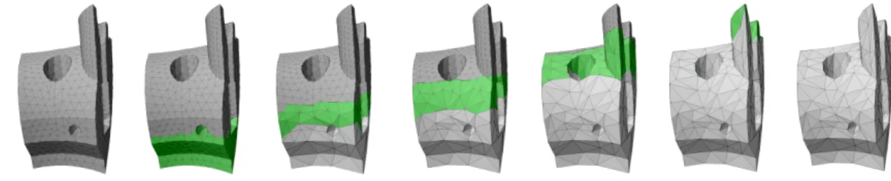
Fig. 1. Streaming simplification performed on a tetrahedral mesh ordered from bottom to top. The portion of the mesh that is in-core at each step is shown in green.
tetrahedral simplification.
• We provide a new solver for quadric-based simplifi-cation that improves stability and speed of existing algorithms. We also provide both stability and error analysis of the results generated using this tech-nique.
• We show that our streaming algorithm can suc-cessfully simplify a data set consisting of over one billion tetrahedra on a commodity PC with negligible error.
The remainder of this paper is organized as follows. We summarize related work in Section I-A. In Sec-tion II, we describe our algorithm for arranging the data in a coherent, streaming mesh. Section III provides details on our out-of-core simplification, Section IV contains our stability and error analysis followed by performance measures, Section V discusses the benefits of our approach over previous algorithms, and Section VI provides final remarks and directions for future work.
A. Related Work
A common result from scientific computations is a scalar field f inR3. This scalar field f can be represented
over a domain D as a tetrahedral mesh. When it is not possible to achieve interactive visualization of f, it is common to find a tetrahedral mesh with fewer elements and an associated scalar field f0 such that the approximation error kf0−fk is minimized. Many algorithms have been proposed in an attempt to compute
f0 quickly and with little error.
Trotts et al. [1], [2] developed a technique that collapses one edge at a time, deciding which edge to collapse next based on an error bound calculated at each step. They provide a bound on the maximum deviation of the field data in the simplified mesh from the original. Several techniques for simplification have recently been proposed that act on the vertices. Van Gelder et al. [3] remove vertices based on mass and data error metrics. Uesu et al. [4] provide a fast point-based method which works directly on the underlying scalar
field. These techniques are more memory efficient than edge collapse methods, but require the addition of Steiner points to handle non-convex meshes. This requirement makes them difficult to modify for streaming algorithms. The idea of a progressive mesh for surface level of detail control was proposed by Hoppe [5] and later extended to simplicial complexes by Popovi´c and Hoppe [6]. Staadt and Gross [7] define appropriate cost functions to account for volume preservation, gradient estimation, and scalar data with progressive tetrahedral meshes. Chopra and Meyer [8] propose a fast progressive mesh decimation scheme that is based on the scalar field of the mesh.
Many algorithms have been developed that use differ-ent error metrics to perform the simplification via edge collapses. Cignoni et al. [9] use domain and field (i.e., range) error metrics to approximate the original mesh. The use of a quadric error metric for surface simpli-fication was introduced by Garland and Heckbert [10]. Their method uses iterative contractions on vertex pairs and calculates the error approximations using quadric matrices. Natarajan and Edelsbrunner [11] extend the quadric error metric to preserve topological features. Garland and Zhou [12] recently generalized the quadric error metric for simplifying simplicial elements in any dimension.
As model size has continued to increase faster than main memory size in commodity PCs, techniques have been developed to simplify these data sets out-of-core. Lindstrom [13] proposed an algorithm that simplifies triangle meshes of arbitrary size. This algorithm im-proves upon Rossignac and Borel’s [14] vertex-clustering method by using the quadric error metric. The mesh is stored as a redundant list of three vertex positions per triangle. This “triangle soup” is read one triangle at a time and a simplified mesh is constructed incrementally and kept in-core. Lindstrom and Silva [15] improve upon the quality of this algorithm while making the method more memory efficient by storing the simplified mesh out-of-core during processing. They handle boundaries separately to preserve the overall shape of the mesh.
Wu and Kobbelt [16] propose an edge collapse-based streaming method for large triangle meshes that requires only one pass to decimate the entire mesh. All three of these methods make use of a redundant on-disk mesh representation that is two times larger than an indexed mesh. However, they are fast because no global indexing is required, which results in better cache coherency. Isen-burg et al. [17] present a triangle mesh simplification algorithm based on the processing sequence paradigm. A processing sequence is a mesh representation that interleaves the ordering of the indexed triangles and vertices. This representation provides fast out-of-core access because it arranges the data in a memory-efficient order while requiring no additional storage. We extend the method of Isenburg et al. to tetrahedral meshes and improve upon it by recognizing the importance of preserving the streamability of the mesh after it under-goes simplification, e.g.for subsequent pipelined stream processing. We furthermore place fewer restrictions on the input mesh, making the algorithm directly applicable to a larger class of mesh producing applications.
With an increase in streaming algorithms, the need for a streamable format that efficiently codes both geometry and connectivity becomes necessary. Isenburg and Lind-strom [18] provide the underlying work for streaming representations of polygonal meshes. They provide met-rics and diagrams for measuring the streamability of a mesh and discuss methods for improving its layout so as to reduce its memory footprint and the time each mesh element remains in-core. Mascarenhaset al. [19] extend this format to handle volumetric grids, which allows for streaming out-of-core isosurface extraction.
II. MESH LAYOUT
Traditional object file formats consist of a list of vertices followed by a list of polygonal or polyhedral elements that are defined by indexing into the vertex list. Dereferencing such a mesh, i.e., accessing vertices via their indices, requires the whole vertex list to be in memory since elements are generally not assumed to reference vertices in any particular order; an element can arbitrarily reference any vertex in the list. Furthermore, streaming such a mesh implies buffering all vertices before the first element is encountered in the stream. A logical progression for large meshes is to store them in a streaming mesh representation that interleaves the vertices and elements and stores them in a “compatible” order. This representation allows a vertex to be intro-duced (added to an in-core active set) when needed and finalized (removed from the active set) when no longer used. 1 2 3 4 1 2 3 4 5 6 a) # standard v -1.0 0.0 0.0 v 0.0 0.0 -1.0 v 0.0 1.0 0.0 v 0.0 0.0 0.0 v 0.0 0.0 1.0 v 1.0 0.0 0.0 c 1 2 3 4 c 1 3 4 5 c 2 3 4 6 c 3 4 5 6 # streaming v -1.0 0.0 0.0 v 0.0 0.0 -1.0 v 0.0 1.0 0.0 v 0.0 0.0 0.0 v 1.0 0.0 0.0 c 1 2 3 4 v 0.0 0.0 1.0 c -5 3 4 5 c -5 3 4 6 c -4-3-2-1 1 2 3 4 1 2 3 4 5 6 b)
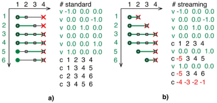
Fig. 2. Layout diagrams with cell indices on the vertical and vertex indices on the horizontal axis. A vertex is active from the time it is introduced until it is finalized, as indicated by the horizontal lines. (a) A standard format for tetrahedral meshes based on the OBJ format. (b) A streaming format that interleaves vertices with cells. Vertex finalization is provided with a negative index (i.e., relative to the most recent vertex).
Isenburg and Lindstrom [18] provide a streaming mesh format for triangle meshes that extends the popular OBJ file format. We use their format with additions to handle tetrahedral meshes. This includes extending the vertices to four values hx,y,z,fi that represent the position in 3D space and a scalar value. In addition, we provide a new element type for a tetrahedral cell that indexes four vertices. This format allows us to finalize a vertex when it is no longer in use by using a negative index into the vertex list. Figure 2 shows an ASCII example of the streaming tetrahedral format.
An important consideration with streaming meshes is the ability to analyze the efficiency of a mesh layout. Isenburg and Lindstrom developed several techniques for visualizing properties of the mesh to determine the effectiveness of the layout. We use similar tools to measure tetrahedral mesh quality. An important property is the front width, or the maximum number of concur-rently active vertices. An active vertex is one that has been introduced, but not yet finalized. The width of a streaming mesh gives a lower bound on the amount of memory required for dereferencing (and thus processing) the mesh. Another important property of the mesh is
the front span, which measures the maximum index
difference (plus one) of the concurrently active vertices. A low span allows a faster implementation because optimizations can be performed that achieve the best performance when the span is similar to the width. The efficiency of our layout depends on quantifying these properties, thus we provide analysis on different layout techniques so that we can choose the most streamable layout for a given data set.
One simple mesh layout is to sort the vertices on a
TABLE I
ANALYSIS OF MESH LAYOUT
Data Set Vertices Tetrahedra Spatial Sort Z-Order Spectral Breadth-First
Width Span Width Span Width Span Width Span
Torso 168,930 1,082,723 3,118 20,784 7,256 122,174 2,894 13,890 5,528 6,370
Fighter 256,614 1,403,504 3,894 110,881 9,382 215,697 3,916 28,638 16,629 19,523
Rbl 730,273 3,886,728 2,814 5,270 10,232 371,269 2,291 21,764 3,206 3,495
Mito 972,455 5,537,168 19,876 33,524 10,202 642,550 6,745 44,190 10,552 11,498
Sf1 2,461,694 13,980,162 16,898 65,921 48,532 1,958,212 12,851 131,152 30,258 33,378
tetrahedra. Wu and Kobbelt [16] use this technique for triangle mesh simplification. This can be accomplished for large meshes by performing an out-of-core sort on the vertices [15] and writing them into a new file. An additional file is created to contain a mapping of the old ordering to the new one. Next, the tetrahedral cells are written to a new file and re-indexed according to the mapping file. A sort is then performed on the file containing the tetrahedral cells based on the largest index of each cell. Finally, the vertex file and the cell file are read simultaneously and interleaved into a new file by writing each cell immediately after the vertex corresponding to the cell’s largest index has been written. Spatial layouts work especially well when considering meshes that have a dominant principal direction.
Other techniques may be desirable if the mesh does not have a dominant principal direction, such as a sphere. An approach to handle this type of data is to use a
bricking method similar to the one proposed by Cox and Ellsworth [20] in which the vertices are ordered into a fixed number of small cubes for better sequential access. A similar approach is to arrange the vertices using a Lebesgue space-filling curve (i.e., z-order), which pro-vides better sequential access in the average case. This arrangement can be generated by creating an out-of-core octree [21] of the vertices and traversing them in-order. The interleaved mesh is then written to a file in the same manner described above for spatial sorting. The results of the layout produced by bricking andz-order traversal are similar. When streamed they provide a more contiguous portion of the mesh on average, but the front width and span are typically much larger than sorting spatially.
Another approach used for laying out the mesh on disk is spectral sequencing. This heuristic finds the first non-trivial eigenvector (the Fiedler vector) of the mesh’s Laplacian matrix and was shown by Isenburg and Lindstrom [18] to be very effective at producing low-width layouts. They provide an out-of-core algo-rithm for generating this ordering for streaming triangle meshes, which we have extended to handle tetrahedra. This method works particularly well for curvy triangle
meshes, but tetrahedral meshes are generally less curvy and more compact. Still, in most cases this ordering results in the lowest width, which is ideal for minimizing memory consumption.
A final approach is to create a topological layout, which starts at a vertex on the boundary and grows out to neighboring vertices. To grow in a contiguous manner, we use a breadth-first traversal with optimizations to improve coherence. Instead of a traditional FIFO priority queue, we assign priority using three keys. First, the oldest vertex on the queue is used in the same way that it would be in standard breadth-first algorithms. However, if multiple vertices were added to the queue at the same time, a second and third key are used to achieve a more coherent order. The second key is boolean, and gives preference to a vertex if it is the final one in a cell that has not been processed. Finally, the third key is to use the vertex that was most recently put on the queue, which is more likely to be adjacent to the last vertex. These sort keys guarantee a layout that iscompact[18], such that runs of vertices are referenced by the next cell, and runs of cells reference the previous vertex (e.g.
as in Figure 2b). Using this approach, we were able to minimize the front span of the data sets in all of our experimental cases. This is ideal because having a span and width that are similar allows us to exploit optimization techniques described in the simplification algorithm.
Table I shows the front width and span for four differ-ent data sets produced by the layout techniques described above. Spectral sequencing proves to be the superior choice when low width and thus memory efficiency is required. Breadth-first layouts are not as memory-efficient, but as we will see can be processed fast. Note that unlike [17] we do not impose the constraint that the sequence of tetrahedra be grown in a face-adjacent manner (equivalently edge-face-adjacent for triangle meshes). Therefore we can accept a streaming mesh in whatever order it arrives without having to locally reorder elements.
III. TETRAHEDRALSIMPLIFICATION
A. Quadric-based Simplification
To achieve high-quality approximations, we use the quadric error metric proposed by Garland and Zhou [12]. This metric measures the squared (geometric and field) distances from points to hyperplanes spanned by tetrahe-dra. The volume boundaries are preserved using a similar metric on the boundary faces and by weighting boundary and interior errors appropriately. The generalized quadric error allows the flexibility of representing field data by extending the codimension of the manifold. Given a scalar function f :D⊆R3→Rdefined over a domainD
represented by a tetrahedral mesh, we can represent the vertices at each point p ashxp,yp,zp,fpi, which can be considered a point on a 3D manifold embedded in R4.
Thus, by extending the quadric to handle field data, the algorithm intrinsically optimizes the field approximation along with the geometric position.
The quadric error of collapsing an edge to a single point is expressed as the sum of squared distances to all accumulated incident hyperplanes, and can in n
dimensions be encoded efficiently as a symmetric n×n
matrixA, ann-vectorb, and a scalarc. It is sufficient to component-wise add these terms to combine the quadric error of two collapsed vertices. Finding the point x that minimizes this measure amounts to solving a linear system of equationsAx=b. Oncexis computed, we test whether collapsing to this point causes any tetrahedra to flip, i.e., changes the sign of their volume, in which case we disallow the edge collapse. Because A is not necessarily invertible, it is important to choose a linear solver that is numerically stable. Since quadric metrics are covered in great detail elsewhere (see, e.g. , [10], [12]), we here focus only on the numerical issues of robustly minimizing quadric errors (see Section III-D).
B. Streaming Simplification
Combining streaming meshes with quadric-based sim-plification, we introduce a technique for simplify-ing large tetrahedral meshes out-of-core. We base our streaming algorithm on [17], but make several general improvements and provide a list of optimizations that compared to a less carefully engineered implementation results in dramatic speed improvements.
First, unless already provided with streaming input, we convert standard indexed meshes and optionally reorder them for improved streamability. Then, portions of the streaming mesh are loaded incrementally into a fixed-size main memory buffer and are simplified using the quadric-based method. Once the in-core portion of the mesh reaches the user-prescribed resolution, simplified
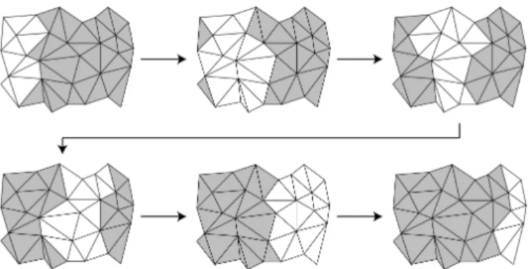
Fig. 3. Example of a buffer moving across the surface of a tetrahedral mesh sorted from left to right. As new tetrahedra are introduced, the tetrahedra that have been in-core the longest are removed from memory.
elements are output,e.g.to disk or to a downstream pro-cessing module. Thus input and output happen virtually simultaneously as the mesh streams through the memory buffer (see Figure 3).
To ensure that the final approximation is the desired size, two control parameters have been added: target reduction and boundary weight. Target reduction is the ratio between the number of tetrahedra in the output mesh and the number of tetrahedra in the original mesh. Alternatively, this parameter can be expressed as a target tetrahedral count of the resulting mesh. The boundary weight prevents the shape of the mesh from changing throughout the simplification. We use a fixed value of 100 times the maximum field value in the data for the weight in our experiments.
Because we only keep a small set of tetrahedra in memory, we do not know the entire mesh connectivity. Thus, we keep the boundary between the tetrahedra cur-rently in memory and all remaining elements—tetrahedra that have not yet been read or that have been output— fixed to ensure that the simplified mesh is crack-free. We call this boundary the stream boundary, which consists entirely of faces from the interior of the mesh. We can identify the stream boundary faces as they are read in by utilizing the finalization information stored in the streaming mesh. A face of the current in-core mesh is part of the stream boundary if none of its three vertices are finalized. We disallow collapsing any edge that has one or both vertices on the stream boundary.
Due to the stream boundary constraint, if we read in one portion of the mesh, simplify it, and write it out to disk in one phase, our output mesh will have unsimplified areas along the stream boundaries. This results in an approximation that is oversimplified in areas and under-simplified in others. To avoid this problem, we follow the algorithm proposed by Wu and Kobbelt [16]. Their
algorithm consists of a main loop in which READ, DEC-IMATE, and WRITE operations are performed in each iteration. The READ operation introduces new elements until it fills the buffer. Next, DECIMATE simplifies the elements in the buffer until either the target ratio is reached or the buffer size is halved. Finally, in their method the WRITE operation outputs the elements with the largest error to file.
We improve upon [16], [17] by ensuring, to the extent possible, that the relative order among input elements is preserved in the output stream, with the caveat that tetrahedra whose vertices have not yet been finalized (i.e., are on the input stream boundary) must be delayed. Therefore, the output typically retains the coherence of the input. An error-driven output criterion, on the other hand, can considerably fragment the buffer and split off small “islands” that remain in the buffer for a long time without being eligible for simplification, and thus unnecessarily clog the stream buffer. Furthermore, such an output stream generally has poor stream qualities, which affects downstream processing. The front width (i.e., number of active vertices), for example, is particu-larly important for tetrahedral meshes, for which each active vertex affects on average four times as many elements as in a triangle mesh, and therefore more adversely affects memory requirements and processing delay. Furthermore, we relax the requirement that the stream of tetrahedra (triangles) advance in a face (edge) adjacent manner [17], as this is of no particular value to us, and we allow any coherent ordering of mesh elements. Finally, using the more streamable layouts and simpler streaming mesh formats and API from [18], we gain considerably in performance and memory usage over [17].
C. Implementation Details
Since our method processes different mesh portions of bounded size sequentially, a statically allocated data structure is more efficient than dynamic allocations, which collectively increase the memory footprint. In our implementation, we extended Rossignac’s corner table [22] for triangle meshes to tetrahedral meshes. The original corner table requires two fixed-size arraysV and
O indexed by corners (vertex-cell associations)c, where
V[c] references the vertex of c and O[c] references the “opposite” corner of c.
In the case of tetrahedral simplification, the most common query is to find all tetrahedra around a vertex. Therefore, we replace the O array with a link table L
of equal size, which joins together all corners of a given vertex in a circular linked list. We additionally store with each vertex an index to one of its corners.
VERTEX
matrixA 10 floats
vectorp 4 floats
floatε
intidx global index
intcorner vertex-to-corner index
uchar f lags deleted, written
TETRAHEDRON
intvidx[4] vertex indices
intlink[4] corner links
booldeleted
intorder position in stream
Fig. 4. Data structures used for our quadric-based simplification.
We store the mesh internally as three fixed-size arrays of vertices, tetrahedra, and corners (i.e., the links L). Each vertex contains a pointer to one corner and the quadric error information (A,p,ε) using a
parameteri-zation that explicitly represents the vertex geometry and scalar data inp(see III-D and Figure 4). The quadrics for the tetrahedra are calculated when we read in a new set of tetrahedra, and are then distributed to the vertices. For each finalized vertex, we compute boundary quadrics for all incident boundary faces (if any) that have no other finalized vertices, and distribute these quadrics to the boundary vertices.
Garland and Zhou [12] use a greedy edge collapse method and maintain a priority queue for the edges or-dered by quadric error. Forsaking greediness, we obtain comparable mesh quality by using a multiple choice randomized approach [16] with eight candidates per col-lapse. There are several advantages of using randomized selection. One is that we no longer need a priority queue or explicit representation of edges. Instead an edge can be found by randomly picking a tetrahedron and then randomly selecting two of its vertices. Another advan-tage is that the randomized technique can be further accelerated by exploiting information readily available through our quadric representation (see III-D).
Before we output a tetrahedron, we must ensure that its four vertices are output first. Once a vertex is output, we mark it for not being decimated in future iterations. To enhance the performance, we use a lazy deletion scheme, where all vertices and tetrahedra to be deleted are initially marked. At the end of each WRITE phase, we make a linear pass through all vertices and tetrahedra to remove marked elements and compact the arrays. Since we do not allocate additional memory during simplification, keeping deleted vertices and tetrahedra does not increase the memory footprint.
TABLE II
IMPLEMENTATIONIMPROVEMENTS
Improvements Time Memory (sec) (MB) Initial Implementation 212.95 310
QEF + CG 132.68 282
Multiple Choice + Corner Table 38.35 130
4D Normal, Floats 35.99 78
Final / Binary I/O 22.10 78
Storing large data sets on disk in ASCII format can adversely affect performance because converting ASCII numbers to an internal binary representation can be surprisingly slow. We have extended the ASCII stream format in Figure 2 to a binary representation. Because our program spends over 30% of the time on disk I/O, this optimization results in a non-negligible speedup. For example, on the SF1 data set it improves overall performance by 17%.
Since we only maintain a small portion of the mesh in-core, we require a way of mapping global vertex indices to in-core buffer indices. Usually a hash map is used, but with our low-span breadth-first mesh layout, this hash map can be replaced by a fixed-size array indexed using modular arithmetic. We move occasional high-span vertices that cause “collisions” in this circular array to an auxiliary hash.
With all of the optimizations described above, our simplifier can run at high speed without any dynamic memory allocation at run time. The performance and memory summary can be found in Table II. The results are for simplifying the Fighter data set (1.4 M tetrahedra) completely in-core on a P4 2.2GHz with 1GB of RAM. Further efficiency improvements relating to quadric error metrics will be discussed in the following section.
D. Numerical Issues
Great care has to be taken when working with quadric metrics to ensure numerical stability while retaining effi-ciency. To minimize quadric errors, a positive semidefi-nite system of linear equations must be solved, for which numerically accurate but heavy-duty techniques such as singular value decomposition (SVD) [13], [23] and QR factorization [24] have been proposed. However, even constructing, representing, and evaluating quadric errors require that special care be taken. We here outline an efficient representation of quadric error functions that leads to numerically stable operations, improved speed, and less storage.
The standard representation [12] of quadric errors is
SOLVE(A,x,b,n,κmax)
1 r=b−Ax negative gradient ofQ
2 p=0
3 fork=1, . . . ,n iterate up tontimes
4 s=rTr
5 ifs=0 then exit solution found?
6 p=p+r/s update search direction
7 q=Ap
8 t=pTq
9 ifst≤tr(A)/(nκmax)then exit insignificant direction?
10 r=r−q/t update gradient
11 x=x+p/t update solution
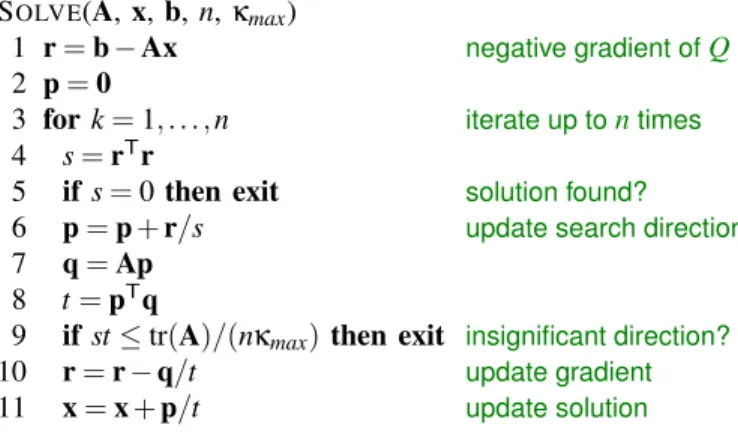
Fig. 5. Conjugate gradient solver for positive semidefinite systems Ax=b. On inputxis an estimate of the solution,n=4 is the number of linear equations, andκmax is a tolerance on the condition number.
tr(A)is the trace ofA.
parameterized by (A,b,c), and is evaluated as
Q(x) =xTAx−2bTx+c (1) Typically the three terms in this equation are “large,” but sum to a “small” value, resulting in a loss of precision. One can show that the roundoff error is proportional to kAkkxk2. Furthermore, in addition to this quadric information, it is common to store the vertex position (and field value) p that minimizes Q separately. Lind-strom [25] suggested an alternative representation that removes this redundancy:
Q(x) = (x−p)TA(x−p) +ε (2)
where A is the same as in the standard representation and
Ap = b
pTAp+ε = c
This parameterization (A,p,ε) provides direct access
to the minimum quadric error ε and the minimizer
p. This not only saves memory but also results in a more stable evaluation of Q, as the roundoff error is now proportional to kAkkx−pk2, and we are generally interested in evaluating Q(x) near its minimum p as opposed to near the origin. Another significant benefit of this representation is that it provides a lower bound
εi+εj onQi+Qj when collapsing two verticesviandvj.
Using randomized edge collapse [16], we can thus often avoid minimizing Qi+Qj if the lower bound already
exceeds the smallest quadric error found so far.
Our quadric representation also lends itself to an efficient and numerically stable iterative linear solver. To handle ill-conditioned matrices A, we have adapted the well-known conjugate gradient (CG) method [26] to work on semidefinite matrices. As in SVD, we provide
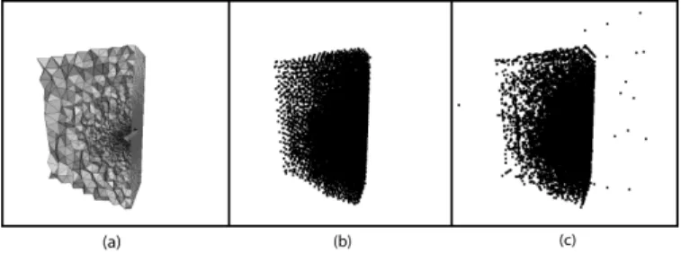
Fig. 6. Demonstration of the stability of linear system solvers on the Fighter data set. A portion of the original mesh is shown in (a). Solutions to linear equations are shown as black dots using SVD with Cramer’s Rule (b) and Cholesky factorization (c).
TABLE III
PERFORMANCE OF LINEAR SOLVERS
Linear System Solver Performance Stability
Cholesky 0.94 sec Unstable
SVD 2.86 sec Stable
SVD with Cramer’s Rule 1.16 sec Stable Conjugate Gradient 1.0 sec Stable
a tolerance κmax on the condition number κ(A), and
preempt the iterative solver when all remaining conjugate directions are deemed “insignificant” for reducing Q. This is equivalent to zeroing small singular values in SVD. Using our quadric representation, we conveniently initialize the CG solver with the guess x= (pi+pj)/2.
A final word of caution: The computation of gener-alized quadrics presented in [12] computes A = I - N, whose null space null(A) =range(N) is spanned by the tetrahedron, via subtraction, which due to roundoff error can leave A indefinite, i.e., with one or more negative eigenvalues. This causes Q to have a “saddle” shape with no defined minimum, and can cause numerical instability. Instead, we compute a 4D “volume normal” using a generalization of the 3D cross product to 4D. The outer product of this normal with itself gives a positive semidefinite Afor a tetrahedron.
Because of our attention to numerical stability, with
κmax =103 we are able to use single precision floating
point throughout our simplifier, even for the largest meshes. Since the 4D quadric information requires 15 scalars per vertex, this saves considerable memory and improves the speed.
IV. RESULTS
A. Stability and Error Analysis
We have described a CG method for solving the linear equations that arise when minimizing the quadric error. The choice of solver is important because degenerate tetrahedra and regions of near-constant field value can cause singularity. For testing purposes, we constructed
Fig. 7. Volume Rendered images of the Fighter data set show the preservation of scalar values. The original data set is shown on the left (1,403,504 tetrahedra) and the simplified version is shown on the right (140,348 tetrahedra).
a data set by subdividing a tetrahedron into hundreds of smaller tetrahedra by interpolating the vertices and field data. Obviously, these small tetrahedra all lie on the hyperplane spanned by the original tetrahedron, thus they are solutions to the linear equations. We then picked a solution as a target for each collapsed edge. We exper-imented with several linear solvers as shown in Table III and Figure 6. The results are for simplifying the Fighter data set (1.4 M tetrahedra) completely in-core. We experimented with Cholesky factorization, SVD, SVD with Cramer’s Rule, and CG. Our hybrid SVD/Cramer’s Rule method uses a conservative condition estimator and uses Cramer’s Rule when the matrix is well-conditioned. Using all of our solvers, we were able to simplify our subdivided tetrahedron to its original shape with small error in both field and geometry. In our experiments, CG provides the fastest, most stable solution.
To estimate the error in the simplified mesh we use two different methods. The first method is to measure the error on the surface boundary of the mesh using the tool Metro [27]. The second method is to measure the error in the field data using a similar approach to Cignoniet al. [9]. Our implementation differs because it ignores points outside the domain of the simplified mesh since these points become part of the surface boundary error. Table IV shows these measured error estimations. Field error percentages are in relation to the range of the field and surface error percentages are in relation to the bounding box diagonal. Figure 7 shows an example of the quality of the resulting field and Figure 8 shows an example of the quality of the resulting surface.
B. Performance
All timing results were generated on a 3.2 GHz Pentium 4 machine with 2.0 GB RAM. For the streaming experiments, we limit the operating system to only 64 MB RAM by using the Linux bootloader. Table IV
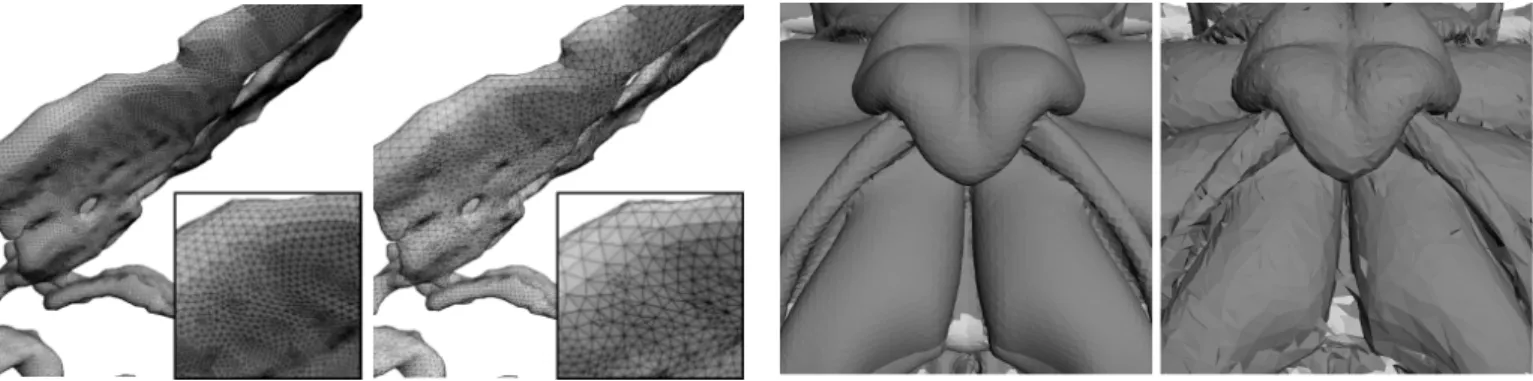
Fig. 8. Views of the mesh quality on the surface of the Rbl data set. The original data set is shown on the left (3,886,728 tetrahedra) and the simplified version is shown on the right (388,637 tetrahedra).
shows the results of simplifying a collection of data sets to 10% of their original size using our streaming algorithm and the same implementation optimized for in-core execution.
We were able to achieve streaming simplification with only a slight increase in time and error compared to an in-core implementation. The streaming technique has the advantage of a smaller memory footprint. With our algorithm, we were able to simplify 14 million tetrahedra while only using 20 MB RAM. Due to the large size of the Sf1 data set, certain parts of the stream were not able to be simplified accurately, resulting in a larger error. By increasing the memory slightly, the quality of the simplification is greatly improved and approaches the in-core quality.
C. Large-Scale Experiment
Although extremely large meshes exist, it is difficult to obtain unclassified access to them. To stress our algorithm on current PC hardware and to demonstrate the scalability of the technique, we performed streaming simplification on a huge fluid dynamics data set. The data set was created from sampling slices of a 20483 simulation and consists of over one billion tetrahedra that use 18 GB of disk space when stored in the binary format. The tetrahedra were laid out in the order in which they were sliced, which is comparable to sorting by axis. An in-core approach to simplifying this data set would require a machine with 64 GB RAM. We were able to simplify the data using only 829 MB RAM to 12 million tetrahedra (1.2%) in 10 hours on our test machine. Because error estimations were not possible with the entire data set in-core, we computed the field error on subregions of the mesh separately to verify the results. In the regions that were measured, there was 10.85% maximum and 1.57% RMS field error. Figure 9 shows an isosurface extracted from the original and
Fig. 9. Isosurfaces of the fluid dynamics data set. A portion of the original data set is shown on the left (over a billion tetrahedra) and a portion of the simplified data set is shown on the right (12 million tetrahedra). The numerical error in the simplified version is negligible (1.57% RMS).
simplified fluid dynamics data set. V. DISCUSSION
The use of streaming meshes for simplification re-duces the memory footprint of a large mesh considerably. We improved on the algorithm of Wu and Kobbelt [16] by preserving the stream order of the mesh between input and output. A direct comparison with their algorithm shows that our method consistently achieves a lower width, e.g. 9% versus 59% on the Fighter data set, and span,e.g.45% versus 98%, without reducing the approx-imation quality. In addition, with the optimizations that we employ to our data structures, we have been able to simplify up to 14 million tetrahedra while using only 20 MB RAM. Only the smallest data sets (Torso and Fighter) could be simplified using our implementation of Wu and Kobbelt’s algorithm.
Apart from providing a streaming algorithm that oper-ates on meshes of arbitrary size, we also described speed and stability optimizations that improve the performance of tetrahedral simplification. Our quadric representation improves linear solver performance. In addition, our adapted conjugate gradient method and the use of “vol-ume normals” for tetrahedra reduce the n“vol-umerical errors and allow the use of single precision floating-point num-bers. By using a binary format, we improve on storage and speed up I/O. Finally, through the use of a breadth-first mesh layout, we have improved the width and the span, which enables the use of a fixed-size circular array instead of a hash table. With these improvements, we have improved the speed of our simplification method by an order of magnitude over our initial implementation of Garland and Zhou’s quadric-based simplification [12].
Due to the efficiency of our algorithm, we easily handle the largest data sets we obtained. In our experi-mental results, our streaming algorithm simplifies about
TABLE IV
IN-CORE AND STREAMING SIMPLIFICATION RESULTS
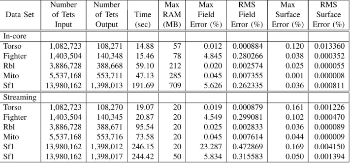
Number Number Max Max RMS Max RMS
Data Set of Tets of Tets Time RAM Field Field Surface Surface
Input Output (sec) (MB) Error (%) Error (%) Error (%) Error (%) In-core Torso 1,082,723 108,271 14.88 57 0.012 0.000884 0.120 0.013360 Fighter 1,403,504 140,348 15.46 78 4.845 0.280266 0.038 0.000352 Rbl 3,886,728 388,668 59.10 212 0.020 0.002574 0.025 0.000055 Mito 5,537,168 553,711 47.13 285 0.045 0.007355 0.001 0.000008 Sf1 13,980,162 1,398,013 191.69 709 5.626 0.262335 0.036 0.000811 Streaming Torso 1,082,723 108,270 19.07 20 0.019 0.000879 0.161 0.001226 Fighter 1,403,504 140,345 20.87 20 4.549 0.299081 0.102 0.000470 Rbl 3,886,728 388,671 95.54 20 0.025 0.002833 0.036 0.000089 Mito 5,537,168 553,716 73.58 20 0.045 0.007614 0.044 0.000009 Sf1 13,980,162 1,398,012 246.15 20 23.287 0.472869 0.169 0.004150 Sf1 13,980,162 1,398,017 244.42 50 5.834 0.315583 0.050 0.001394
60K tetrahedra per second and achieves high quality results. Given a machine with 2.0 GB of RAM, the in-core implementation of our algorithm could handle ap-proximately 35 million tetrahedra. Using our streaming method, we were able to simplify a data set consisting of almost one billion tetrahedra to one percent using only about 800 MB of RAM with very small error. The maximum bound of the streaming algorithm is only constrained by the front width of the mesh, which we have shown to be very small when using a good mesh layout.
VI. CONCLUSIONS ANDFUTUREWORK We have presented a streaming technique for simpli-fying tetrahedral meshes of arbitrary size. We describe several methods for laying out a tetrahedral mesh on disk in a coherent, I/O-efficient format. We also show an analysis of these layouts and the effects they have on the final simplified mesh. We provide a technique for simplifying small portions of the mesh in memory while obtaining a smooth simplification over the entire mesh. The simplification occurs in one pass, preserves mesh topology and scalar information, requires little memory, and runs quickly. We also provide optimizations to traditional simplification data structures that improve speed and efficiency. We present a linear solver that improves stability and speed of quadric-based simplifi-cation. Finally, we provide stability and error analysis of our algorithm with results for specific examples that show the time and memory required for processing.
Because the generalized quadric error works on a variety of data types, an interesting extension would be to attempt to handle meshes consisting of other types,
e.g. hexahedra. Finally, it would be interesting to take advantage of the coherent streaming tetrahedral format to perform fast, out-of-core isosurface extraction.
VII. ACKNOWLEDGMENTS
This work was performed under the auspices of the U.S. DOE by LLNL under contract no. W-7405-Eng-48. We would like to thank Jason Shepherd for the Rbl and Mito data sets and Louis Bavoil for the error analysis code. We also thank NASA for the Langley Fighter data set and Rob MacLeod at University of Utah for the Torso data set. Huy T. Vo is funded by the National Science Foundation Research Experiences for Undergraduates (REU) program. Steven P. Callahan is supported by the Department of Energy (DOE) under the ASC VIEWS program. Cláudio T. Silva is partially supported by the DOE under the ASC VIEWS program, the National Sci-ence Foundation (grants CCF-0401498, EIA-0323604, OISE-0405402, IIS-0513692, CCF-0528201), an IBM Faculty Award, and a University of Utah Seed Grant.
REFERENCES
[1] I. J. Trotts, B. Hamann, K. I. Joy, and D. F. Wiley, “Simplifi-cation of tetrahedral meshes,” inIEEE Visualization ’98 (VIS ’98). Washington - Brussels - Tokyo: IEEE, Oct. 1998, pp. 287–295.
[2] I. J. Trotts, B. Hamann, and K. I. Joy, “Simplification of tetrahedral meshes with error bounds,” in IEEE Transactions on Visualization and Computer Graphics. IEEE Computer Society, 1999, vol. 5 (3), pp. 224–237.
[3] A. V. Gelder, V. Verna, and J. Wilhelms, “Volume decimation of irregular tetrahedral grids,”Computer Graphics International, pp. 222–230, 1999.
[4] D. Uesu, L. Bavoil, S. Fleishman, and C. T. Silva, “Simplifi-cation of unstructured tetrahedral meshes by point-sampling,” Scientific Computing and Imaging Institute, University of Utah, Tech. Rep., 2004, uUSCI-2004-005.
[5] H. Hoppe, “Progressive meshes,” inProceedings of SIGGRAPH 96, ser. Computer Graphics Proceedings, Annual Conference Series, Aug. 1996, pp. 99–108.
[6] J. Popovi´c; and H. Hoppe, “Progressive simplicial complexes,” in Proceedings of the 24th annual conference on Computer graphics and interactive techniques. ACM Press/Addison-Wesley Publishing Co., 1997, pp. 217–224.
[7] O. G. Staadt and M. H. Gross, “Progressive tetrahedralizations,” inIEEE Visualization ’98, 1998, pp. 397–402.
[8] P. Chopra and J. Meyer, “Tetfusion: an algorithm for rapid tetrahedral mesh simplification,” in IEEE Visualization ’02. IEEE Computer Society, 2002, pp. 133–140.
[9] P. Cignoni, D. Constanza, C. Montani, C. Rocchini, and R. Scopigno, “Simplification of tetrahedral meshes with ac-curate error evaluation,” in IEEE Visualization ’00. IEEE Computer Society Press, 2000, pp. 85–92.
[10] M. Garland and P. S. Heckbert, “Surface simplification using quadric error metrics,” in Proceedings of SIGGRAPH 97, ser. Computer Graphics Proceedings, Annual Conference Series, Aug. 1997, pp. 209–216.
[11] V. Natarajan and H. Edelsbrunner, “Simplification of three-dimensional density maps,”IEEE Transactions on Visualization and Computer Graphics, 2004, to appear.
[12] M. Garland and Y. Zhou, “Quadric-based simplification in any dimension,”ACM Transactions on Graphics, vol. 24, no. 2, Apr. 2005.
[13] P. Lindstrom, “Out-of-core simplification of large polygo-nal models,” in Proceedings of the 27th annual conference on Computer graphics and interactive techniques. ACM Press/Addison-Wesley Publishing Co., 2000, pp. 259–262. [14] J. Rossignac and P. Borrel, Geometric Modeling in Computer
Graphics. Springer-Verlag, 1993, ch. Multi-resolution 3D approximations for rendering complex scenes, pp. 455–465. [15] P. Lindstrom and C. T. Silva, “A memory insensitive technique
for large model simplification,” inProceedings of the conference on Visualization ’01. IEEE Computer Society, 2001, pp. 121– 126.
[16] J. Wu and L. Kobbelt, “A stream algorithm for the decimation of massive meshes,” in Graphics Interface ’03 Conference Proceedings, 2003, pp. 185–192.
[17] M. Isenburg, P. Lindstrom, S. Gumhold, and J. Snoeyink, “Large mesh simplification using processing sequences,” in Visualization’03 Conference Proceedings, 2003, pp. 465–472. [18] M. Isenburg and P. Lindstrom, “Streaming meshes,” Lawrence
Livermore National Laboratory, Tech. Rep., 2005, uCRL-CONF-211608 to appear in Visualization’05.
[19] A. Mascarenhas, M. Isenburg, V. Pascucci, and J. Snoeyink, “Encoding volumetric grids for streaming isosurface extrac-tion,” in International Symposium on 3D Data Processing, Visualization, and Transmission ’04 Proceedings, 2004. [20] M. Cox and D. Ellsworth, “Application-controlled
demand paging for out-of-core visualization,” in IEEE Visualization ’97, 1997, pp. 235–244. [Online]. Available: citeseer.ist.psu.edu/cox97applicationcontrolled.html
[21] P. Cignoni, C. Montani, C. Rocchini, and R. Scopigno, “Exter-nal memory management and simplification of huge meshes,” IEEE Transactions on Visualization and Computer Graphics, vol. 9, no. 4, pp. 525–537, 2003.
[22] J. Rossignac, “3d compression made simple: Edgebreaker with zip&wrap on a corner-table,” in 2001 Proceedings of the International Conference on Shape Modeling & Applications. Washington, DC, USA: IEEE Computer Society, 2001, p. 278. [23] L. P. Kobbelt, M. Botsch, U. Schwanecke, and H.-P. Seidel, “Feature-sensitive surface extraction from volume data,” in Proceedings of ACM SIGGRAPH 2001, ser. Computer Graphics Proceedings, Annual Conference Series, Aug. 2001, pp. 57–66. [24] T. Ju, F. Losasso, S. Schaefer, and J. Warren, “Dual contouring of hermite data,”ACM Transactions on Graphics, vol. 21, no. 3, pp. 339–346, July 2002.
[25] P. Lindstrom, “Out-of-core construction and visualization of multiresolution surfaces,” in2003 ACM Symposium on Inter-active 3D Graphics, Apr. 2003, pp. 93–102.
[26] G. H. Golub and C. F. Van Loan,Matrix Computations, 3rd ed. Johns Hopkins University Press, 1996.
[27] P. Cignoni, C. Rocchini, and R. Scopigno, “Metro: measuring error on simplified surfaces,” Computer Graphics Forum, vol. 17, no. 2, pp. 167–174, 1998. [Online]. Available: http://vcg.sourceforge.net/tiki-index.php?page=Metro