The Issuance of sTaTe and LocaL debT durIng The
unITed sTaTes greaT recessIon
Ronald C. Fisher and Robert W. Wassmer
This research explores the borrowing behavior of state and local governments between 2008 and 2010, a period that encompasses the Great Recession. State and local governments continued to borrow markedly during this period of severe fiscal stress. Following an overview of state-local debt and subnational government bor-rowing, we present a statistical analysis of the demographic, economic, political, and institutional factors that influenced interstate differences in borrowing. This research suggests that both economic and political factors influenced borrowing and that the availability of Build America Bonds contributed to an increase in bor-rowing during this period.
Keywords: state-local borrowing, state-local debt, Build America Bonds JEL Codes: H11, H74, H77
I. IntroductIon
T
he objective of this research is to explore the borrowing behavior of state and local governments between 2008 and 2010, a period that encompasses the Great Reces-sion that officially occurred between December 2007 and June 2009.1 Three issues are of particular interest. First, this was an extraordinary period, creating fiscal problems for state and local governments unprecedented in at least the previous 30 years. A number of authors have explored how states and localities responded fiscally to the Great Recession, but the focus of this paper, which we believe to be unique, is that itRonald C. Fisher: Department of Economics, Michigan State University, East Lansing, MI, USA and Zhongnan University of Economics and Law, Wuhan, CHINA ([email protected])
Robert W. Wassmer: Department of Public Policy and Administration, California State University, Sacra-mento, CA, USA ([email protected])
1 The explicit focus of this paper is on financial market debt through the issuance of interest-bearing bonds and notes. This paper does not consider other forms of debt, including the future pension costs and post-retirement health care costs of past and current employees or internal borrowing, transferring money from some internal dedicated funds with surpluses to a general fund or other uses.
explicitly examines borrowing behavior during this period. Although subnational gov-ernments in the United States avoided potentially large deficits through a combination of substantial spending reductions and modest (in most states) tax increases during this recession, these governments continued to issue bonds to finance new debt and refinance existing debt, which may seem counterintuitive. Such borrowing might be expected if states borrowed to avoid deficits and/or fund stimulus policy. Alternatively, subnational governments might have restrained borrowing if there was concern about long-term balanced budgets and persistent revenue shortfalls or if the overall economic slowdown created a lower demand for public capital.
A second reason to pay special attention to this period is the dramatic changes that occurred in several aspects of municipal bond finance. Perhaps of greatest interest is the fact that state and local governments possessed the ability for a limited period to issue Build America Bonds (BABs). Available only between April 2009 and December 2010, BABs were bonds in which interest paid to borrowers counted as taxable income, but whose issuers received a direct federal government subsidy of 35 percent of their interest payments.2 Although there have been proposals for the use of subsidized tax-able state-local bonds (Galper and Peterson, 1973), this was the first broad application available to all state and local governments in the United States.
Third, market conditions were unique during this period. Interest rates in general, and those applying in particular to state and local bonds, reached historic lows during the Great Recession due to the policies of the Federal Reserve. Not only did the level of interest rates decline, but the rates paid by municipal borrowers relative to those paid by the Treasury and corporate borrowers also fluctuated substantially. Furthermore, as Ely (2012) notes, the use of bond insurance by state and local governments fell sub-stantially during and after the financial market crisis, which some might expect to affect borrowing behavior. Changes in the insurance market for bonds were a result of the severity of the recession, the general decline in interest costs, changes in credit rating practices, and even the opportunity offered by BABs. Clearly this was an unusual time for financial markets. Although all of these factors make this an especially interesting time to study state and local debt, they also complicate the analysis.
The research that follows provides more recent evidence for the differences among states in annual borrowing by subnational governments. A statistical analysis presents evidence about the demographic, economic, political, and institutional factors that influ-enced interstate differences in borrowing during the Great Recession, supplementing existing empirical findings about why some states use more subnational debt than others. The remainder of the paper is divided into seven sections. The next section offers a broad description of state and local debt in the United States from 1992 to 2007. Section III describes subnational government borrowing at the time of the Great Recession. In Section IV, we formulate and estimate a regression model drawing on the relevant literature on what determines differences in state and local bond issues, state institutional 2 For details regarding the Build America Bonds program, see Mercator Advisors (2009) and Luby (2012).
and financial procedures that influence bond borrowing costs, and the limited research already conducted on Build America Bonds. Section V presents the regression results, while Section VI concludes with a brief summary and some policy implications.
II. State and LocaL Government debt before the Great receSSIon
To put subnational government borrowing in the United States between 2008 and 2010 in context, it is useful to review the previous status of such debt.3 In 2007, state and local governments had accumulated financial market debt of nearly $2.5 trillion, or about $8,300 per person. This subnational debt amounted to about 17 percent of U.S. Gross Domestic Product (GDP), and nearly 79 percent of the annual revenue collected by all state and local governments in the country. From 1992 to 2007, state and local government debt increased relative to both population and GDP, but did not increase relative to the total revenue of state and local governments. In 2007, before the effects of the recession, aggregate state and local government debt amounted to about 79 percent of state and local revenue, roughly the same level as in 1992 and 1997. Comparing fiscal years 1997 and 2007 seems appropriate as both came after a period of rapid economic growth. Thus, as of 2007, state and local governments in aggregate had not incurred outstanding debt historically disproportionate to their annual budgets.
Annual interest payments on the outstanding debt of subnational governments in the United States decreased as a share of revenue from 1992 to 2007 for all types of state and local governmental units except for school districts, where interest payments as a share of revenue remained roughly constant. Most of the increase in state and local debt between 1992 and 2007 was long-term debt for public purposes, especially debt incurred by K–12 school districts. School district long-term debt increased from 6 percent of total state and local long-term debt in 1992 to 13 percent in 2007.
III. overvIew of SubnatIonaL borrowInG durInG the Great receSSIon
Figure 1 lists state and local government bond issues by year for 2005 through 2011. In this figure state and local issues are combined but separated into the categories of short-term bonds (with a maturity date of less than one year), long-term bonds (exclud-ing Build America Bonds), and BABs. Aggregate state and local government debt is examined, rather than the debt incurred by state governments alone, as the latter offers misleading comparisons across the states. States differ dramatically in the degree to which the state or its local governments take responsibility for generating revenue, providing public services, and issuing debt. Some state government authorities incur debt on behalf of their local governments whereas in other states, local governments are responsible for incurring debt directly. In some states, local governments can only incur 3 Prior research on state-local debt is described in Wassmer and Fisher (2011a, b).
debt after approval of the state government. In every state, state governments distribute state revenue to local governments in the form of intergovernmental grants that differ widely in magnitude. These factors suggest legal, economic, and political links between the fiscal behavior of a state government and its local governments that differ in every state; accordingly, when making interstate comparisons of debt issuance we consider the combined state and local government sector as a single entity.4
Focusing only on long-term debt (including Build America Bonds), new issues declined substantially in 2008 (the first year of the Great Recession and a period with substantial uncertainty in the financial markets). Subsequently, the volume of long-term bonds (including BABs) issued by state and local governments rose in both 2009 and 2010. In terms of the total bond volume, 2010 was similar to 2007 (the year prior to the financial market crisis and start of the Great Recession). The substantial magnitude of
448.4 411.7 444.8 388.2 345.5 261.6 308.8 64.2 178.6 55.5 46.9 60.0 60.6 64.7 65.3 63.5 0 100 200 300 400 500 600 2005 2006 2007 2008 2009 2010 2011 2009$ Billions Calendar Year
Long-term Issues, Excluding BABs Build America Bonds Short-term Issues
Source: “Market Statistics,” The Bond Buyer, New York, NY, http://www.bondbuyer.com/marketstatistics/
#SemiannualandAnnualStatistics
figure 1
Real State-Local Bond Issues, by Type and Year
4 Unfortunately, there are limited details available regarding state institutional differences in borrowing practices. We do our best to control for these details in the empirical analysis.
Build America Bonds during this period is clear. In 2010, BABs accounted for nearly a quarter of all state and local borrowing. Figure 1 also illustrates that real long-term borrowing by state and local governments decreased dramatically in 2011. One pos-sible explanation is the moving up of planned 2011 capital projects, and the associated borrowing to finance them, to 2010 due to the availability of Build America Bonds. A second possibility is that state and local governments were being exceptionally cautious in the aftermath of the recession and the uncertain fiscal situation that still existed.5
The pattern for municipal bond issuance around the recession of 2001 was a bit dif-ferent. Bond issuance did not decline during the initial year of the recession, neither in fiscal year 2001 or fiscal year 2002 using Census data nor calendar year 2001 using data from the Securities and Financial Markets Association. Indeed, bond issuance increased substantially during calendar years 2001 and 2002 and during fiscal and years 2002 and 2003 (the recession was from March 2001 through November 2002). Bond issuance continued to increase in fiscal and calendar year 2003 before stabilizing in 2004. The large decline seen in 2011 did not occur following the 2001 recession.
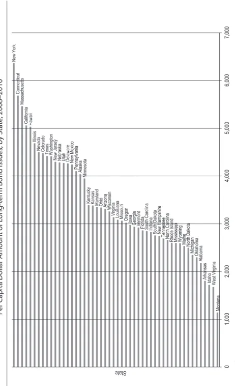
As shown convincingly in Figure 2, interstate differences in per capita borrowing over the three-year period of 2008 through 2010 were substantial, varying from about $7,400 per capita in New York to less than $1,200 per capita in Montana. Such variance indicates that population alone is not enough to standardize a comparison of borrowing among the states. Furthermore, although some states with relatively high per capita debt in 2007 (such as New York and Massachusetts) were relatively heavy borrowers in the three years that followed, others with relatively high per capita debt (such as Rhode Island) were not.
Table 1 provides a comparison for all states of each specific state’s share of the national total of subnational long-term bond issues during 2008 through 2010 and each state’s share of national total outstanding debt (the result of past long-term bond issues) in 2007. Table 2 provides a similar perspective, but only for BABs. The last column in Table 1 displays the ratio of the 2008 to 2010 percentages of a state’s new subnational bond issues relative to all states divided by the percentage of the same state’s outstanding debt in 2007 relative to all states. In this last column, a ratio greater than one indicates that subnational governments in that state made relatively more use of borrowing during the 2008 to 2010 period than they had in a previous long-run period. For the 20 or so states at both ends of the distribution, the differences are substantial. For instance, the relative borrowing of New Mexico, Nebraska, Utah, Hawaii, and Iowa from 2008 to 2010 (relative to the aggregate borrowing of all states) was at least 25 percent greater than past borrowing as reflected by relative outstanding debt in 2007. There are several possible explanations for the pattern of interstate variation observed in Figure 2 and Table 1. One possibility is that because borrowing for capital expenditures in a state 5 A sample comment reflecting this view is “… a newfound sense of fiscal austerity gripped state and local governments and that discouraged any willingness to take on additional debt …” (“2011 in Statistics,” The Bond Buyer, New York, NY, http://www.bondbuyer.com/specialreports).
figur e 2 Per C apita D ollar A moun t of L ong-t er m B ond Issues , b y S ta te , 2008–2010* Not e: These figur
es include both non-taxable and Build A
mer ica B ond issues . Sour ce: P ro vided pr iv at ely b y Thomson R eut ers , h ttp://thomsonr eut ers .c om/pr oduc ts_ser vic es/financial Montana West Virginia Idaho Arkansas New York Connecticu t Massachusetts California Hawaii Illinois
Nevada Colorado Texas Washington New Jersey Nebraska Utah Delawar
e New Mexic o Pennsylvania Alaska Ohio Maryland Kansas Kentucky Minnesot a Arizon a Wisconsin
Virginia Louisiana Missour
i
Oregon Iowa
Georgia Vermont Florida South Carolina Indiana South Dakota New Hampshir
e
Tennesse
e
North Carolina Rhode Island Mississippi Wyoming Maine North Dakota
Michigan Oklahoma Alabama 01 ,000 2,000 3,000 4,000 5,000 6,000 7,000 State
table 1
Long-Term Bond Issue in 2008 to 2010 Relative to Historic Use of Debt
State (1) Percentage of U.S. Long-term State-local Borrowing 2008–2010 (2) Percentage of U.S. Outstanding State-local Debt 2007 Ratio of (1) to (2) New Mexico 0.79 0.51 1.56 Nebraska 0.67 0.48 1.41 Utah 0.91 0.66 1.38 Hawaii 0.55 0.43 1.28 Iowa 0.78 0.61 1.27 Connecticut 1.68 1.36 1.24 Mississippi 0.65 0.52 1.24 Wyoming 0.11 0.09 1.21 Georgia 2.40 2.01 1.19 Texas 9.25 7.86 1.18 California 15.65 13.70 1.14 Arizona 1.86 1.63 1.14 Minnesota 1.79 1.61 1.11 Maryland 1.59 1.43 1.11 Louisiana 1.26 1.17 1.08 North Carolina 2.15 2.08 1.03 Oklahoma 0.71 0.69 1.03 Nevada 0.94 0.92 1.03 Ohio 2.90 2.83 1.03 Idaho 0.22 0.22 1.00 Tennessee 1.41 1.41 1.00 Illinois 4.80 4.84 0.99 Pennsylvania 4.55 4.64 0.98 New York 10.48 10.77 0.97 Kansas 0.79 0.82 0.97 Virginia 2.03 2.12 0.96 Colorado 1.84 1.92 0.96 Vermont 0.16 0.17 0.95 Missouri 1.48 1.61 0.92 Washington 2.36 2.58 0.91 North Dakota 0.14 0.15 0.91 Wisconsin 1.55 1.74 0.89 New Jersey 3.15 3.56 0.89 South Dakota 0.18 0.20 0.88 Maine 0.29 0.33 0.88 Arkansas 0.44 0.51 0.86 Indiana 1.49 1.72 0.86 Delaware 0.32 0.37 0.86
or a local government may not happen uniformly over time (i.e., it is “lumpy”), the 2008 to 2010 period is not representative of the long-run situation for any given state. In that case, the data simply represent those states that were borrowing heavily during this period. However, because these borrowing data cover a three-year period and are aggregated for all subnational governments in each state, the level of aggregation may sufficiently offset the “lumpy” nature of borrowing and suggest correctly whether state behavior in this period was different than in the past.6
In Table 2, a few large users of BABs stand out. Subnational governments in Califor-nia issued almost 21 percent of all Build America Bond volume, which was more than 50 percent greater than California’s share of outstanding debt in 2007. Similarly, the large population states of New York, Illinois, Ohio, and Washington (all states with a relatively substantial historic shares of aggregate debt) made even greater relative use of the federally subsidized BABs opportunity. One possible explanation for why large
table 1 (continued)
Long-Term Bond Issue in 2008 to 2010 Relative to Historic Use of Debt
State (1) Percentage of U.S. Long-term State-local Borrowing 2008–2010 (2) Percentage of U.S. Outstanding State-local Debt 2007 Ratio of (1) to (2) Alabama 0.86 1.02 0.85 Oregon 1.00 1.20 0.84 Massachusetts 3.02 3.72 0.81 Kentucky 1.23 1.53 0.80 Florida 4.44 5.56 0.80 South Carolina 1.08 1.49 0.72 New Hampshire 0.30 0.43 0.71 West Virginia 0.26 0.38 0.70 Michigan 1.99 3.03 0.65 Rhode Island 0.25 0.44 0.59 Alaska 0.24 0.41 0.58 Montana 0.09 0.26 0.37
Sources: Provided privately by Thomson Reuters, http://thomsonreuters.com/products_services/ financial, and the U.S. Census Bureau, State and Local Government Finances, 2007, http://www. census.gov/govs/local
6 In fact, we know from other work (Wassmer and Fisher, 2011a, 2011b) that per capita debt outstanding, which reflects all past borrowing over a long period, also differs consistently and substantially among the states.
table 2
Build America Bond Issue in 2009 to 2010 Relative to Historic Use of Debt
State (1) Percentage of U.S. BAB Volume 2009–2010 (1) Percentage of U.S. Outstanding State-local Debt 2007 Ratio of (1) to (2) Utah 1.61 0.66 2.44 Hawaii 0.70 0.43 1.64 Ohio 4.63 2.83 1.64 Nevada 1.42 0.92 1.55 California 20.91 13.70 1.53 Maryland 1.92 1.43 1.34 Washington 3.40 2.58 1.32 Illinois 6.23 4.84 1.29 Colorado 2.26 1.92 1.18 Texas 9.25 7.86 1.18 Nebraska 0.56 0.48 1.17 New Jersey 4.09 3.56 1.15 Kansas 0.90 0.82 1.11 Kentucky 1.65 1.53 1.08 New York 11.45 10.77 1.06 Missouri 1.66 1.61 1.03 Georgia 2.07 2.01 1.03 Virginia 2.12 2.12 1.00 South Dakota 0.20 0.20 0.98 Wyoming 0.08 0.09 0.85 Mississippi 0.42 0.52 0.81 Connecticut 1.06 1.36 0.78 Delaware 0.29 0.37 0.78 Tennessee 1.02 1.41 0.72 Massachusetts 2.68 3.72 0.72 Wisconsin 1.20 1.74 0.69 Iowa 0.42 0.61 0.69 Arizona 1.10 1.63 0.67 Indiana 1.15 1.72 0.67 Oklahoma 0.45 0.69 0.66 Pennsylvania 2.79 4.64 0.60 Florida 3.07 5.56 0.55 Minnesota 0.83 1.61 0.52 Michigan 1.46 3.03 0.48 Alaska 0.20 0.41 0.48 New Hampshire 0.20 0.43 0.46 Louisiana 0.53 1.17 0.45
states with substantial borrowing experience took disproportionate advantage of this new federal borrowing initiative is that, merely by size and past experience, such states had both the fiscal institutions in place to move quickly to issue new debt and a set of capital infrastructure projects ready for action.7 But such reasoning does not explain why some small states such as Utah and Hawaii were also large relative users of BABs. One thing that does stand out in Tables 1 and 2 is that the difference in the 2008–2010 behavior compared to historical borrowing was substantially greater for Build America Bonds than for traditional non-taxable municipal bonds.8 These observations motivate the subsequent analysis of the use of Build America Bond presented later in the paper.
table 2 (continued)
Build America Bond Issue in 2009 to 2010 Relative to Historic Use of Debt
State (1) Percentage of U.S. BAB Volume 2009–2010 (1) Percentage of U.S. Outstanding State-local Debt 2007 Ratio of (1) to (2) Oregon 0.54 1.20 0.45 South Carolina 0.66 1.49 0.44 North Carolina 0.90 2.08 0.43 Vermont 0.07 0.17 0.42 Idaho 0.08 0.22 0.37 Alabama 0.34 1.02 0.33 New Mexico 0.15 0.51 0.30 North Dakota 0.04 0.15 0.25 Maine 0.05 0.33 0.15 West Virginia 0.05 0.38 0.13 Montana 0.02 0.26 0.07 Arkansas 0.02 0.51 0.04 Rhode Island 0.01 0.44 0.02
Sources: Provided privately by Thomson Reuters, http://thomsonreuters.com/products_services/ financial, and the U.S. Census Bureau, State and Local Government Finances, 2007, http://www. census.gov/govs/local
7 We thank Howard Chernick for emphasizing this point to us.
8 A simple linear regression of the share of borrowing during 2008–2010 as a function of the share of out-standing debt in 2007 illustrates this fact. For all long-term borrowing, the regression is Share of Volume 2008–2010 = –0.001 + 1.062 * Share of 2007 Debt (with a standard error of the coefficient of 0.023); for BABs borrowing, the regression is Share of BABs Volume 2008–2010 = –0.006 + 1.274 * Share of 2007 Debt (with a standard error of the coefficient of 0.058).
Iv. determInantS of State and LocaL debt ISSuance a. Literature review
Bahl and Duncombe (1993) defined a state’s debt burden as the total amount of a particular form of debt issued at a point in time in a state divided by the state’s total personal income for the previous year. For three years (1988, 1989, and 1990) and 49 states (Alaska was deemed an outlier and excluded), they gathered inflation-adjusted data for: (1) total state and local debt; (2) state and local government public-purpose debt; (3) full faith and credit state and local government public-purpose debt; and (4) public non-guaranteed debt. They hypothesized that differences in these values were due to four general factors: (1) service demand differences accounted for by population and income differences; (2) expansionary government differences controlled for with per-capita spending in different expenditure categories and state debt limitations; (3) debt mix as measured by private or public non-guaranteed debt as a fraction of total debt; and (4) the historic debt burden from 1977. Bahl and Duncombe find that popu-lation, population density, historic debt burden, and current government expenditure exert a positive influence on most of the measures of current debt used in their analysis. In contrast, the use of private purpose debt and a debt limit exert a negative influence. Trautman (1995) provided a regression analysis of pooled 1984, 1985, and 1986 data on real, per-capita, long-term debt issued by the 50 states. She was interested specifically in the effect of debt limitation rules on the issuance of debt, but included other politi-cal and institutional factors expected to influence state debt activity. Additional factors included the degree of decentralization in state and local government, use of a capital budget, executive tenure remaining, executive appointment power, and the number of state public authorities authorized to issue debt. Furthermore, she accounted for the expected effect of service demand differences by including as explanatory variables the percentage of the state population in urban areas, percentage who are college educated, percentage greater than age 65, and the state per-capita income. Her findings suggest that debt management and strong executive control reduce the level of state debt.
Clingermayer and Wood (1995) hypothesized that the observed differences in debt levels are due to economic, political, and institutional factors. Economic factors mea-sured only in the year in which debt is observed include real per-capita income, real per-capita own source state and local revenues, and real per-capita federal revenue. Economic factors measured in the year debt is observed and for the previous nine years include the change in the three previously described economic factors, and the change in short-term debt. Two additional economic variables include an interest rate measure across years and a dummy variable to account for the 1986 federal tax reform. Political and institutional explanatory variables included are: (1) real federal debt; (2) a measure of political liberalism in the state; (3) the degree of electoral competition in the state; (4) the degree of divided government in the state; (5) fiscal centralization as measured by the ratio of state government revenue to all state and local revenues; (6) a dummy variable if a tax or spending limit is in place; and (7) a dummy variable if a debt limit
is in place. The economic factors included as explanatory variables in the Clingermayer and Wood regression study are statistically significant and of the expected sign. They find the presence of tax and spending limits in a state is associated with greater per capita debt levels.
Ellis and Schansberg (1999) examined the reasons why the change in real long-term debt levels (rather than the level analyzed in the previously cited studies) varies across states with a regression study that weights this measure by either a state’s popula-tion or its total subnapopula-tional government spending. They also believe that economic, political, institutional, and constituency factors influence the state differences. Ellis and Schansberg find that a higher percentage of young (old) people in the population exert a positive (negative) influence on both measures of a state’s change in debt level, whereas per-capita income exerts a positive influence on change in debt per capita and a negative influence on change in debt per government spending. Only a few of the included political and institutional explanatory variables exerted a statistically significant influence on either debt measure.
There is also a large financial market literature regarding whether institutional arrangements and procedural borrowing rules affect borrowing costs. In an often-cited paper, Poterba and Reuben (1999) found that tax limits increase, and expenditure limits decrease, state borrowing costs. They also report that constitutional anti-deficit provi-sions and explicit debt limits lower borrowing costs, although these effects are weaker than the more general tax/expenditure limits. These results contrast to the work on outstanding state debt described above, which is less consistent in finding a fiscal limit effect. There are at least two possible explanations for this finding. It may be that any borrowing cost savings from fiscal limits simply are not great enough to overwhelm other state factors encouraging debt. Or it might be that binding tax and expenditure limits encourage some subnational governments to increase debt finance of capital projects relative to tax finance. Regardless, it seems important to include measures of statewide fiscal limits, although the expectations about the effects of those limits are not clear.
A second relevant element of the financial market literature examines state borrowing procedures, including whether an issue is competitively priced or negotiated, whether a state provides a pooling mechanism (such as a bond bank) for small issuers, and the management experience and capacity of state-local officials who are responsible for borrowing and managing debt. One problem with incorporating the use of specific explanatory variables from this literature into our work is that they are usually issue specific (such as maturity and whether the sale is competitive) and thus not directly applicable to an interstate study. However, following Robbins and Kim (2003), we have collected data on whether states operate bond banks to lower borrowing costs for local issuers. In addition, since the literature suggests that management capacity and the overall volume of borrowing may lower borrowing costs, a number of studies use population as a proxy for both. Issue size also seems to have a nonlinear effect on borrowing costs, initially declining and then rising. These factors provide a rationale for including past debt as an independent variable. If past debt is relatively large, this indicates substantial borrowing experience and magnitude of issues, both of which are found in the previous literature to lower borrowing costs.
Given the short time that has passed since the use of Build America Bonds, there exists only a limited literature regarding their use. An analysis by The U.S. Department of the Treasury (2011) shows that BAB issues tended on average to be larger and to have longer maturities than traditional municipal bond issues. The Treasury report also confirms our findings that subnational governments in all states issued at least some Build America Bonds, and use among states was highly variable. In addition, the Treasury analysis and Ang, Bhansali, and Xing (2010) show that the existence of BABs lowered borrowing costs for subnational governments in comparison to traditional, non-taxable municipal bonds. The Treasury and Ang, Bhansali, and Xing analyses shows interest rate savings on a 30-year Build America Bond to be around 84 (54) basis points lower than a traditional municipal bond. As expected, this occurred because the BABs’ direct federal subsidy rate of 35 percent was set equal to the highest federal personal and cor-porate marginal income tax rates, thus attracting new investors.9 However, the effects were not uniform. Both analysesreport that the issue cost savings from BABs compared to traditional municipal bonds increased with the maturity of the bond. In addition to discussing the different administrative procedures required for issuing Build America Bonds, Luby (2012) described two case studies of bond sales in Ohio that compared the issue costs of traditional non-taxable bonds and Build America Bonds. Even after accounting for the increased cost of underwriting in comparison to traditional bonds, BABs yielded cost savings of between 6 and 60 basis points.10
b. regression model
We have data on the dollar amount of long-term cumulative debt previously issued and the dollar value of bond issues in a state. Thus, we assume that the unobserved desired amount of long-term cumulative debt (D) in period “t” is achieved based upon the observed amount of debt in period “t–1” plus the observed issuance of new long-term bonds (B) in period “t” less the unobserved retirement (R) of existing long-term bonds in period “t”, or
(1) D*t i, =Dt 1 i−, +Bt i, −R*t 1 i−, ,
where * indicates an unobservable, i = 1, 2, 3, …50 states, and t = 2008, 2009, or 2010. Solving for Btin this equation yields
(2) Bt i, =D*t 1 i− , +R*t i,.
9 In 2006 and 2007 before the financial market crisis and recession, there was a 20 percent or less dif-ference in returns on taxable Treasury bonds and non-taxable municipal bonds. In addition, entities without federal tax liability that would not be buyers of non-taxable bonds could receive the direct BAB subsidy.
10 Luby (2012, p. 55) notes “… because this analysis only looked at two transactions, it is clearly not gen-eralizable … and thus is not superior to a large scale econometric analysis.” We have conducted such an analysis and find his conclusions consistent with the econometric results reported in this paper.
This represents what we expect to determine observed bond issues in 2008, including the observed long-term debt in 2007, the unobserveddesired debt in 2008, and the unobserved retirement of bond issues in 2008.
Because we do not know desired debt in period “t”, and information on bond retire-ments by state is not easily obtained in a publicly available and comparable data set, we assume that D* is accounted for by the four general causal factors discovered throughout our previously described review of the literature. We also assume that differences in
R* across the states are accounted for by differences in borrowing costs. This yields a reduced form regression that explains bond issuance in a year by previous total long-term debt, factors that drive the demand for public services in that year, and the relative cost of borrowing in that year, or
(3) Dt i* +Rt i
, ,
*
= f Demographics Politics Economics Institutions BorrowingCosts( t i,, t i,, t i,, t i,, t i,), where
Demographicst,i = f (Percentage Population Public K–12 Enrollt,i, Percentage Population Change 2000–2010i),
Politicst,i = f (Liberal Citizen Ideologyi, Percentage Households Millionairest,i),
Economicst,i = f (Real Gross State Product Per Capitat,i, Lagged Real Federal Intergovmental Revenue Per Capitat,i,Lagged State Fiscal Balance Per-centage Expendituret,i, Unemployment Ratet,i, Percentage Poor Roadsi,
Percentage Good Roadsi),
Institutionst,i = f (No Limit Debt Servicei, No Limit Debt Authorizationi, No Tax/Exp Limitsi, No State Income Taxi, Percentage State/Local Expendi-ture Localt,i),
Borrowing Costst,i = f (Lagged Real Total Debt Per Capitat,i, Populationt,i,
State Bond Banki,Nationally Determined Interest Ratet).
An insight from this modeling exercise is the need to account for differences in nation-ally determined borrowing costs in each year through a set of year dummies.
We obtained long-term debt issuance by state through personal correspondence with an analyst at Thomson Reuters (TR).11 12 These data include information on new bond 11 We chose to specifically look at only fiscal years that overlapped with the occurrence of the Great Recession. The reason for doing this was twofold. First to only gather empirical results for this unique fiscal period so they could be compared to results from previous periods in the United States, and second because the required data on state-specific debt issuance had to be collected privately. Subsequent analysis using this model for a longer period may be appropriate.
12 Thomson Reuters, http://thomsonreuters.com/products_services/financial. At the time we began this work, the annual municipal bond data collected by Thomson Reuters (TR) were the only readily available source
issues for the calendar years of 2008, 2009, and 2010 classified by the type of government that issued them. We aggregated these data to form three broad categories: state debt issues, local debt issues, and state/local debt issues. State debt issues consist of the TR categories of higher education, state authority, and state. Local debt issues consist of the TR categories of local authority, municipal, and county. State/local debt issues include all categories. In these aggregations, BABs are not distinguished from the traditional bond issues. We therefore create a fourth category to account for the issuance of BABs alone. We then convert all four of these measures into real 2009 dollars and divide by state population (to account for scale effects) in the respective year.13
The result is the set of four state-based dependent variables used in our regression analyses: (1) Real State Debt Issues Per Capita, (2) Real Local Debt Issues Per Capita, (3) Real State/Local Debt Issues Per Capita, and (4) Real BAB Debt Issues Per Capita. Regressions for the first three dependent variables use a pooled data set that contains data from each of the 50 states observed over three years, resulting in a panel of 150 observations. Because the issuance of BABs only occurred during the latter half of 2009 and for all of 2010, we chose to include the 2009 half-year issuance together with the 2010 full-year issuance. Therefore this regression can use only a single cross section of the states for a total of 50 observations. For comparison, we also created the variable
Real Traditional Debt Issues Per Capita, which is observations on only non-BAB debt issued by the 50 states in 2010. Figure 3 offers an illustration of the widely dispersed frequency distribution of Build America Bond Amounts Per Capita across the 50 states.
The Census of Governments provides the data required to determine the total amount of previous debt in a state for the lagged fiscal years of 2007, 2008, and 2009. For comparability with our bond issuance data, we gathered this under the variable name
Lagged Real Total Debt Per Capita by placing it in thousands of 2009 real dollars and dividing by the relevant population.
The inclusion of explanatory variables that account for all of these factors helps to insure that our regression analysis does not suffer from omitted variable bias. It is also necessary to avoid or account for the inclusion of endogenous explanatory variables. We use one-year lagged values of Real Federal Intergoverment Revenue Per Capita,
State Fiscal Balance Percentage of Expend, and Real Total Debt Per Capita. If we instead used the values for these explanatory variables from the same fiscal year as of comparable information for 2009 and 2010. It is reasonable to inquire about differences in the Census and TR annual data, especially given that our prior work about aggregate state-local debt (rather than an-nual borrowing) utilized the information from the Census Bureau. At the time of the writing, Census had released data for 2009, but not for 2010. Therefore, we compared the data for annual long-term bond issues by state reported by Census for 2008 and 2009 to the TR data used in our analysis, but only for the years 2008 and 2009. The simple correlation coefficient between the two series for total bond issues is 0.99. For per capita bond issues it is 0.85. One jurisdiction where there is a substantial difference between the series is the District of Columbia, but we exclude DC from our state-based regression analysis.In terms of reflecting interstate differences in subnational government bond issue, the two data sources are quite comparable.
13 These data do not differentiate issues for private purposes. For a detailed examination of the differences in debt for private and public purposes, see Temple (1993).
the dependent variables, they would reasonably need to be considered endogenously determined and a two-stage regression technique would have to be used.14 Using the lagged values is desirable from the theoretical perspective that policymakers issue debt in a given fiscal year with only full knowledge of these lagged values and only uncertain estimates of these values for that fiscal year. In addition, we dealt with multicollinearity and heteroskedasticity in the manner described below.
The specific explanatory variables chosen to represent the five general factors in equation (3) are similar to variables used in previous studies of this type, although we
figure 3
Frequency of Build America Bond Amounts Per Capita in 50 States
April 2009–2010 Dollar Value Build America Bond Issues Per Capita
14 In particular, a state with a higher Gross State Product may receive less aid from the federal government. Furthermore, a state budget process that involves decisions on the amount of bonds to issue in a year may in part be responsible for the state’s fiscal balance as a percentage of expenditure in that year.
4 2 2 2 2 5 6 1 2 1 1 3 1 3 1 1 1 2 1 2 1 1 1 1 3 0 2 4 6 Frequenc y 0 200 400 600 800 1000
have purposefully taken a parsimonious approach to variable choice to avoid issues associated with multicollinearity and endogeneity. We believe this to be particularly relevant regarding our choice of the Berry et al. (1998) and Berry et al. (2010) measure of the political ideology of citizens in a state to measure political influences on bond issues.15 Table 3 provides a more detailed explanation of each variable and its source. Table 4 offers descriptive statistics for all variables used in the respective 150 and 50 observation analyses.
v. reGreSSIon reSuLtS
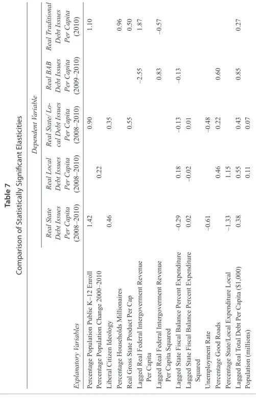
Tables 5 and 6 provide the regression results. Table 5 includes three sets of results for total borrowing in 2008, 2009, and 2010 (the 150 observation regressions) that use Real State Debt Issues Per Capita, Real Local Debt Issues Per Capita, and Real State/Local Debt Issues Per Capita as the dependent variables. Table 5 also includes a comparative regression using Real State/Local Debt Issues Per Capita from only 2008 and 2010 (100 observations) as the dependent variable. This compares 2008, a full year in which states could not issue Build America Bonds to 2010, a full year in which they could. In 2009, BABs were only issued after the month of April. We use the STATA statistical package and a random effects GLS estimation with heteroskedastic robust standard errors adjusted for clusters by each state to estimate these pooled sample regressions.16 We experimented with non-linearity in the relationships by taking the natural log of dependent variables, but found greater statistical significance through the inclusion of quadratic forms of explanatory variables when the simple linear form was statistically insignificant.17
Table 6 contains two sets of reduced form regression results (that use the single cross section data set with 50 observations) for the Real BAB Debt Issues Per Capita and Real Traditional Debt Issues Per Capita dependent variables. These regressions contain the same explanatory variables used in the full 150 data set regressions contained in Table 5 but allow us to see differences in the influences of these explanatory variables for BAB-specific issues and for traditional issues in 2010 when BABs existed as an alter-native form of debt financing that was not available in 2008 and 2009. In addition, in Table 6 we include a second Real BAB Debt Issues Per Capita regression that includes 15 Note that we also tried the specific ideological and political institution measures used by previous research to capture these political influences but never found any one measure (or group of measures) as statistically significant as this measure, which is widely used by political scientists to capture difference in liberal to political conservative ideology across the states.
16 Because we have explanatory variables that do not vary over the three 50 state cross-sections of data, we could not utilize a fixed effects estimation procedure. For comparison, we ran the Real State/Local Debt Issue Per Capita regression (recorded in column three of Table 5) using a fixed effects model that excluded all explanatory variables that did not vary over time. The only explanatory variables found significant were
Lagged Real Total Debt Per Capita and Lagged Real Federal Intergoverment Revenue Per Capita (with respective regression coefficients of 5.587 and –0.074).
17 We define statistical significance throughout this work as being at a 90 percent or greater confidence level using a two-tailed test.
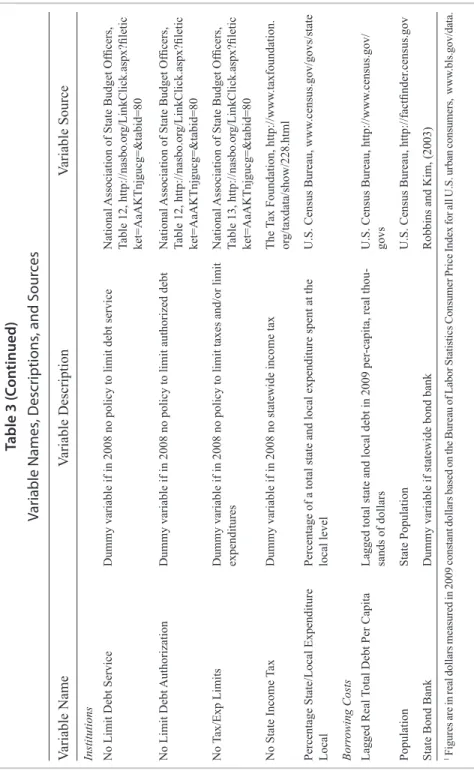
table 3 Var iable Names , D escr iptions , and S our ces Variable Name Variable Description Variable Source
Dependent Real State Debt Issues Per Capita
1
Higher education, state authority
, and state bond issue catego
-ries added together by state in 2009 per capita, real dollars for separate years 2008, 2009, and 2010
Personal correspondence with
Thomson Reuters
analyst
Real Local Debt Issues Per Capita
Local authority
, municipal, and county state bond issue catego
-ries added together by state in 2009 per capita real dollars for separate years 2008, 2009, and 2010
Personal correspondence with
Thomson Reuters
analyst
Real State/Local Debt Issues Per Capita Real State Debt Issues Per Capita plus Real Local Debt Issues Per Capita
Personal correspondence with
Thomson Reuters
analyst
Real BAB Debt Issues Per Capita
Build
America Bond Issues by state in 2009 per capita, real
dollars for partial year 2009 and full year 2010
The Bond Buyer
, www
.bondbuyer
.com
Real
Traditional Debt Issues Per
Capita
Real State/Local Debt Issues Per Capita in 2010 less Real BAB Debt Issues Per Capita
See above
BAB Debt Percentage of
Total Debt
Percentage of total state debt in 2010 that was issued in the form of Build
America Bonds
See above
State BAB Debt Percentage
All BAB
Debt
Percentage of all BAB Debt in the United States Issued by state in 2010
See above
Demographics Percentage Population Public K–12 Enroll Percentage of population enrolled in K–12 public schools for academic year
Digest of Education Statistics, www
.nces.ed.gov/
programs/digest
Percentage Population Change 2000–2010
Percentage change in population from 2000 to 2010
U.S. Census data, http://2010.census. gov/2010census and http://www
.census.gov/
Politics Liberal Citizen Ideology Revised 1960–2008 citizen ideology series measure developed by Berry
, et al. (1998 and 2010) for 2008; ranges from zero
(most conservative) to one (most liberal)
Personal correspondence with Richard Fording, political scientist at the University of Kentucky
.
Percentage Households Millionaires
Percentage of households whose wealth greater than one mil
-lion dollars
Phoenix Marketing International, http://www
.
phoenixmi.com/images/uploads/pdf_upload/ StateRankingsMillionaires20062010.pdf
Economics Real Gross State Product Per Cap
Gross state product in 2009 real dollars divided by Population
Bureau of Economic
Analysis, http://www
.bea.
gov/regional/gsp
Lagged Real Federal Inter
goverment
Revenue Per Capita
Previous fiscal year
’s federal revenue shared with state/local
governments in per
-capita 2009 real dollars
U.S. Census Bureau, www
.census.gov/govs/state
Lagged State Fiscal Balance as Per
-centage Expenditure
Previous fiscal year
’s end of fiscal year state government bud
-get balance as Percentage of state’
s expenditure
National
Association of State Budget Officers,
http://nasbo.or
g/Publications/FiscalSurvey
Unemployment Rate
Average yearly unemployment rate
Bureau of Labor Statistics, http://www
.bls.gov/
schedule/archives/laus_nr
.htm
Percentage Poor Roads
Percentage of state’
s arterial roads deemed in poor pavement
condition in 2007
American
Association of State Highway and
Transportation Officials, p. 10, http://roughroads. transportation.or
g/RoughRoads_FullReport.pdf
Percentage Good Roads
Percentage of state’
s roads deemed in good pavement condition
in 2007
American
Association of State Highway
and
Transportation Officials, p. 10, http://
roughroads.transportation.or
g/RoughRoads_
table 3 ( con tinued) Var iable Names , D escr iptions , and S our ces Variable Name Variable Description Variable Source
Institutions No Limit Debt Service
Dummy variable if in 2008 no policy to limit debt service
National
Association of State Budget Officers,
Table 12, http://nasbo.or
g/LinkClick.aspx?filetic
ket=AaAKTnjgucg=&tabid=80
No Limit Debt
Authorization
Dummy variable if in 2008 no policy to limit authorized debt
National
Association of State Budget Officers,
Table 12, http://nasbo.or
g/LinkClick.aspx?filetic
ket=AaAKTnjgucg=&tabid=80
No
Tax/Exp Limits
Dummy variable if in 2008 no policy to limit taxes and/or limit expenditures
National
Association of State Budget Officers,
Table 13, http://nasbo.or
g/LinkClick.aspx?filetic
ket=AaAKTnjgucg=&tabid=80
No State Income
Tax
Dummy variable if in 2008 no statewide income tax
The
Tax Foundation, http://www
.taxfoundation.
or
g/taxdata/show/228.html
Percentage State/Local Expenditure Local Percentage of a total state and local expenditure spent at the local level
U.S. Census Bureau, www
.census.gov/govs/state
Borr
owing Costs
Lagged Real
Total Debt Per Capita
Lagged total state and local debt in 2009 per
-capita, real thou
-sands of dollars
U.S. Census Bureau, http://www
.census.gov/
govs
Population
State Population
U.S. Census Bureau, http://factfinder
.census.gov
State Bond Bank
Dummy variable if statewide bond bank
Robbins and Kim, (2003)
1 Figures are in real dollars measured in 2009 constant dollars based on the Bureau of Labor Statistics Consumer Price Index for all U.S. urban consumers, www .bls.gov/data.
table 4
Variable Descriptive Statistics for 150 [50] Observation Regressions
Variable Name Mean DeviationStandard Minimum Maximum
Dependent
Real State Debt Issues Per Capita 607.94 409.74 0 2,202.93 Real Local Debt Issues Per Capita 402.25 271.16 0 1,642.51 Real State/Local Debt Issues Per Capita 1,003.09 500.89 53.19 3,841.08 Real BAB Debt Issues Per Capita [451.82] [307.82] [11.39] [1,005.69] Real Traditional Debt Issues Per Capita [2,471.36] [942.90] [232.61] [5,069.53] BAB Debt Percentage of Total Debt [2.00] [3.56] [0.007] [21.15] State BAB Debt Percentage All BAB Debt [14.66] [8.73] [0.399] [38.70]
Demographics
Percentage Population Public K–12 Enroll 15.98
[15.82] [1.53]1.44 [13.39]13.88 [21.58]21.63 Percentage Population Change 2000–2010 9.86
[9.86] [7.26]7.26 [–0.55]–0.55 [35.15]35.15
Politics
Liberal Citizen Ideology 61.34
[61.34] [17.55]17.55 [25.23]25.23 [91.85]91.85 Percentage Households Millionaires 4.55
[4.25] [0.97]0.97 [1.00]1.00 [6.41]7.12
Economics
Real Gross State Product Per Capita 42,900.82
[40,926.95] [7,915.42]8,921.26 [28,517.86]28,517.86 [62,604.44]74,545.06 Lagged Real Federal Intergoverment
Revenue Per Capita [1,671.61]1,697.06 [654.44]634.95 [933.15]933.15 [4,363.63]4,363.63 Lagged State Fiscal Balance as
Percentage Expenditure [9.13]11.46 [19.73]15.89 [–7.50]–7.50 [127.1]127.1
Unemployment Rate 7.49
[8.74] [2.05]2.38 [3.8]3.00 [13.7]13.7
Percentage Poor Roads 12.68
[12.68] [8.96]8.96 [0.00]0.00 [46.0]46.00
Percentage Good Roads 51.22
Real Traditional Debt Issues Per Capita as an additional explanatory variable. In this regression, we recognize that this explanatory variable is simultaneously determined. Thus, the use of two-stage least squares (2SLS) regression estimation requires finding instrumental variables expected to influence the offering of the newly included endog-enous variable in the regression, but not the dependent variable. We utilize the reason-able theory that a state’s subnational governments are more likely to offer traditional debt issues the greater the income tax benefits that residents in the state can potentially enjoy from purchasing these offerings. Benefits to a state’s residents come in the form of additional income tax deductibility in a state that has a higher rate of personal income taxation with a more progressive rate structure, with more high-income citizens who are more likely to pay the state’s income taxes, and does not tax interest earned by an individual on a municipal bond issued within the state.18 Under these circumstances, a
table 4 (continued)
Variable Descriptive Statistics for 150 [50] Observation Regressions
Variable Name Mean DeviationStandard Minimum Maximum
Institutions
No Limit Debt Service 0.36
[0.36] [0.40]0.48 [0]0 [1]1 No Limit Debt Authorization 0.10
[0.10] [0.30]0.30 [0]0 [1]1
No Tax/Exp Limits 0.38
[0.38] [0.49]0.49 [0]0 [1]1
No State Income Tax 0.18
[0.18] [0.39]0.39 [0]0 [1]1 Percentage State/Local Expenditure Local 50.20
[50.20] [9.37]9.31 [21.11]21.11 [66.56]66.45
Borrowing Costs
Lagged Real Total Debt Per Capita ($1,000) 76.88
[78.30] [26.91]25.42 [16.04]16.03 [148.95]150.15
Population (millions) 6.14
[6.18] [6.87]6.76 [0.57]0.53 [37.3]37.3
State Bond Bank 0.38
[0.38] [0.49]0.49 [0]0 [1]1
18 See Lovely and Wasylenko (1992) for evidence that states that exempt interest income on their own bonds for residents borrow at lower interest rates, due to the greater demand this creates to purchase these bonds.
table 5
Total Bond Issue Regression Results
(150 Observation Regressions: 2008, 2009, and 2010 Cross Sections of 50 States)
Dependent Variable Explanatory Variable Real State Debt Issues Per Capita Years 2008, 2009, and 2010 (Mean= $607.94) Real Local Debt Issues Per Capita Years 2008, 2009, and 2010 (Mean= $402.25) Real State/ Local Debt Issues Per Capita Years 2008, 2009, and 2010 (Mean= $1,003.09) Real State/ Local Debt Issues Per Capita Years 2008 and 2010 only (Mean= $977.80) Constant –110.62 (626.74) (557.61)–393.56 –1066.59***(638.83) –1,438.52***(631.36) Dummy 2009 259.49*** (85.20) (81.49)90.65 377.74***(134.19) NA Dummy 2010 194.76*** (74.81) 122.99***(57.58) 320.97***(98.01) 278.32***(103.79) Percentage Population Public
K–12 Enroll 53.96**(25.55) (21.66)–11.95 (31.21)56.71* (25.66)33.84 Percentage Population Change
2000–2010 (6.14)2.21 9.12**(4.27) (8.01)10.72 (6.21)5.30 Liberal Citizen Ideology 4.56*
(2.53) –0.642(1.85) 5.72***(2.33) 4.93**(2.47) Percentage Households
Mil-lionaires (54.53)8.83 (43.06)–14.33 (65.44)–18.79 (63.11)76.91 Real Gross State Product Per
Capita (0.008)0.011 (0.004)0.001 0.013**(0.006) 0.013**(0.007) Lagged Real Federal
Inter-goverment Revenue Per Cap (0.063)0.060 (0.049)–0.020 (0.076)0.074 (0.072)0.127* Lagged State Fiscal Balance as
Percentage Expenditure –15.26***(4.06) 6.28**(3.39) –11.14**(5.08) –5.49**(2.21) Lagged State Fiscal Balance
as Percentage Expenditure Squared 0.110*** (0.033) –0.049**(0.028) 0.076**(0.038) NA Unemployment Rate –49.77*** (19.94) (17.94)–7.47 –65.40**(27.38) (22.75)–20.13
table 5 (continued)
Total Bond Issue Regression Results
(150 Observation Regressions: 2008, 2009, and 2010 Cross Sections of 50 States)
Dependent Variable Explanatory Variable Real State Debt Issues Per Capita Years 2008, 2009, and 2010 (Mean= $607.94) Real Local Debt Issues Per Capita Years 2008, 2009, and 2010 (Mean= $402.25) Real State/ Local Debt Issues Per Capita Years 2008, 2009, and 2010 (Mean= $1,003.09) Real State/ Local Debt Issues Per Capita Years 2008 and 2010 only (Mean= $977.80) Percentage Poor Roads 1.47
(5.16) (3.52)4.33 (6.18)7.63 (5.42)1.28 Percentage Good Roads –0.693
(2.59) 3.65**(1.54) 4.32**(2.22) (2.22)2.11 No Limit Debt Service 43.70
(54.54) –83.11**(45.05) (70.41)–22.84 (48.97)–45.65 No Limit Debt Authorization –418.98***
(81.11) (60.06)–5.05 –415.92***(104.88) –265.51***(103.41) No Tax/Exp Limits –141.73***
(56.31) (52.61)–17.05 –165.68***(66.11) (48.41)–31.01 No State Income Tax –135.55*
(81.20) (70.01)–91.49 –226.86**(104.44) –130.81*(81.80) Percentage State/Local
Expen-diture Local –16.06***(4.85) 9.22***(3.63) (4.58)–3.99 (94.12)–2.14 Lagged Real Total Debt Per
Capita ($1,000) (1.57)2.98* 2.90**(1.42) 5.59***(1.97) 5.97***(1.53) Population (millions) 5.09
(6.12) (3.99)6.99* 11.31**(5.93) (4.94)8.29*
State Bond Bank –34.11
(60.74) (48.80)12.20 (73.08)–11.75 (57.46)–13.38
R-Squared 0.763 0.639 0.711 0.833
Note: Asterisks denote significance at the 90% (*), 95% (**), and 99% (***) confidence levels in a two-tailed test.
table 6
Build America Bond Regression Results
(50 Observation Regressions: 2010 Cross Section for 50 States) Dependent Variable Explanatory Variables Real Traditional Debt Issues Per Capita (Mean=$2,471.36) Real BAB Debt Issues Per Capita (Mean=$451.82) Real BAB Debt Issues Per Capita (Mean=$451.82) Constant –8,540.51** (2,404.51) (1,070.25)–501.24 (1,320.29)–212.75 Real Traditional Debt Issues
Per Capita (endogenous)1
NA NA 0.034
(0.101) Percentage Population Public
K–12 Enroll 171.21*(87.90) (44.30)59.11 (50.72)53.26 Percentage Population Change
2000–2010 (19.39)–12.46 (9.32)1.06 (9.53)1.49
Liberal Citizen Ideology 11.96
(8.88) (4.05)–1.29 (4.26)–1.70 Percentage Households Millionaires 556.33***
(156.38) (82.31)–23.52 (100.28)–42,55 Real Gross State Product Per Capita 0.029*
(0.017) 0.013**(0.006) (0.006)0.012* Lagged Real Federal Intergoverment
Revenue Per Capita 2.73***(0.803) –0.680**(0.314) –0.773*(0.395) Lagged Real Federal Intergoverment
Revenue Per Capita Squared –0.0005***(0.0001) 0.00013**(0.00006) 0.00015**(0.00007) Lagged State Fiscal Balance as
Percentage Expenditure (4.34)–5.73 –5.28**(2.37) –5.09**(2.51)
Unemployment Rate 23.82
(54.46) (27.34)–19.70 (27.67)–20.51 Percentage Poor Roads –14.32
(15.00) (7.54)10.45 (7.80)10.94
Percentage Good Roads 5.97
(5.40) (2.89)5.25* (2.76)5.04* No Limit Debt Service –146.87
(147.21) (77.89)–21.99 (81.96)–16.96 No Limit Debt Authorization –718.31*
table 6 (continued)
Build America Bond Regression Results
(50 Observation Regressions: 2010 Cross Section for 50 States) Dependent Variable Explanatory Variables Real Traditional Debt Issues Per Capita (Mean=$2,471.36) Real BAB Debt Issues Per Capita (Mean=$451.82) Real BAB Debt Issues Per Capita (Mean=$451.82) No Tax/Exp Limits –39.54 (172.45) (75.02)20.34 (77.03)21.69
No State Income Tax –147.44
(212.70) (137.80)–8.66 (139.25)3.62 Percentage State/Local Expenditure
Local (10.34)4.75 (6.55)–5.94 (6.60)–6.11
Lagged Real Total Debt Per Capita
($1,000) (4.29)8.84* 4.98**(2.17) (2.53)4.68*
Population (millions) 15.1
(12.2) (8.76)11.1 (8.76)10.6
State Bond Bank –147.12
(151.42) (83.13)65.62 (89.30)70.65
R-Squared 0.849 0.672 0.673
Note: Asterisks denote significance at the 90% (*), 95% (**), and 99% (***) confidence levels in a two-tailed test.
1 Instruments used and source: (1) Percent Households with Income 75K to 99K, (2) Percent Households with Income 100K to 124K, (3) Percent Households with Income 125K to 149K, (4) Percent Households with Income 150K to 199K, (5) Percent Households with Income 200K+ [all previous from U.S. Statistical Abstract, 2009, Money Income of Households, http://www.census.gov/compendia/statab/2009/cats/income_expenditures_ poverty_wealth/household_income.html ], (6) Highest Marginal Income Tax Rate and (7) Taxable Income Value that Highest Marginal Income Tax Paid [two previous from The Tax Foundation, 2009, State Individual Income Tax Rates, http://www.taxfoundation.org/taxdata/show/228.html], (8) State Taxes Own Municipal Bond Interest in Any Way dummy variable [http://www.investinginbonds.com/learnmore.asp?catid=5&subcatid=24&id=225], (9–13) No State Income Tax dummy variable multiplied by each household income category, (14–18) State Taxes Own Municipal Bond Issues in Any Way dummy variable multiplied by each household income category, and (19) a Rank variable that is set equal to one if Real Traditional Debt Issues Per Capita fall into the lowest 1/3 of values, two if the second 1/3 of values, and 3 if the highest 1/3 of values [as suggested by Krozsner and Stratman (2000) and Nguyen-Hoang (2012)]. The R-Squared on the first-stage regression that predicted Real Traditional Debt Issues Per Capita was 0.939.
An earlier version of this research only used the first eight instrumental variables. We followed a referee’s suggestion to add instruments used in other papers, and thus employ a first-stage estimation of Real Traditional Debt Issues Per Capita using 50 observations and 38 regressors.
state’s policymakers are likely to offer more traditional debt.19 This logic works well for satisfying the requirement that these instruments do not influence the dependent variable that measures a state’s offering of BABs because the interest earned on holding this form of debt by a state’s citizens does not enjoy such tax-free status. We assessed the appropriateness of this logic through the test of over-identifying instrumental variable restrictions as described in Wooldridge (2009), and found that we could not reject the null hypothesis that all of the 19 instruments (described in a footnote to Table 6) are exogenous to BAB issuance.20 Unfortunately, measurable and available exogenous fac-tors that drive a state’s issuance of BABs but do not influence the issuance of traditional debt are not apparent.21 Thus, we could not run the similar regression where Real BAB Debt Issues Per Capita explains Real Traditional Debt Issues Per Capita.
Consider first the explanatory factors found significant in the regression results recorded in Table 5 for all forms of long-term state/local debt issued in years 2008, 2009, and 2010, and compare these findings to the ones at the disaggregated state or local level. Based on the year dummies, holding other explanatory factors constant, in 2009 there was about $378 in more Real State/Local Debt Issues Per Capita issued than in 2008 and about $321 more in 2010 than in 2008. To place this in perspective, consider that the average real amount of this aggregate debt issue per capita was about $1,000 per year. Thus, holding other explanatory factors constant, subnational govern-ments in aggregate issued more long-term debt in the second year and third half year of the Great Recession than the first.22 Similar patterns emerged for separate state debt 19 Note that it would be theoretically reasonable to include some of these instrumental variables as explanatory variables in the previously run regressions. Such measures as Percentage Households with Income 75K to 99K, Percentage Households with Income 100K to 124K, Percentage Households with Income 125K to 149K, Percentage Households with Income 15Kk to 199K and Percentage Households with Income 200K
greater could all cause a state to offer more traditional debt if policymakers see it as tax free instrument for wealthy citizens in the state to take advantage of. When these variables were included, they were found statistically insignificant and also resulted in the loss of statistical significance for Real Gross State Product Per Capita. Given the high variance inflation factors calculated for these regressors, we decided that multicollinearity was likely to blame and dropped the income category measures.
20 This test involves estimating the 2SLS regression specified in column four in Table 6 and saving the calculated residuals. These residuals are then regressed against all exogenous explanatory variables in the model to obtain the R-squared (0.041) measure of fit of this regression. Finally, the value of R-squared is multiplied by 50 to yield 2.05. Since this value is less than the 27.2 test statistic derived from a Chi-Square distribution with q equal to 19 (number of instruments) and a 10 percent level of significance, with 90 percent confidence we cannot reject the null hypothesis of these being exogenous instruments.
21 The one possibility is to use a non-theory generated rank instrumental variable that is set equal to one if Real BAB Debt Issues Per Capita fall into the lowest 1/3 of values, two if the second 1/3 of values, and 3 if the highest 1/3 of values. We did not try this non-theoretical method of choosing an instrument for BABs but do utilize it as an additional instrument for predicting traditional debt.
22 Also relevant is the fact that municipal bond rates spiked in the last quarter of 2008, reflecting substantial uncertainty in financial markets. Indeed, non-taxable municipal rates exceeded Treasury bond rates for the first half of 2009 as a result of uncertainty and Fed action to reduce market rates. Municipal rates then declined substantially through 2009 and until the end of 2010, when they again spiked. Thus, part of the reason for increased municipal long-term bond issuance in 2009 and 2010 could be due to this fall in interest rate.
issues, whereas local debt issues were no different in 2009 and 2008, but were higher in 2010.
Very likely reflecting increased demand for public school infrastructure, the results in Table 5 indicate that a one percentage point increase in the percentage of a state’s population that attends a K–12 public school resulted in about a $57 per capita increase in state/local bond issues in a year and a very similar $54 per capita increase for this measure for the issuance of only state bonds. The only other demographic factor that influenced local debt issuance was the ten-year population change, with a 1 percent-age point rise in population resulting in about $9 more of annual local debt per person. Perhaps this is due to the more pressing need that local governments face to increase infrastructure after a population surge as compared to the state as a whole.
In the political realm, Table 5 documents that more liberal states issued both more state debt and more aggregate state/local debt per capita, with increases of about $5 and $6 in each category for every one point increase in the zero (very conservative) to 100 (very liberal) scale used. Our regression findings indicate a positive relationship between Gross State Product per capita and per capita bond issues for state-local governments together. Very interestingly, as the fiscal surplus enjoyed by a state government rose, states issued less (at an increasing rate) Real State Debt Issues Per Capita, while locali-ties issued more (at a decreasing rate). The influence detected for aggregate state/local debt mimicked the state-only influence. A higher statewide unemployment rate of one percentage point exerted depressing influences on state debt issues per capita of about $50, and on state/local debt issues of about $65. A higher Percentage Good Roads caused states to issue more debt to maintain that status, as expected.23 The result suggests that about a one percentage point change in good roads lead to an expected $4 increase in
Real Local Debt Issues Per Capita and aggregated state/local debt issues. Perhaps it is a telling commentary on the causes of the declining quality of public infrastructure in many states that while states with more good roads issue more debt, the existence of more poor roads exerts no influence on debt issue.
The results in Table 5 also exhibit the influence of statewide institutional factors on debt issue. If a state did not restrict in any way the payment of its interest on state issued debt, local governments offered about $83 less debt per capita relative to a mean offering of $402. No limit on state debt authorization resulted in states offering $419 less in state debt per capita (relative to a mean offering of $608) and $416 less in state/local debt per capita (relative to a mean offering of $1,003). Perhaps this indicates that states with inherent difficulty in controlling their debt issues in the past (since these measures were all at least adopted a decade earlier) are more likely to adopt limitations. Interestingly, states without a limitation on their level of taxation and/or spending were less likely 23 One could argue that good roads (as measured here by pavement quality) in a state are a result of routine maintenance that is not financed through borrowing. But given the age of the roadway infrastructure in most states, maintaining a high percentage of roads in a state classified as “good” likely requires much replacement activity and hence the use of debt to finance it. Road quality also may serve as a proxy for public capital depreciation.
to issue state debt ($142 less) and state/local debt ($166 less). This may indicate that a constraint on funding additional state government activity with current revenue pushes the state in the direction of using more bond financing. States without an income tax are also likely to issue $136 less in annual state debt issue and $227 less in state/local debt issue. We suspect that this reflects a sentiment in the state for less government activity and hence a smaller need for bond financing. The institutional factor of Percentage State/Local Expenditure Local is serving its purpose of controlling for differences in the division of subnational activity in states by showing that for every one-percentage point increase in this measure local debt rose by $9 and state debt fell by $16.
Furthermore, the results offered in Table 5 indicate that for every thousand-dollar increase in the previous year’s per capita debt, both state governments and local govern-ments were likely to issue about $3 more in current year’s debt, resulting in an aggregate state/local finding of a $6 increase per $1,000 higher in Lagged Real Total Debt Per Capita. Local governments in states with greater population also offered more Real Local Debt Issues Per Capita of $7 per every million increase in the state’s popula-tion. An $11 aggregate increase in state/local debt also resulted from a million person increase in state population. Unlike previous empirical work, we find no evidence that the presence of a state bond bank influenced the issue of long-term subnational debt during the Great Recession.
The regression results in the last column of Table 5 use the dependent variable of
Real State/Local Debt Issues Per Capita for only the years 2008 and 2010. Statistically significant regression coefficients exhibit the same signs as found in the same table for all three years. The positive and significant coefficient on Dummy 2010 indicates that in the year that BABs were fully available (2010), in comparison to the year that they were not (2008), states on average issued about $278 more in debt issues per person (given a mean issue of about $978).24 This comparison of only 2010 to 2008 further supports the hypothesis that the ability to offer BABs stimulated, as was intended, greater borrowing by states.
Turning now to Table 6, the results demonstrate that the percentage of a state’s population that is enrolled in K–12 public schools still exerts a positive influence on traditional debt issues in 2010 alone but exerts no statistically significant influence on BAB issues. Unlike the findings for 2008 through 2010, we find that a one percentage point increase in the percentage of households that are millionaires raises traditional debt issues by $556 (on a mean of $2,417), but had no influence on BAB issues. Why states with this higher presence of upper-end affluence were more likely to use tradi-tional debt, but not BAB debt (when they had a choice between BABs or traditradi-tional, but not when they did not have a choice), is not entirely clear. One possibility is that greater affluence in a state encourages its policymakers to issue more traditional debt (that if purchased by these wealthy citizens extends a state and federal income tax 24 As noted earlier, the 30-year yield on Treasury Bills was very similar in both of the years, so the influence