AN INTEGRATED, MODULE-BASED BIOMARKER DISCOVERY FRAMEWORK
by
Grace T. Huang
B.S., Cornell University, 2004
Submitted to the Graduate Faculty of School of Medicine in partial fulfillment
of the requirements for the degree of Doctor of Philosophy
University of Pittsburgh 2013
UNIVERSITY OF PITTSBURGH SCHOOL OF MEDICINE
This dissertation was presented by
Grace T. Huang
It was defended on September 30, 2013
and approved by
Takis V. Benos*, Ph.D. Dept. of Computational Biology, University of Pittsburgh Chakra S. Chennubhotla, Ph.D. Dept. of Computational Biology, University of Pittsburgh
Ziv Bar-Joseph, Ph.D. School of Computer Science, Carnegie Mellon University Naftali Kaminski, M.D. School of Medicine, Yale University
Ioannis Tsamardinos, Ph.D. Dept. of Computer Science, University of Crete Thesis Director: Gregory F. Cooper, M.D. Ph.D. Dept. of Biomedical Informatics,
Copyright © by Grace T. Huang 2013
Identification of biomarkers that contribute to complex human disorders is a principal and challenging task in computational biology. Prognostic biomarkers are useful for risk assessment of disease progression and patient stratification. Since treatment plans often hinge on patient stratification, better disease subtyping has the potential to significantly improve survival for patients. Additionally, a thorough understanding of the roles of biomarkers in cancer pathways facilitates insights into complex disease formation, and provides potential druggable targets in the pathways.
Many statistical methods have been applied toward biomarker discovery, often combining feature selection with classification methods. Traditional approaches are mainly concerned with statistical significance and fail to consider the clinical relevance of the selected biomarkers. Two additional problems impede meaningful biomarker discovery: gene multiplicity (several maximally predictive solutions exist) and instability (inconsistent gene sets from different experiments or cross validation runs).
Motivated by a need for more biologically informed, stable biomarker discovery method, I introduce an integrated module-based biomarker discovery framework for analyzing high-throughput genomic disease data. The proposed framework addresses the aforementioned challenges in three components. First, a recursive spectral clustering algorithm specifically
AN INTEGRATED, MODULE-BASED BIOMARKER DISCOVERY FRAMEWORK
Grace T. Huang University of Pittsburgh, 2013
tailored toward high-dimensional, heterogeneous data (ReKS) is developed to partition genes into clusters that are treated as single entities for subsequent analysis. Next, the problems of gene multiplicity and instability are addressed through a group variable selection algorithm (T-ReCS) based on local causal discovery methods. Guided by the tree-like partition created from the clustering algorithm, this algorithm selects gene clusters that are predictive of a clinical outcome. We demonstrate that the group feature selection method facilitate the discovery of biologically relevant genes through their association with a statistically predictive driver. Finally, we elucidate the biological relevance of the biomarkers by leveraging available prior information to identify regulatory relationships between genes and between clusters, and deliver the information in the form of a user-friendly web server, mirConnX.
TABLE OF CONTENTS
1.0 Introduction ... 14
1.1 Personalized medecine and biomarker discovery ... 14
1.2 Biological background ... 17
1.2.1 Gene expression and microarray ... 17
1.2.2 Transcriptional regulation ... 19
1.2.3 Post-‐transcriptional regulation ... 20
1.3 Limitations of current biomarker discovery methods ... 22
1.4 Motivating example ... 26
1.5 Outline of our approach ... 29
1.6 Contributions ... 31
1.7 Overview and organization ... 33
2.0 ReKS: Recursive K-‐means Spectral Clustering ... 34
2.1 Clustering overview and motivating example ... 35
2.2 Spectral clustering ... 37
2.3 Method overview ... 40
2.4 Performance evaluation ... 42
2.4.1 Comparison to other methods on TCGA cancer data ... 42
2.4.1.1 Data description ... 42
2.4.1.3 Cluster quality evaluation ... 45
2.4.2 Benchmarking against patient data ... 47
2.5 Prior incorporation ... 49
2.6 Improving ReKS stability using eigencuts ... 52
2.7 Discussion and future directions ... 55
3.0 T-‐ReCS: Tree-‐guided cluster selection ... 57
3.1 Variable selection methods ... 59
3.1.1 Traditional variable selection methods ... 59
3.1.2 Efforts toward stable, non-‐redundant, or group feature selection ... 60
3.2 Local causal induction ... 62
3.2.1 Bayesian networks ... 62
3.2.2 Feature selection as a Bayesian network structure learning problem ... 65
3.2.3 Local structure learning ... 67
3.2.4 Skeleton identification methods ... 68
3.2.5 Max-‐Min Parent Children (MMPC) ... 70
3.3 Tree-‐guided Cluster Selection (T-‐ReCS) ... 75
3.3.1 Method overview ... 75
3.3.2 Tests of conditional independence ... 81
3.3.2.1 Conditional independence tests employed by single variable MMPC ... 82
3.3.2.2 Conditional independence tests employed by T-‐ReCS ... 84
3.3.3 Choosing latent variable representation ... 86
3.3.3.1 Centroid ... 86
3.3.3.2 Medoid ... 87
3.3.3.3 Principle Component Analysis (PCA) ... 87
3.4.1 Accuracy ... 89
3.4.1.1 Continuous data, categorical target variable : SVM and AUC ... 89
3.4.1.2 Continuous data, censored survival target variable: Cox regression and CI . 90 3.4.2 Stability ... 93
3.4.3 Cluster Size ... 94
3.4.4 Choosing suitable parameters: cross validation ... 94
3.5 Results ... 94
3.5.1 Simulated data and results ... 95
3.5.2 Application: Melanoma gene and miRNA expression ... 104
3.6 Discussion and future directions ... 106
4.0 mirconnx: condition-‐specific mRNA-‐miRNA network integrator .. 110
4.1 Motivation ... 111
4.2 Method overview ... 112
4.2.1 Method overview ... 112
4.2.2 Building a prior network ... 115
4.2.2.1 TF to gene/miRNA regulations ... 115
4.2.2.2 miRNA to gene/TF regulations ... 116
4.2.2.3 Gene expression preprocessing ... 116
4.2.2.4 Constructing association network from gene expression data ... 117
4.2.3 Network integration ... 118
4.3 User interface ... 119
4.3.1 Input format ... 119
4.3.1.1 Submission and waiting time ... 119
4.3.1.2 mirConnX output ... 120
4.4 Application: TCGA ... 122
4.6 Discussion and future directions ... 127 5.0 Conclusion ... 129 5.1 Concluding remarks ... 129 5.2 Future directions ... 131 APPENDIX A ... 133 APPENDIX B ... 135 APPENDIX C ... 137 APPENDIX D ... 139 bibliography ... 141
LIST OF TABLES
Table 1.1 A list of commercially available molecular diagnostic tests ... 17 Table 1.2 Tumor-associated microRNAs and their validated target genes[51] ... 22 Table 1.3 A list of candidate genes that define Basal versus Luminal breast cancer subtypes. ... 27 Table 2.1 ReKS average execution time compared to other methods ... 47 Table 3.1 A list of benchmarking datasets used in this evaluation ... 104
LIST OF FIGURES
Figure 1.1 Illustration of a two-color microarray experiment ... 19
Figure 1.2 An example of gene multiplicity and its implications………..28
Figure 1.3 Overall approach of the proposed module-based biomarker discovery framework .... 31
Figure 2.1 Clustering patient data is more difficult than cell-based data. ... 37
Figure 2.2 Demonstration of the ReKS method on the GBM dataset. ... 41
Figure 2.3 Distribution of cluster sizes produced by ReKS and by other methods ... 44
Figure 2.4 Performance of ReKS compared to other methods………...………..46
Figure 2.5 Benchmarking ReKS on patient data. ... 49
Figure 2.6 ReKS with prior incorporation applied on BRCA dataset. ... 51
Figure 2.7 Detailed look of BRCA results. ... 52
Figure 2.8 An example of the EigenCuts algorithm. ... 54
Figure 2.9 An example of EigenCuts performance across two parameters. ... 55
Figure 3.1 Illustrations of a Bayesian Network and Markov Blanket……….…...…...64
Figure 3.2 The Max-Min Parents and Children (MMPC) Algorithm ... 72
Figure 3.3 An example to illustrate the selection procedure of T-ReCS. ... 78
Figure 3.5 An order graph for Concordance Index calculation and bipartite maximum weight
matching for cluster stability calculation. ... 92
Figure 3.6 A simulated linear Gaussian Bayesian network. ... 96
Figure 3.7 Variables selected by T-ReKS over cross validation. ... 98
Figure 3.8 An example of the ReKS tree on simulated data. ... 101
Figure 3.9 T-ReCS performance on simulated data. ... 103
Figure 4.1 Overview of the integrated analysis in mirConnX………...………..114
Figure 4.2 Snapshot of the glioblastoma case study output. ... 121
PREFACE
I am indebted to many whose help made this dissertation possible.
First and foremost, I am sincerely grateful for the guidance and support of my thesis advisor, Dr. Takis Benos. His encouragements and mentorship throughout the years had helped me grow into who I am today. I deeply appreciate Dr. Chakra Chennubhotla, for the numerous stimulating discussions we had that evolved into an integral part of this work, and whose enthusiasm inspires me greatly. I am also hugely grateful for the guidance of Dr. Ioannis Tsamardinos. A conversation with him some years back led to the conception of this work, and the fruitful discussions throughout the years shaped the work into what it is today. In addition, without the critical comments and feedback of the rest of my committee members Dr. Greg Cooper, Dr. Ziv Bar-Joseph, and Dr. Naftali Kaminski, this dissertation would not be complete.
I would like to thank Dr. Abha Bais and Dr. Seyoung Kim for helpful discussions and mentorship, Harry for all his technical support, and all the rest of the past and current Benos lab members: Rachel, Sabah, Claudia, AJ, and Kristina, for discussions and critiques. I would like to also thank all the individuals in the Kaminski lab, the Tawbi lab, the Tseng lab, the TCGA group, and the CMPI group with whom I have had the pleasure to collaborate with along the way. I am thankful for the friendship of Justin, John, Cordelia, Anindita, Virginia, Andrej, Jacob, Luis, Ming, Guy and Marcel and many more, whose love and support helped carry me through. Finally, this work would not be possible without the love and support of my family.
1.0 INTRODUCTION
1.1 PERSONALIZED MEDECINE AND BIOMARKER DISCOVERY
Human diseases such as cancer have been shown to be complex and heterogeneous [1]. They often exhibit diverse morphologies, molecular characteristics, and clinical properties. Traditionally, a uniform drug regimen is administered to patients displaying similar pathology. However, these patients often vary in clinical outcome and responsiveness to drug therapy. This one-size-fits-all approach is suboptimal and often ineffective. As such, the biomedical community has recognized the need for individualized therapy, and considerable research effort have been directed toward the development of personalized medicine.
Personalized medicine holds one of the greatest promises of modern clinical medicine. The term is coined for customized medical decisions or drug products tailored for individual patients, often based on emerging technology or diagnostic tools not previously available. In reality, personalized medicine is still at its infancy. Treatment plans are not yet routinely devised at the granularity of individual patients, but instead at the level of patient cohorts. Since proper selection of treatment plans hinges on definition of patient cohorts, accurate diagnosis and patient stratification has the potential to significantly improve patient outcome, survival, and quality of life [2].
Disease diagnosis and subtyping can be achieved by detecting the presence or abundance of biomarkers. We define a biomarker to be an entity that can be measured to provide actionable
information regarding biological processes, disease progression, or responses to therapeutic intervention. Additionally, biomarkers can be used to measure progress and therapeutic response of disease after a treatment plan [3]. An ideal biomarker is one that is present or absent only in diseased patients versus healthy controls, or one whose relative abundance differ among subtypes of diseases.
Identifying such biomarkers for complex human disorders is a principal and challenging task. Not only are prognostic biomarkers useful in assessing risk of disease progression and stratifying patients, a thorough understanding of the roles of biomarkers in cancer pathways facilitates insights into complex disease formation, and provides potential druggable targets in the pathways. The latter is especially crucial, as progress has yet to be achieved in improving survival for several common cancers such as lung or colon cancers. Thus, novel therapeutic strategies based on a deeper understanding of the cellular and molecular mechanisms of disease formation are urgently needed [1].
An example of a traditional biomarker for complex human disease is immunohistochemical (IHC) panel including estrogen receptor (ER), progesterone receptor (PR), and human epidermal growth factor receptor 2 (HERs). This set of single biomarkers has been used for several years in various aspects of breast cancer management. The presence of absence of these markers identifies three main subtypes [4]: luminal (ER+ and/or PR+), HER2-like (mainly ER- and HER2+), and basal-like (ER-, PR-, HER2, or triple-negative described by Schneider et al.[5]. They vary in their prevalence and prognosis, with triple negative patients facing the worst prognosis. These biomarkers have enabled physicians to make informative decision on cancer treatment. However, the prognostic ability of these markers is not ideal and difficulties still exist in stratifying subtypes of patients [6].
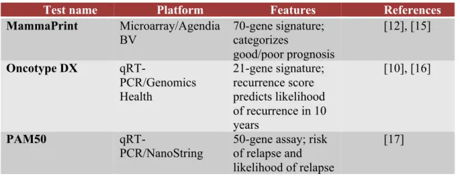
Possibilities of novel biomarkers have been proposed in light of the advance of microarray, sequencing technologies, and mass spectrometry technologies. These new high-throughput genomic technologies have facilitated the identification of –omics based biomarkers such as gene expression profiles or molecular signatures composed of several dozen to several thousand genes [7]–[9], several of which have been made commercially available (Table 1.1). In one of the pioneering studies, a molecular signature among breast cancer patients was used to predict recurrence of cancer after surgery with significant accuracy[10]. This diagnostic test is helpful in guiding the decision of whether the patients require continuing chemotherapy. A very recent study [11] also demonstrated the potential of molecular subtyping to guide therapy in early-stage, invasive breast cancer. In this study, Gluck and colleagues performed molecular subtyping of early-stage breast cancer with the MammaPrint [12] and BluePrint [13] tests to identify a group of patients, Luminal A, who do not benefit from neoadjuvant (preoperative) chemotherapy and show a high five-year metastases-free survival rate. This group could not be identified using traditional clinical tests such as immunohistochemistry and fluorescence in situ hybridization (IHC/FISH). We list some of the current commercially available molecular diagnostic tests in Table 1.1. The 70-gene assay (MammaPrint, Agendia, Netherlands) and the 21-gene assay (Oncotype DX, Genomic Health, USA) are the most widely used breast cancer multigene classifier assays. A 50-gene assay (PAM50, NanoString, USA) has also shown promise. Excellent summaries and review can be found in [14].
Encouraged by the recent success of molecular diagnostics, we developed a molecular biomarker discovery framework that could be used as the first step toward disease subtyping. In the next sections, I provide the biological background necessary for further discussion, including the measurements and regulation of gene expression.
Table 1.1 A list of commercially available molecular diagnostic tests
Test name Platform Features References
MammaPrint Microarray/Agendia BV 70-gene signature; categorizes good/poor prognosis [12], [15] Oncotype DX qRT-PCR/Genomics Health 21-gene signature; recurrence score predicts likelihood of recurrence in 10 years [10], [16] PAM50
qRT-PCR/NanoString 50-gene assay; risk of relapse and likelihood of relapse
[17]
1.2 BIOLOGICAL BACKGROUND
1.2.1 Gene expression and microarray
The abundance of mRNA products is called gene expression. Gene expression measurement is a popular and cheap way to infer the state of cells under a given condition. A genome wide measurement of transcription is called an expression profile and reflects the transcription level of the genes in the particular condition in which they are extracted from. While in general the gene expression measurement is directly correlated with the level at which the genes are being transcribed, they do not reflect other aspects of the biological processes such as protein levels and their activity. However, mRNA levels are easier to measure than protein levels, thus we use gene expression level as a reasonable substitute. As mentioned in the previous section, the availability of microarray technology has also enabled the search for molecular biomarkers.
In the last two decades, technical advances have lead to development of gene expression microarrays. Expression microarrays have enabled researchers to measure the abundance of
thousands of mRNA targets simultaneously [18], [19], providing a genomic, holistic view of gene expression. Microarray technology is based on hybridization: a process in which a strand binds to its unique complementary strand. On a microarray, a set of probes is attached to a solid surface (chip). A sample containing fluorescently tagged sequences are allowed to interact with the probes, and based on intensity of the fluorescence, the (relative) abundance of the targets of interests can be determined. There are two broad categories of microarrays: two-channel and single channel. Two-channel microarrays allow two individually labeled samples to hybridize competitively on the same surface to determine the relative abundance of the genes between the two samples. In contrast, one-color microarray only one sample is used. An illustration of the two-channel microarray is shown in Figure 1.1.
The biomedical community has witnessed an exponential growth in gene expression profiled from clinical samples, and several large consortiums [20]–[22] in addition to the Gene Expression Omnibus(GEO)[23] have systematically collected gene expression measurements from patients. Clinical gene expression data that we work with in this dissertation are generally extracted from biopsies of tumor samples and healthy tissues taken from patients or volunteers that participate in the studies. The gene expression profiles are typically measured on the same platforms across samples and common pre-processing steps including background correction, imputation, and normalization are performed together.
Gene expression is a tightly regulated process. The expression of a given gene at any given time depends on a complicated series of feedback and regulation that are controlled by many factors, including chromatin states, methylation status, transcription factor binding and suppression by a family of small RNAs. In the next sections, we focus on the last two types of regulation.
Figure 1.1 Illustration of a two-color microarray experiment http://upload.wikimedia.org/wikipedia/en/c/c8/Microarray-schema.jpg
1.2.2 Transcriptional regulation
In transcriptional regulation, proteins known as transcription factors (TFs) are recruited by a set of protein complexes and Pol II [24] to bind a promoter region of protein coding genes to either initiate(activators) or block(repressors) the activation of the gene. The core promoter region
typically consists of several hundred base pairs surrounding the transcription start site of a gene, and encompass a wide range of characteristics such as the presence of CpG islands, TATA box, methylation, and various other sequence elements [25], [26]. The regulatory region outside of the core promoter can be bound by TFs that typically contain a DNA binding domain that binds to specific set of sequence motifs 6-15bp in length [27]. There are over 2000 TFs that can be organized into families based on their structural properties and corresponding binding motifs [28], [29]. The TF can regulate its targets alone, in conjunction with other co-regulators, or in competition [30]. Identification of transcription factor bindings sites (TFBS) has been a major topic of interests for many years in the computational biology community. The short and degenerate nature of the motifs makes it a challenging task to identify them in the genomic region. Nevertheless, a number of tools and publications have resulted, often taking advantage of information such as conservation across species, presence in promoters of co-regulated genes, in addition to sequence specificity [31]–[33]. Several databases additionally contain curated experimental information that further supports the regulatory relationships of TFs and targets [34]–[36].
TFs are known to participate in cancer and disease formation. A large number of transcription factors involved in cell differentiation and apoptosis have been identified over the years [37]–[40], perhaps most famous of which is p53 [41], a tumor-suppressor gene, whose inactivation is one of the key hallmarks of a tumor.
1.2.3 Post-transcriptional regulation
First identified in 1993 by Lee et al. [42], microRNAs(miRNAs) are small (20-23 nt), non-coding single stranded RNA molecules that play an important role in post-transcriptional
regulation of protein-coding genes. The regulations are post-transcriptional, as their regulatory event occurs after mRNAs have been transcribed, by binding to the target sites of the 3’untranslated regions of protein coding genes. miRNAs are believed to be mostly transcribed by RNA Polymerase II [43] and less frequently, RNA Polymerase III [44]. The initial full-length miRNA forms a hairpin structure, which is then processed by two proteins, Drosha and Dicer, to form the final ~22nt product associated with a protein complex containing Argonaut. The miRNAs bind to the target sites on the 3’UTRs of target genes through base complementarity [45]. This binding can either lead to full degradation of the target mRNA transcript, or the blocking of its translation. Exact mechanisms for both are still under investigation, and current evidence seems to support both forms of suppression. Each miRNA can target many mRNAs, and each mRNA can in turn be the targets of multiple miRNAs [46].
Many miRNA target prediction algorithms have been developed [47]–[49]. In general, they combine sequence information, energy calculations, and various sequence contextual information such as position and nucleotide compositions, as well as conservation across species to infer possible binding sites of a given miRNA. A comprehensive review and discussion of various target prediction methods can be found in [50].
miRNAs have been found in all animal lineages, and have been implicated as critical regulators during disease formation and tumorgenesis [51]. In this dissertation, we are interested in both the abundance of miRNAs in disease samples, as well as the target genes and potential oncogenes that they regulate. There is mounting evidence that miRNAs can be useful for cancer prognosis. miRNA expression profiles for different tumor subtypes are unique due to tissue specificity. Using miRNA profiles, Lu et al. were able to correctly classify 12 of 17 poorly
differentiated carcinomas [52]. The Table 1.2 highlights some of the miRNAs and targets found to be associated with tumors.
Table 1.2 Tumor-associated microRNAs and their validated target genes [51]
NSCLC: Non-small cell lung cancer; CLL: chronic lymphocytic leukemia; GBM:Glioblastoma multiforme.
miRs Tumor Type Expression Target Genes
let-7 NSCLC Down RAS
miR-15a,miR-16 CLL Down BCL2 miR17-92 polycistron Breast, B-cell lymphomas Up AIB1,E2F1,TGFBR2,Tspi,CTGF miR-21 Breast, GBM Up TPM1
miR-106a Colon, pancreas, prostate Up TPM1
miR-221-222,miR-146b
Tyroid, papillary Up KIT
miR-372-373 Testis, germ cell tumors Up LATS2
Having introduced the motivation behind biomarker discovery and associated introductory concepts in biology, we now turn to the computational aspects of biomarker discovery and discuss some of its current limitations.
1.3 LIMITATIONS OF CURRENT BIOMARKER DISCOVERY METHODS
We aim to develop biomarker discovery methods that could be used as the first step toward disease subtyping. From a statistical perspective, biomarker discovery can be best cast as a variable selection problem, and identification of cancer subtype can be viewed as the associated classification step. The variables under selection are the molecular attributes of interest, in our case genes, genetic variations, or metabolites; the observations are samples from which the variables are measured e.g. patients. The goal is to search for the most discriminating features with respect to the labels for the observations.
Aside from its usefulness in extracting biological information, variable selection is critical in our application from a computational perspective. High-throughput genomics data is high dimensional, often with tens of thousands of variables measured simultaneously. However, the sample size is severely limited compared to the size of the variables. This is known as a phenomenon called curse-of-dimensionality [53], where the dimension of the variable space increases so fast that the available data becomes extremely sparse in this space. This sparsity is problematic for many methods that require statistical significance [54], [55]. Dimensionality reduction methods or variable selection are often performed as the first steps in analysis of omics data.
Many variable selection methods have been applied toward biomarker discovery using omics data. A review of the existing variable selection methods can be found in Section 3.1.
Even though numerous computational methods have been proposed for this purpose, clinical adoption of these biomarker discovery methods have been slow and limited due to a lack of reproducibility of the results. We detail several computational challenges and sources of non-reproducibility in biomarker discovery for omics data.
• Heterogeneity
Cancer is highly heterogeneous with respect to molecular alterations, cellular compositions, and clinical outcome [56]. This creates a principal challenge in biomarker discovery. Individual tumors are defined by distinct molecular changes and mechanisms. Further complicating the picture is the fact that tumors have a complex tissue structure comprised of malignant cells, tumor stromal components, host cells, and adjacent normal tissues. This molecular heterogeneity, along with the complex micro environment in which the tumor resides, makes analysis of high-throughput measurements taken from pooled samples of tumor a very challenging task.
Statistically, heterogeneity presents us with the problem of high level of noise. For example, we may not see perfect differential expression between normal tissues or patient samples, even if stratified with the most discriminative predictor.
• Multicollinearity (correlation)
Another intricate challenge in omics data variable selection is that cellular processes are often coupled and synchronized due to internal cellular regulation or external signals and stimulations. Variables of interest can display similar behavior. For example, many genes regulated by the same activator/repressor or whose protein products physically interacting with each other would display similar expression patterns across different conditions or across time points. This results in a correlation structure among the variables. This correlation structure would break down the assumptions of a lot of traditional variable selection methods designed for uncorrelated data [57], rendering them unsuitable for the task of biomarker discovery.
• Multiplicity and Instability
Two other problems that impede meaningful biomarker discovery are: gene multiplicity and instability. Gene multiplicity alludes to the fact that several maximally predictive solutions (gene sets) can co-exist [58], [59]. This may be due to the multicollinearity problem alluded to previously, but coexisting maximally predictive solutions may not necessarily be correlated. Instability refers to the phenomenon that inconsistent gene sets are selected from different research groups, different experiments conducted in the same lab, or even among different subsets of the data [60]. Many existing variable selection algorithms are designed with no regard to stability, as they seek to optimize only the predictive performance. These two issues are tightly coupled with the problem of multicollinearity, heterogeneity, and the high dimension of the data relative to sample size, and are possibly the main contributors to a lack of
reproducibility in biomarker discovery.
In addition to these computational challenges, two additional properties are often overlooked by biomarker discovery methods developed from a purely computational perspective:
• Network context
In recent years, the systems biology community has shifted toward a network-centric view on pathogenesis. It has become widely accepted that pathways rather than individual genes dictate the course of carcinogenesis and complex human disease formation [61]. Different mutations in the same pathway can all result in dysregulation, such as excessive cell proliferation, which forms the basis of tumor growth [62], [63]. This fact unfortunately implies that the traditional paradigm that relies on features being over-represented in disease samples would fail to recognize biomarkers that are only present in subsets of the disease samples.
• Clinical relevance
In addition, traditional approaches are mainly concerned with statistical significance and often neglect to consider the clinical relevance of the selected biomarkers. While they have been applied to the problem of biomarker discovery to varying degree of success, they are usually done to optimize toward statistical significance without considering biological importance of the features. As a result, a gene with no biological relevance to the specific target variable may be selected simply because its expression pattern is similar to the expression pattern of truly important genes (multiplicity) and running the same algorithm on different sets of data could result in discrepancy in genes selected (instability).
1.4 MOTIVATING EXAMPLE
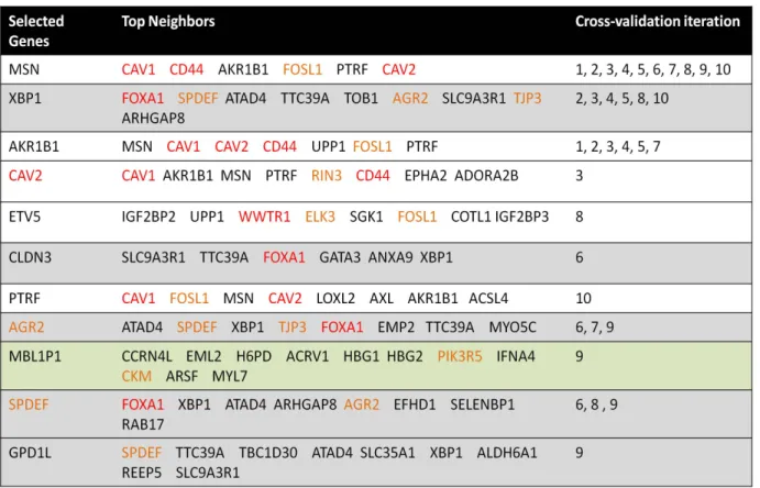
We provide an example (Table 1.3 and Figure 1.2) to illustrate some of the challenges alluded to in the pervious section. In this breast cancer gene expression data, we are interested in identifying genes that differentiate the two cancer subtypes: Basal (24 samples) and Luminal (36 samples). In 10-fold cross validation, a total of 11 candidate genes are selected by a feature selection method (HITON-PC [64]). The top candidate gene, MSN, is consistently selected in all cross-validation iterations (Table 1.3), yet it does not seem to directly play a role in tumor growth. When we examine its closest neighbors (genes) in terms of similarity in expression across the samples, we observe that several are indeed tumor suppressors (CAV1, CAV2, CD44). Similarly, XBP1 is selected in several rounds. While it is not directly known to be involved with breast cancer, its closest neighbor FOXA1 is known to be involved in ESR-mediated transcription in breast cancer cells (Figure 1.2). Interestingly, when we examined the local potential regulatory relationships between the selected genes and their top neighbors, we found potential XBP1 transcription factor binding sites in the promoter of FOXA1 (Figure 1.2). This observation suggests that a method that performs variable selection on groups of variables and additionally provides contextual information around the selected groups could provide more biologically robust and meaningful biomarkers.
Table 1.3 A list of candidate genes that define Basal versus Luminal breast cancer subtypes. Marked in red are genes known to be involved with tumorgenesis. Marked in orange are genes known to have potential roles in tumor growth and energetic. Rows highlighted in the same color are gene groups that cluster
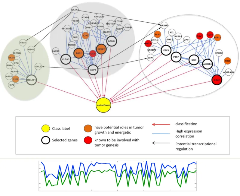
Figure 1.2 An example of gene multiplicity and its implications.
(Top) Selected candidate genes and their top neighbors placed in context of regulatory network. Genes in bold borders with a red arrow pointing to the class label (Luminal/Basal, yellow node) are those selected, as shown in Table1.3. Their top neighbors with expression highly correlated to theirs are connected to them in blue edges. Black arrows indicate potential regulatory relationships based on presence of binding motifs in promoters. Orange and red coloring of the nodes indicate their potential role in tumor genesis, consistent with color scheme Table 1.3. Finally, the grouping of the nodes and their respective background colors indicate potential clusters, consistent with color scheme in Table 1.3. (Bottom) Expression levels of XBP1 (blue) and FOXA1 (green) are plotted across samples. XBP1 and FOXA1 have very similar expression patterns, but XBP1 is chosen as the candidate gene.
1.5 OUTLINE OF OUR APPROACH
This dissertation illustrates my attempt to address each of these issues in the form of a three-component, module-based biomarker discovery framework.
We conjecture that due to the complex nature of pathogenesis, several sets of molecular signatures could be equally predictive of disease state. Furthermore, we hypothesize that biologically meaningful variables can be highly correlated with other less relevant but statistically discriminative variables, even if the biologically relevant variables themselves are not maximally predictive. Since high-dimensional genomics data exhibit an intrinsic correlation structure among variables, we argue that it is beneficial to incorporate this information in the variable selection process.
In response to our hypothesis, we aimed to exploit the correlation structure of the variables and organize them into modules. Subdividing variables into modules greatly reduces the complexity of the model space, partly addressing the dimensionality problem. In addition, this organization can offer insights into the resulting network structure, and points to potential molecular functions for the lesser-known members in the system. We approach this task with a recursive spectral clustering strategy. Spectral methods are appropriate here since data heterogeneity can be somewhat reduced by transformation of the correlation matrix. In addition, a recursive design speeds up computation and summons a natural representation of the partition in a hierarchical, multi-scale structure.
We proceed to take advantage of this tree structure to achieve the goal of group feature selection. The group feature selection framework directly tackles the multiplicity and instability issues. By treating clusters of variables as single entities, multiplicity can be eliminated as
greater stability in the system, since single, unstable variables will eventually converge to larger groups that can be expected to get selected more consistently. Two conditional independence tests are designed to collectively determine whether we can accept a substitution of a single predictive variable with a group variable without losing significant predictive accuracy. The thresholds for these tests can then be used to fine-tune the resolution of the predictive group variables we output.
Finally, we address the issue of clinical relevance in all three components of the framework. In the clustering step, a prior incorporation scheme is developed to formally incorporate expert prior knowledge. The group feature selection procedure allows the selection of biologically informative genes by virtue of association with statistically predictive variables. In the final step, we enrich the selected variables with relevant contextual information, including regulatory relationships between TFs, miRNAs and genes, and deliver them in the form of an integrated network through a user-friendly web interface. The outline of this approach is presented in Figure 1.3.
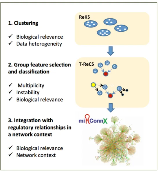
Figure 1.3 Overall approach of the proposed module-based biomarker discovery framework
1.6 CONTRIBUTIONS
Motivated by the abundance of recently available large-scale clinical data, and a need for a more biologically informed biomarker discovery method, an integrative, module-based framework for biomarker selection is developed and outlined in this dissertation. We highlight some of its key contributions.
ReKS
Computationally, this work contributes two novel algorithms to the community, both building on sound existing algorithms. The clustering algorithm, Recursive K-means Spectral Clustering (ReKS) (Figure 1.3 [1]), is one of the first to apply a recursive form of spectral clustering algorithm on high-dimensional clinical expression data. The second algorithm, Tree-guided Recursive Cluster Selection (T-ReCS) (Figure 1.3 [2]), offers a novel group variable selection framework based on local causal discovery theories. The two algorithms are integrated; the output of the clustering algorithm can be used to guide the feature selection process. Nevertheless, each can also be used separately as standalone algorithms. Aside from the application in high-throughput genomics data emphasized in this dissertation, both of these algorithms are general-purpose methods also applicable to other high-dimensional datasets with correlated variables.
To serve the biomedical community, we developed an interactive web-server, mirConnX
(Figure 1.3 [3]), to present an integrated transcriptional and post-transcriptional network. The mirConnX network is constructed from a comprehensive compilation of prior regulatory relationships and computational predictions, and integrated with user supplied condition-specific expression data. Since its introduction, mirConnX has assisted numerous1 users to explore their datasets in the context of regulatory relationships. An upcoming release of mirConnX 2.0 will further integrate with the aforementioned biomarker discovery framework. The selected discriminative gene and miRNA clusters are annotated with curated and putative regulatory relationships, and presented in a network context. We hope that through our proposed module-based biomarker discovery framework, integrated in the mirConnX environment, we will further
1As of September 2013, mirConnX has had 2407 unique visitors
assist the biomedical community in generating actionable biological hypothesis and advancing toward the ultimate goal of improving understanding of complex disease formation.
1.7 OVERVIEW AND ORGANIZATION
This dissertation is organized as follows.
In Chapter 2, ReKS, a recursive spectral clustering method developed to partition genes into a tree structure is described in detail. The algorithm is evaluated against other popular clustering methods on several metrics and on a benchmarking dataset. Its applications to large-scale clinical datasets are presented. We also described a formal prior information incorporation framework for incorporating prior knowledge such as protein-protein interaction, domain knowledge or pathway information. We additionally pointed to a potential future strategy for improving stability using a perturbation algorithm.
Chapter 3 presents the group variable selection algorithm, T-ReCS, which exploits the tree structure generated previously to guide its search for discriminative group variables. Relevant background concepts are introduced and the rationale for the method is explained in detail. The performance of the algorithm is evaluated on simulated, benchmarking and real data. In Chapter 4, we describe the details of the method for constructing the backend of the integrative web server mirConnX, and highlight several examples of its applications. We also provide a demonstration of the proposed integrative analysis on a set of melanoma gene and miRNA expression dataset to reveal the utility of our integrated framework, and illustrate our vision for the upcoming release of the web server.
2.0 REKS: RECURSIVE K-MEANS SPECTRAL CLUSTERING
Clustering of gene expression data simplifies subsequent data analyses and forms the basis of numerous approaches for biomarker identification, prediction of clinical outcome, and therapeutic strategies. The most popular clustering methods such as K-means and hierarchical clustering are intuitive and easy to use, but they require arbitrary choices on their various parameters (number of clusters for K-means, and a threshold to cut the tree for hierarchical clustering). Human disease gene expression data are in general more difficult to cluster efficiently due to background (genotype) heterogeneity, disease stage and progression differences and disease subtyping; all of which cause gene expression datasets to be more heterogeneous. Spectral clustering has been recently introduced in many fields as a promising alternative to standard clustering methods. The idea is that pairwise comparisons can help reveal global features through the eigen techniques. In this paper, we developed a new method (ReKS) for clustering disease gene expression data based on a recursive spectral clustering algorithm. We benchmarked ReKS on three large-scale cancer datasets and we compared it to different clustering methods with respect to execution time, background models and external biological knowledge. We found ReKS to be superior to the hierarchical methods and equally good to K -means, but much faster than them and without the requirement of a priori knowledge of K. Overall, we believe that recursive spectral clustering offers an attractive alternative for efficient clustering of human disease data.
2.1 CLUSTERING OVERVIEW AND MOTIVATING EXAMPLE
The explosion of gene expression and other data collection from thousands of patients of several diseases has created novel questions about their meaningful organization and analysis. The Cancer Genome Atlas (TCGA) [22] initiative for example provides large heterogeneous datasets from patients with different types of cancers including breast, ovarian and glioblastoma. However, unlike data from model organisms and cell lines that inherently contain uniform genetic background, and where experiments are conducted under controlled conditions, disease samples are typically much more heterogeneous. Differences in the genetic background of the subjects, disease stage, progression, and severity as well as the presence of disease subtypes contribute to the overall heterogeneity. Discovering genes or features that are most relevant to the disease in question and identifying disease subtypes from such heterogeneous data remains an open problem.
Clustering, the unsupervised grouping of data vectors into classes with similar properties is a powerful technique that can help solve this problem by reducing the number of features one has to analyze and by extracting important information directly from data when prior knowledge is not available. As such, it has formed the basis of many feature selection and classification methods [65], [66]. Hierarchical and data partitioning algorithms (like K-means) have been used widely in many domains [67] including biology [68], [69]. They have become very popular due to their intuitiveness, ease of use, and availability of software. Their biggest drawbacks come from the usually arbitrary selection of parameters, such as the optimal number of clusters (for K -means) or an appropriate threshold for cutting the tree (for hierarchical clustering).
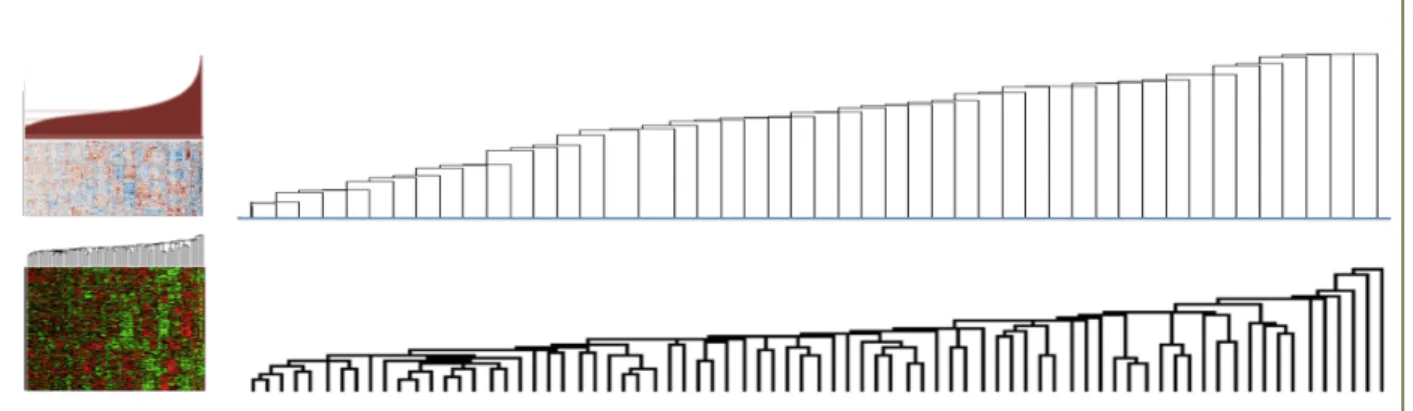
[69]. However, the heterogeneity of the disease samples hinders their efficiency in them. Figure 2.1 shows an example of such a dataset; a dendrogram produced from the breast cancer TCGA data, in comparison to dendrogram generated from the less heterogeneous yeast expression data. It is obvious that the structure of the data makes it difficult to find a threshold to prune the tree to produce a satisfactory number of clusters, since every newly formed cluster is joined with a singleton node each time. Thus, despite its popularity, classical hierarchical clustering frequently performs poorly in discovering a satisfactory group structure within gene expression data. Tight clustering [70] and fuzzy clustering [71] attempt to build more biologically informative clusters either by focusing only on closely related genes while ignoring the rest, or by allowing overlap in cluster memberships. However, both methods suffer from long execution times. Similarly, Affinity Propagation [72] has been applied on gene clustering successfully but a significant execution time trade-off exists.
More recently, spectral clustering approaches have been used for data classification, regression and dimensionality reduction in a wide variety of domains, and have also been applied to gene expression data [73]. The spectral clustering formulation requires building a network of genes, encoding their pairwise interactions as edge weights, and analyzing the eigenvectors and eigenvalues of a matrix derived from such a network. To our knowledge, no systematic attempt has been made to-date to test and compare the performance of existing clustering methods in large-scale disease gene expression data, perhaps due to unavailability of suitable size datasets. In this paper, we evaluate the standard K-means and hierarchical clustering methods on three large TCGA datasets. The evaluation is performed using intrinsic measures and external information. We introduce ReKS (Recursive K-means Spectral clustering), and compare it to the two aforementioned methods on the TCGA data. ReKS leverages the global similarity structure
that spectral clustering provides, while saving on computing time by performing recursion. At each recursion step, we exploit the distribution of eigenvalues to select the optimal number of partitions, thus eliminating the need for pre-specifying K. We show that ReKS is very useful in deriving important biological information from patient gene expression data. Furthermore, we show how to add prior information from KEGG [74] pathway to refine the cluster boundaries.
Figure 2.1 Clustering patient data is more difficult than cell-based data.
Partial views of dendrograms constructed from hierarchical clustering of the TCGA Breast Cancer expression data (top) and the yeast expression data (from Spellman et al. [75]). The dendrograms suggest that it is easier to select a threshold to prune the tree and generate potentially meaningful clusters for the yeast data but not so for the breast cancer data.
2.2 SPECTRAL CLUSTERING
The spectral clustering formulation requires building a network of genes, encoding their pairwise interactions as edge weights, and analyzing the vectors and eigenvalues of a matrix derived from such a network. This procedure is well established in the literature [76] so here we limit our discussion to the main points of the algorithm and use a Markov chain perspective to help us reason further about the idiosyncrasies of the algorithm when applied to cancer expression data.
A convenient framework for understanding the spectral method is to consider the partitioning of an undirected graph 𝐺 =< 𝑉,𝐸 > into a set of distinct clusters. Here the genes are represented as vertices 𝑣! for 𝑖=1…𝑁 where 𝑁 is the total number of genes and network edges have weights 𝑤!" that are non-negative symmetric (𝑤!" =𝑤!") to encode the strength of interaction between a given pair of genes. Affinities denote how likely it is for a pair of genes to belong to the same group. Here we used as affinities a modified form of the correlation coefficient 𝜌!", calculated on the gene expression vectors:
𝑤!" = 𝑒𝑥𝑝 − 𝑠𝑖𝑛!"##$%(!!") !
!
(2.1)
This is distance measure previously found to give empirical success in the clustering of gene expression data [73]. Note that high affinities correspond to pairs of genes that are likely to belong in the same group (e.g., participate in a pathway). In this paper, we ensured that the network is connected so that there is a path between any two nodes of the network. Our goal is to group genes into distinct clusters so that genes within each group are highly connected to each other, while genes in distinct clusters are dissimilar.
Spectral methods use local (pairwise) similarity (affinity) measurements between the nodes to reveal global properties of the dataset. The global properties that emerge are best understood in terms of a random walk formulation on the network [77]–[79]. The random walk is initiated by constructing a Markov transition matrix over the edge weights. Representing the matrix of affinities 𝑤!" by 𝑊 and defining the degree of a node by 𝑑! = !𝑤!", a Markov transition matrix 𝑀 can be defined over the edge weights by
where 𝐷 is a diagonal matrix stacked with degree values 𝑑!. The transition matrix 𝑀 can be used to set up a diffusion process over the network. In particular, a starting distribution 𝑝! of the
Markov chain evolves to 𝑝= 𝑀!𝑝! after 𝛽 iterations. As 𝛽 approaches infinity, the Markov
chain can be shown to approach a stationary distribution:𝑀!= 𝜋1! is an outer product of 1 (a
column vector of 𝑁 1s) and 𝜋 (column vector of length 𝑁). It is easy to show that 𝜋 is uniquely given by: 𝜋! = 𝑑!/ !𝑑! and is the leading eigenvector of 𝑀:𝑀𝜋 =𝜋 with eigenvalue 1.
We can analyze the diffusion process analytically by using the eigenvectors and eigenvalues of M. From an eigen perspective the diffusion process can be seen as [78]:
𝑝! =𝜋+ 𝜆
!!𝐷!.!𝑢!𝑢!!𝐷!!.!𝑝! !
! (2.3)
where the eigenvalue 𝜆! = 1 is associated with stationary distribution 𝜋. The eigenvectors are arranged in decreasing order of their eigenvalues, so the second eigenvector 𝑢! perturbs the stationary distribution the most as 𝜆! ≥𝜆! for 𝑘> 2. The matrix 𝑢!𝑢!! has
elements 𝑢!,!×𝑢!,!, which means the genes that share the same sign in 𝑢! will have their transition probability increased, while transitions across points with different signs are decreased. A straightforward strategy for partitioning the network is to use the sign of the elements in 𝑢! to cluster the genes into two distinct groups.
Ng et al. [80] showed how this property translates to a condition of piecewise constancy on the form of leading eigenvectors, i.e. elements of the eigenvector have approximately the same value with-in each putative cluster. Specifically, it was shown that for 𝐾 weakly coupled clusters, the leading 𝐾 eigenvectors of the transition matrix 𝑀 will be roughly piecewise constant. The K-means spectral clustering method is a particular manner of employing the standard K-means algorithm on the elements of the leading 𝐾 eigenvectors to extract 𝐾 clusters
simultaneously. We follow the recipe in Ng et al. where instead of using a potentially non-symmetric matrix 𝑀, a symmetric normalized graph Laplacian 𝐿= 𝐷!!.!𝑊𝐷!!.!, whose
eigenvalues and eigenvectors are similarly related to 𝑀, is used for partitioning the graph. Spectral approaches have also some drawbacks. Their basic assumption of piecewise constancy in the form of leading eigenvectors need not hold on real data. Much work has been done to make this step robust, including the introduction of optimal cut ratios [81] and relaxations [82], [83] and highlighting the conditions under which these methods can be expected to perform well [78]. Spectral methods can be slow as they involve eigen decomposition of potentially large matrices (𝑂(𝑛!)). Recent attempts at addressing this issue include implementing the algorithm in parallel [84], speeding eigen decomposition with Nystrom approximations [85], building hierarchical transition matrices [86] and embedding distortion measures for faster analysis of large-scale datasets [87].
2.3 METHOD OVERVIEW
In this paper, we will pursue a recursive form of K-means spectral clustering (ReKS), apply it on cancer expression data from patients and understand the intrinsic structure of the data by establishing a baseline clustering result. ReKS first defines an affinity matrix of all pairwise similarities between genes. We reduce the computational burden with sparse matrices, such that each gene is connected to a small number of its neighbors (default: 15) with varying affinities, and extract only a small subspace of eigenpairs (default: 20). In each recursion step, we determine the most appropriate subspace in which to run K-means using the eigengap heuristic, which is to compute the ratio of successive eigenvalues and pick K of 𝑎𝑟𝑔𝑚𝑎𝑥!λ! λ!!!, for 𝑖 =
1 to 20. We apply the eigengap heuristic at each recursion level to determine the optimal number of partitions at that level. In addition, to improve the convergence of the K-means algorithm we initiate the algorithm with orthogonal seed points. For each newly formed cluster, we extract the corresponding affinity sub-matrix and repeat the procedure.
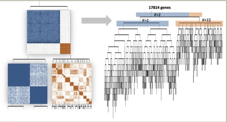
Figure 2.2 Demonstration of the ReKS method on the GBM dataset.
(Left) The first two iterations of K-means spectral decomposition recursions: two clusters are visible in the affinity map constructed from the entire dataset at the first level. From each, a new affinity matrix is constructed and spectral clustering repeated on the sub-affinity matrix. (Right) Complete tree obtained by ReKS iterations. Each leaf node corresponds to a gene cluster in the final partition.
In Figure 2.2(Left) we illustrate the top two levels of ReKS recursion on the GBM dataset. At level-1 an obvious partition exists for the original affinity matrix. The genes are split into two clusters at this node, and for each cluster, a new affinity matrix is computed. ReKS performs this procedure iteratively stopping when further split would cause all clusters to be 35 or smaller in size. The stopping threshold corresponds to the average number of genes that participate in a KEGG pathway. In the end, we arrive at a tree where each leaf node represents a
gene cluster. Note that with this procedure clusters of smaller than 35 genes could be obtained, for example due to an early split off the tree, as long as there is a cluster that is large in size. Figure 2.2(Right) presents the full tree generated by ReKS on the GBM dataset.
The complexity of ReKS is roughly 𝑂(𝑁!), N being the total number of genes to cluster. At every node of the tree, an SVD is performed at 𝑂(𝑑𝑛!), n being the number of genes at the node, and k-means is performed at 𝑂(𝑖,𝑘,𝑛,𝑑), where i is the number of iterations, d is the reduced dimension capped at 20, and k is the corresponding number of clusters <= 20. Since i is bounded and d and k are fixed to 20 and less, the k-means step is essentially linear to n. Assuming a balanced tree with each node having k=20 children, the overall complexity is
𝑘!𝑂(𝑑 !
!!
! )≈ !
!!! 𝑂(𝑁!), and 𝑂(𝑁!) in the worst case scenario with an extremely
unbalanced tree.
2.4 PERFORMANCE EVALUATION
2.4.1 Comparison to other methods on TCGA cancer data
2.4.1.1Data description
We applied ReKS on the three most complete TCGA gene expression datasets to date: Glioblastoma multiform (GBM) with a total of 575 tumor samples, Ovarian serous cystadenocarcinoma (OV) with a total of 590 tumor samples, and Breast invasive carcinoma (BRCA) with a total of 799 tumor samples. The level 3, normalized and gene-collapsed data obtained from the TCGA portal were downloaded and no further normalization was performed.
We compare our method against four other partition solutions: (1) average linkage hierarchical clustering, (2) average linkage hierarchical clustering on the spectral space, (3) K-‐means and (4) K-‐means on the spectral space. These algorithms are chosen to cover a range of common clustering techniques and clustering assumptions.
2.4.1.2Comparison of ReKS and other clustering strategies on TCGA data
Agglomerative clustering methods build a hierarchy of clusters from bottom up. It is perhaps the most popular on gene expression data analysis [88], due to its ease of use and readily available implementations. We performed hierarchical agglomerative clustering using Euclidean distance and average linkage. A maximum number of clusters is specified to be comparable to the number of clusters K obtained when running ReKS. Since this choice might be considered favorable to ReKS, we also performed hierarchical clustering on the top three eigenvectors in the spectrum, using cosine distances to measure the distance on the resulted unit sphere. Note that hierarchical clustering is done from bottom up, using local similarities, and does not embed the global structure in its tree.
Similarly, standard K-‐means and K-‐means performed on the spectral space are included for benchmarking purposes. Given a number of clusters, K, the algorithm iteratively assigns members to centroids and re-‐adjusts the centroids of the clusters. K-‐ means tends to perform well as it directly optimizes the intra-‐cluster distances, but tends to be slow especially as K increases. Here we used the default implementation of the K-‐ means clustering algorithm in Matlab, with Euclidean distance, again using the K obtained from ReKS. We also ran K-‐means on the spectral space, effectively performing ReKS only
once without choosing an optimal number of eigenvectors to use, but instead using K top eigenvectors.
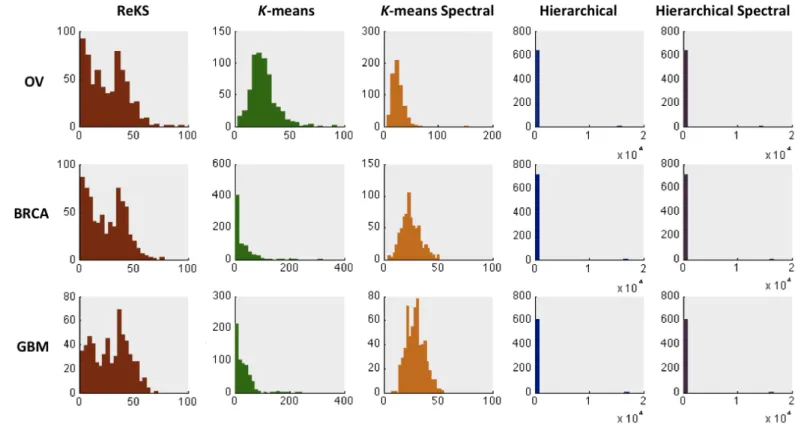
Shown in Figure 2.3 are the distributions of the cluster sizes when applying the five methods to the three TCGA datasets. Hierarchical clustering, whether in the original or the eigenspace, produces a very skewed distribution of cluster sizes that is possibly an artifact of focusing on only local similarities. The K-‐means methods and ReKS produce cluster sizes that span roughly the same range. However, the K-‐means methods produce distributions that are artificially Gaussian, with relatively little clusters that contain small number of genes.
2.4.1.3Cluster quality evaluation
We evaluate the quality of the clusters obtained from each of the five methods (ReKS, K-means,
K-means spectral, Hierarchical, Hierarchical spectral) using both intrinsic, statistical measures as well as external biological evidence, as detailed in the sections below.
• Calinski-Harabasz
To evaluate the quality of the clusters, we used the Calinski-H[arabasz measure [89], defined by:
𝐶𝐻= !"#$%&/(!"#$%&/(!!!)!!!) (2.4)
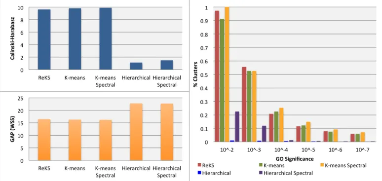
where 𝑡𝑟𝑎𝑐𝑒𝐵 denotes the error sum of squares between different clusters, 𝑡𝑟𝑎𝑐𝑒𝑀 is the intra-‐cluster square differences, 𝑚 is the number of objects assigned to the 𝑖!! cluster, and 𝐾 is number of clusters. This statistic is effectively an adjusted measure of the ratio of between-‐ vs. within-‐ group dispersion matrices. A larger value denotes a higher compactness of the cluster compared to the inter-‐cluster distances. Figure 2.4(Left) shows the performance of ReKS compared across other methods. Not surprisingly, ReKS outperforms hierarchical clustering in both the original data space as well as the spectral space, as hierarchical clustering produces some very large clusters with no apparent internal cohesion. The K-‐means based methods and ReKS are comparable in terms of cluster separation across the datasets.
• GAP Statistic
The Gap statistic was proposed as a way to determine optimal cluster size [90]. In short, it is the log ratio of a reference within-cluster sum of square errors over the observed within-cluster sum of squares errors. The reference is usually built from a permutated set of genes that form 𝐾 random clusters. Since we are comparing the (five) methods across the same dataset with the same 𝐾, it is fair to compare the performance of the observed within sum-of squares error only. With this direct proxy, ReKS performs at the same level as K-means based methods (shown in Figure 2.4(Left), and achieved a significantly lower sum-of-square distances than the hierarchical methods.
• Gene Ontology Enrichment
Since no ground truth exists for gene cluster partition, we examine the overall quality of the clusters in terms of the amount of enrichment for Gene Ontology (GO) annotations. For each
Figure 2.4 Performance of ReKS compared to other methods.
(Left) Cluster validity comparison with other methods using the Calinski-Harabasz and the GAP statistics (Right) Gene Ontology(GO) enrichment across different range of p-values
cluster, we test for GO enrichment using a variant of the Fisher’s exact test, as described in the
weight01 algorithm of the topGO [91] package in R. The significance level of the test indicates the degree a particular GO annotation is over-represented in a given cluster. For a partition, we calculate the proportion of clusters annotated with a GO term at a 𝑝-value threshold. If a cluster has less than five members, the test is not performed. As shown in Figure 2.4(Right), compared to hierarchical clustering, we observe that ReKS contains higher percentage of clusters that are significant at the specified levels, and especially so with more stringent p-value thresholds, and performs roughly the same as K-means methods. Finally, we observe that the spectral methods tend to perform better than their non-spectral counter-parts.
• Execution Time
Table 2.1 shows the execution time of the five methods on a 3.4 GHz Intel Core i7 CPU. ReKS is slower than hierarchical clustering but compares favorably to K-means methods.
Table 2.1 ReKS average execution time compared to other methods
Methods ReKS K-means K-means
Spectral Hierarchical Hierarchical Spectral
Execution time 373s 6000s 1774s 90s 22s
2.4.2 Benchmarking against patient data
Since gold standard for gene clustering does not exist, we resort to benchmarking ReKS on a set of well established microarray data where the goal is to cluster patients into known disease subtypes. de Souto et al. [88] compiled a list of 35 datasets from Affymetrix and cDNA microarrays . They performed a comprehensive analysis of seven different clustering methods and coupled them with seven definitions of proximity measure for clustering cancer tissues.

![Table 1.2 Tumor-associated microRNAs and their validated target genes [51]](https://thumb-us.123doks.com/thumbv2/123dok_us/10155948.2917381/22.918.144.783.246.458/table-tumor-associated-micrornas-validated-target-genes.webp)