on
Special Hardware
Tom´
aˇ
s Davidoviˇ
c
Thesis for obtaining the title of Doctor of Engineering Science (Dr.-Ing.) of the Faculty of Mathematics and Computer Science of Saarland University Saarbr¨ucken, Germany, May 2016
Saarland University, Saarbr¨ucken, Germany Committee chair:
Prof. Dr. Sebastian Hack
Saarland University, Saarbr¨ucken, Germany Reviewers:
Prof. Dr.-Ing. Philipp Slusallek
Saarland University, Intel VCI, and DFKI, Saarbr¨ucken, Germany Dr.-Ing. Habil. Karol Myszkowski
MPI Informatik, Saarbr¨ucken, Germany Doc. Ing. Jaroslav Kˇriv´anek, Ph.D.
Charles University, Faculty of Mathematics and Physics Praha, Czech Republic
Academic assistant: Dr. Andreas Nonnengart DFKI, Saarbr¨ucken, Germany Date of defense:
November 25th, 2016
Abstract
It cannot be denied that the developments in computer hardware and in computer algorithms strongly influence each other, with new instructions added to help with video processing, encryption, and in many other areas. At the same time, the current cap on single threaded performance and wide availability of multi-threaded processors has increased the focus on parallel algorithms. Both influences are extremely prominent in computer graphics, where the gaming and movie industries always strive for the best possible performance on the current, as well as future, hardware.
In this thesis we examine the hardware-algorithm synergies in the con-text of ray tracing and Monte-Carlo algorithms. First, we focus on the very basic element of all such algorithms – the casting of rays through a scene, and propose a dedicated hardware unit to accelerate this common operation. Then, we examine existing and novel implementations of many Monte-Carlo rendering algorithms on massively parallel hardware, as full hardware uti-lization is essential for peak performance. Lastly, we present an algorithm for tackling complex interreflections of glossy materials, which is designed to utilize both powerful processing units present in almost all current com-puters: the Central Processing Unit (CPU) and the Graphics Processing Unit (GPU). These three pieces combined show that it is always important to look at hardware-algorithm mapping on all levels of abstraction: instruc-tion, processor, and machine.
Kurzfassung
Zweifelsohne beeinflussen sich Computerhardware und Computeral-gorithmen gegenseitig in ihrer Entwicklung: Prozessoren bekommen neue Instruktionen, um zum Beispiel Videoverarbeitung, Verschl¨usselung oder an-dere Anwendungen zu beschleunigen. Gleichzeitig verst¨arkt sich der Fokus auf parallele Algorithmen, bedingt durch die limitierte Leistung von f¨ur einzelne Threads und die inzwischen breite Verfgbarkeit von multi-threaded Prozessoren. Beide Einfl¨usse sind im Grafikbereich besonders stark , wo es z.B. f¨ur die Spiele- und Filmindustrie wichtig ist, die bestm¨ogliche Leistung zu erreichen, sowohl auf derzeitiger und zuk¨unftiger Hardware
In Rahmen dieser Arbeit untersuchen wir die Synergie von Hardware und Algorithmen anhand von Ray-Tracing- und Monte-Carlo-Algorithmen. Zuerst betrachten wir einen grundlegenden Hardware-Bausteins f¨ur alle diese Algorithmen, die Strahlenverfolgung in einer Szene, und pr¨asentieren eine spezielle Hardware-Einheit zur deren Beschleunigung. Anschließend unter-suchen wir existierende und neue Implementierungen verschiedener Monte-Carlo-Algorithmen auf massiv-paralleler Hardware, wobei die maximale Auslastung der Hardware im Fokus steht. Abschließend stellen wir dann einen Algorithmus zur Berechnung von komplexen Beleuchtungseffekten bei gl¨anzenden Materialien vor, der versucht, die heute fast ¨uberall vorhandene Kombination aus Hauptprozessor (CPU) und Grafikprozessor (GPU) op-timal auszunutzen. Zusammen zeigen diese drei Aspekte der Arbeit, wie wichtig es ist, Hardware und Algorithmen auf allen Ebenen gleichzeitig zu betrachten: Auf den Ebenen einzelner Instruktionen, eines Prozessors bzw. eines gesamten Systems.
Acknowledgments
No long term project is possible without support and inspiration from many people from all walks of life.
First and foremost, I would like to thank my supervisor Philipp Slusallek for giving me the chance to switch fields from hardware to graphics, for his guidance in the research, and the enthusiasm with which he intro-duced me to many other greats of the graphics field. I would also like to thank the Saarland University and the Intel Visual Computing Institute for providing funding of my research.
Special thanks also go to my two main collaborators, Jaroslav Kˇriv´anek and Miloˇs Haˇsan, whose fresh perspective was always there when my inspiration was running dry. I would also like to thank my friends and colleagues at the Saarland University: Iliyan Georgiev, Stefan Popov, Javor Kalojanov, Luk´aˇs Marˇs´alek, Beata Turoˇnov´a, Martin ˇCad´ık, Vincent Pego-raro, and Ralf Karrenberg for ideas, support, distractions and generally the best atmosphere a man could want in a time.
Sebastian Sylwan and Luca Fascione are solely responsible for fulfilling an impossible childhood dream of mine by giving me the opportunity to do an internship at Weta Digital and, in turn, be an active participant on bringing the works of Tolkien to life. The thanks also belong to the anonymous reviewers, whose comments always helped to produce a better and clearer paper.
And last but not least, I would like to thank all my friends and family, who supported me throughout the years in all the major decisions I had to make.
1 Introduction 1
1.1 Our contributions. . . 4
2 Background 7 2.1 Light Transport. . . 8
2.1.1 Radiometric Quantities . . . 8
2.1.2 The Rendering Equation . . . 9
2.1.3 The Ray Tracing Operator . . . 10
2.1.4 The Path Integral Formulation . . . 11
2.1.5 The Bidirectional Scattering Distribution Function . . 12
2.2 Monte Carlo Integration . . . 14
2.2.1 Random Variables . . . 14
2.2.2 Monte Carlo Estimator and Its Error. . . 15
2.2.3 Efficient Sampling of Monte Carlo Estimator . . . 16
2.3 Rendering Techniques . . . 18
2.3.1 Direct Illumination . . . 18
2.3.2 Whitted-style Ray Tracing . . . 20
2.3.3 Path Tracing . . . 21
2.3.4 Bidirectional Path Tracing . . . 23
2.3.5 (Progressive) Photon Mapping . . . 24
2.3.6 Virtual Point Lights . . . 27
2.4 Acceleration Structures . . . 29
2.4.1 Ray Tracing Acceleration . . . 29
2.4.2 Photon Mapping Acceleration . . . 33
2.5 Hardware Acceleration . . . 36
2.5.1 Basics of Single Instruction Multiple Data . . . 36
2.5.2 General-Purpose computation on Graphics Processing Units . . . 38
2.5.3 Dedicated Ray Casting Units . . . 41
3 A Dedicated Ray Traversal Engine 47 3.1 Ray traversal engine . . . 49
3.1.1 Design blocks . . . 50
3.1.2 RTE synthesis . . . 51
3.2 Simulator architecture . . . 52
3.2.1 Shader models . . . 53
3.2.2 Acceleration structure partitioning . . . 53
3.3 Results. . . 54
3.3.1 Standard implementation . . . 54
3.3.2 Treelet implementation . . . 56
3.3.3 Using BVH . . . 58
3.4 Conclusion . . . 59
4 Light Transport Simulation on the GPU 63 4.1 Related Work . . . 64 4.2 Overview . . . 65 4.2.1 Terminology . . . 67 4.2.2 Testing Setup . . . 68 4.3 Path Tracing . . . 69 4.3.1 Algorithm Overview . . . 69
4.3.2 Survey of Existing GPU Implementations . . . 70
4.3.3 Proposed Alternative Implementations . . . 74
4.3.4 Results and Discussion . . . 76
4.3.5 Conclusion . . . 79
4.4 Bidirectional Path Tracing. . . 80
4.4.1 Algorithm Overview . . . 80
4.4.2 Survey of Existing GPU Implementations . . . 81
4.4.3 Proposed Alternative: Light Vertex Cache BPT. . . . 83
4.4.4 Results and discussion . . . 85
4.4.5 Conclusions . . . 87
4.5 Photon Mapping-Based Approaches . . . 88
4.5.1 Survey of Existing GPU Implementations of Photon Map Search Structures . . . 90
4.5.2 Rectified Stochastic Hash Grid . . . 92
4.5.3 Implementation Detail: Improved Hash Grid Query . 93 4.5.4 Results and Dicussion . . . 94
4.5.5 Conclusions . . . 97
4.6 Vertex Connection and Merging . . . 97
4.6.1 Algorithm Overview . . . 98
4.6.2 Proposed GPU Implementation . . . 98
4.6.3 Results and Discussion . . . 98
4.7 Algorithm Comparison . . . 99
4.7.1 Path Tracing . . . 101
4.7.2 Bidirectional Path Tracing . . . 101
4.7.3 Photon Mapping-based Methods . . . 102
4.7.4 Vertex Connection and Merging . . . 103
5 Global and Local VPLs 107
5.1 Related Work . . . 109
5.2 Overview . . . 111
5.3 Visibility Clustering for Global Lights . . . 114
5.4 Local Lights . . . 117
5.5 Implementation Details . . . 118
5.6 Results. . . 119
5.7 Conclusion . . . 125
6 Conclusion 129 A Supplemental Material for Light Transport Simulation on the GPU 135 A.1 Path Tracing . . . 135
A.2 Bidirectional Path Tracing. . . 135
A.3 Algorithm Comparison . . . 136
B Supplemental Material for Global and Local VPLs 147 B.1 Stochastic Progressive Photon Mapping . . . 147
2.1 Global Illumination examples . . . 7
2.2 Lambert’s Law . . . 9
2.3 Used BSDFs . . . 13
2.4 Pinhole Camera. . . 18
2.5 Direct Illumination . . . 19
2.6 Direct illumination limitations . . . 20
2.7 The Whitted-style ray tracing . . . 20
2.8 Naive Path Tracing. . . 22
2.9 Path Tracing with Next Event Estimation . . . 23
2.10 Bidirectional Path Tracing failure . . . 24
2.11 Bidirectional Path Tracing vs Photon Mapping . . . 25
2.12 Photon Mapping paths . . . 26
2.13 Virtual Point Lights . . . 27
2.14 2D Uniform Grid . . . 30
2.15 2D kd-tree . . . 31
2.16 2D Bounding Volume Hierarchy . . . 32
2.17 2D point kd-tree . . . 34
2.18 2D point Uniform Grid. . . 35
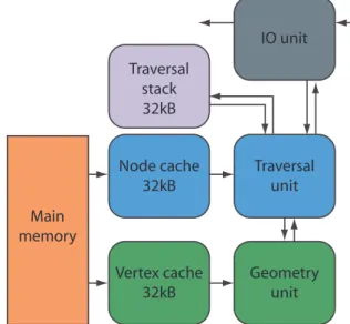
3.1 RTE block diagram. . . 50
4.1 Our test scenes. . . 68
4.2 Compaction . . . 72
4.3 Path Tracing Performance . . . 79
4.4 Bidirectional Path Tracing sample . . . 80
4.5 Reflected caustics . . . 86
4.6 Progressive Photon Mapping variants. . . 88
4.7 PPM, SPPM and PBPM on glossy surfaces . . . 90
4.8 Rectified Stochastic Hash Grid . . . 92
4.9 Vertex Connection and Merging . . . 98
4.10 Asymptotic convergence of all algorithms on all scenes . . . . 100
4.11 Convergence of PPM and BPT . . . 102
5.1 Comparison of our approach with Virtual Spherical Lights
(VSLs). . . 107
5.2 Conceptual overview of our algorithm . . . 115
5.3 Global light methods . . . 119
5.4 Local lights only . . . 121
5.5 Component separation . . . 122
5.6 Kitchen 1 . . . 123
5.7 Results. . . 124
A.1 Path tracing performance . . . 137
A.2 Complete performance results . . . 139
A.3 CoronaRoom results . . . 140
A.4 CoronaWatch results . . . 141
A.5 LivingRoom results . . . 142
A.6 BiolitFull results . . . 143
A.7 CrytekSponza results . . . 144
A.8 GrandCentral results . . . 145
B.1 Comparison with PPM and SPPM . . . 148
3.1 Results without treelets . . . 55
3.2 Results with treelets . . . 57
3.3 Acceleration structures . . . 59
4.1 Path Tracing Performance . . . 77
4.2 Summary of BPT memory requirements . . . 85
4.3 Relative BPT speed up . . . 87
4.4 WhileQuery speedup . . . 95
4.5 Acceleration Structure comparison . . . 95
4.6 PPM acceleration structure timings. . . 96
4.7 VCM performance . . . 99
5.1 Timing and statistics . . . 120
A.1 Relative BPT speed up . . . 138
NaivePTmk Naive Path Tracing (multiple kernels) . . . 70
RegenerationPTmk Path Tracing with Regeneration (multiple kernels) 71 StreamingPTmk Streaming Path Tracing with Regeneration . . . 73
NaivePTsk Naive Path Tracing (single kernel) . . . 75
RegenerationPTsk Path Tracing with Regeneration (single kernel) . 76 StreamingBPT Streaming Bidirectional Path Tracing with Re-generation . . . 82
LVC-BPT Light Vertex Cache BPT . . . 84
1 Building hash grid . . . 91
2 Hash Grid Query . . . 94
GLL Global and Local VPLs . . . 113
Introduction
In the past two decades, 3D computer graphics slowly became ubiquitous in our lives. It is an indisputable part of our entertainment as, in the almost twenty years since Toy Story was the first feature length 3D animated movie, 3D animation took over the field almost exclusively. The same is true for live action movies, where the posters moved from boasting that the movie does also contain computer-generated imagery to boasting that the movie does also contain practical effects. And, of course, computer games of just about any kind do not even need a mention.
But it is not just the obvious fields where 3D graphics plays an im-portant role. It is also used in architecture to visualize buildings and offices before they are built, in design to both pitch the initial designs and to re-duce the number of model iterations before the final product is approved, in bioinformatics where 3D visualization of proteins with shadows and other lighting effects helps the researchers to better understand the protein struc-tures and their possible effects, and we could go on and on.
Therefore, it is no surprise that there is an ever-present push for a higher realism of graphics, be it more detail, better materials, or more realistic illumination. In car design, faithful 3D visualization allows the car manufacturers to reduce the number of physical prototypes, as well as quickly showing the customers what a car would look like with a different paint or interior. In architecture, the game-like 3D graphics allows us to present the customers with a walk-through of a yet non-existent building. The more realistic illumination also allows evaluating how much light an office desk or a living room will get throughout the year. It could also, with sufficiently accurate models, prevent the effects of London’s “Walkie-Talkie” skyscraper, which focuses light on several London streets and melts plastic parts of cars parked there.
The importance of accurately representing the real world in visual ef-fects for action movies is indisputable, as the goal is to present the audience with imagery that is indistinguishable from reality, including – but not
ited to – creating whole environments and placing actors’ faces on stuntmen bodies. But the realism is also important in animated movies even though the audience knows from the start that the settings are not real. The artists rarely need completely photorealistic images but getting the indirect illu-mination, the color bleeding, the penumbra shadows, and other such effects right can still greatly enhance the image and leads to convincing realism. And these effects are, indeed, present in all the newer movies by all the big names in the industry such as Disney, DreamWorks, Pixar, and many others.
To achieve this ever-increasing demand for realism, the computer graphics has also evolved. At the very first, only the wireframe models, that is, the edges of the objects, were displayed. This approach gave the user a blueprint-like view of the scene and, for this very reason, it is still used in architecture and similar applications. However, despite the indis-putable advantages when it comes to design, the see-through nature is not really appealing for most applications.
The next step was to assign the objects with colors and then, for each pixel, display the color of the closest object seen through the pixel. It is also possible to assign each point of the object its own color to give a perception of surfacetexture such as wood or granite. This gives the users a basic idea about spatial relations of objects in the scene and in this simple form can be still seen today in basic kitchen planers and a similar software.
This approach has further evolved to allow more and more complex algorithms that determine the object’s color under a given pixel leading to today’s rasterization approach with fully programmable pixel shaders. These generally determine the color by evaluating camera position, light positions, and (multiple) textures. It is important to note that all of the computations are strictly local. That is, when computing a pixels color the program does not have any awareness about the rest of the scene and cannot, for example, determine whether it is in shadow in respect to particular light or not. While such limitations can, of course, be worked around, the workarounds always contain some kind of approximation that cannot achieve a completely faithful representation of the scene. For example, shadows can be approximated by storing, for each light and direction from it, the distance to the closest object in an approach called shadow mapping. As it obviously is not possible to store the distance for each direction, these directions are therefore discretized, leading to jagged shadow edge artifacts, with the artifact severity based on the resolution of the discretization.
To achieve the physical realism, we have to abandon these local illu-mination methods and, instead, focus onglobal illumination, inspired by the physics of light1. In the real world, photons are emitted from a light source 1For our purposes, we will consider only the ray optics approximation of the real light
and interact with the environment, reflected around until they are absorbed by a surface. If this surface is our camera’s sensor we register the photon and, after many such events, an image is formed. While we can simulate this exact behavior in a computer (the method is calledLight Tracing), the ratio of all surfaces in the scene that can absorb photons to the surface of the camera sensor is usually so large, that the method as described would be extremely inefficient. InPath Tracing we follow a reverse process, start-ing from the camera and interactstart-ing with surface until the path encounters a light source and the final contribution can be computed. Both of these methods, as well as many others that are based on the same principles, are collectively known as the light transport simulation, as they simulate how light is transported in a real world and along with physically plausible materials2 form the basis of the physically-based rendering.
In this thesis, we focus on accelerating these two basic approaches and the many algorithms that are based on them. First we look at the most common operation used: Finding the closest surface along a given ray. This is an essential building-block in all algorithms that mimic physics, as we simply need to know the next surface a photon will interact with. Is it also the single most important difference from the rasterization approaches, as it requires access to the whole scene. In Chapter3we look at the options of implementing this important operation in a dedicated hardware unit similar to rasterization units used on the modern GPUs.
To achieve a nice noise-free image with a digital camera, we want to capture, on average, somewhere between high tens and low hundreds of thousands of photons per pixel, depending on the sensitivity of the CCD sensor. While the paths used in computer graphics generally carry more in-formation than a single photon, e.g., each represents multiple wavelengths, we still often need tens to hundreds of paths per pixel, leading to tens to hundreds of millions of paths total, for a full HD image. Considering these paths are, at least in the basic approaches, completely independent and can all be computed in parallel, we can see why rendering is often called an embarrassingly parallel [Moler 1986] problem. A second important aspect to note about the paths simulated in a computer is that even paths that do not bring any contribution to the camera do come at cost. So, while in nature we can have many billions of photons emitted for each photon that is captured on the camera, our rendering algorithms have to be de-signed to maximize the number of paths that bring us relevant illumination information. In Chapter 4 we focus on these two objectives and explore mapping of progressively more and more advanced algorithms onto some of most powerful massively parallel hardware currently available.
2
Such materials are, for example, required to reflect at most as much energy as their receive in order to not violate the law of energy conservation. This somewhat obvious requirement was not common before physically-based rendering.
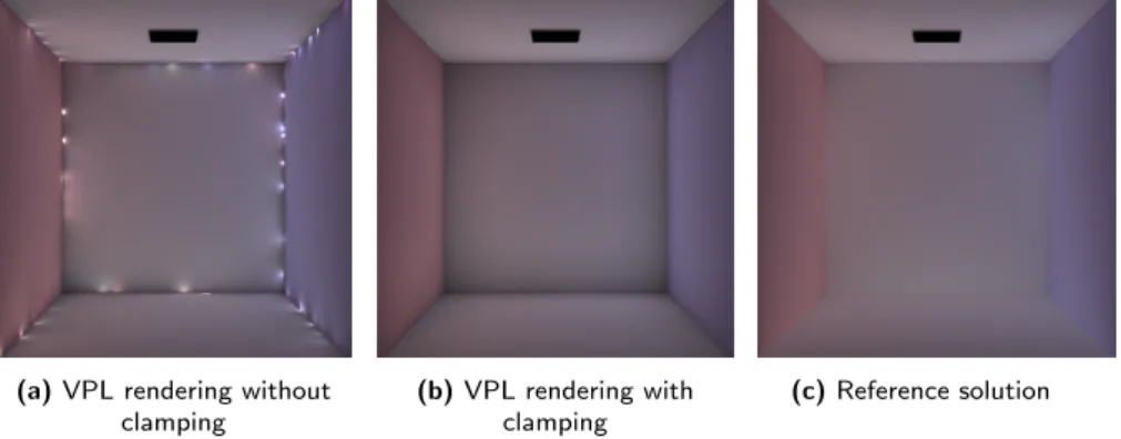
Unfortunately, even with the most advanced algorithms of today, there are still some scene configurations, such as stainless steel kitchens, that are extremely hard to sample efficiently, see Figure 5.6 for an example. On the other hand, many applications, such as fast design previews do not need exact physical accuracy but, instead, require a solution only accurate enough for the result to look convincing to the human eye. We explore this opportunity in Chapter 5, where we separate the problem into two parts, use different sets of approximation on each of these parts, and map the required steps to both CPU and GPU to utilize the full computing power of the modern computer.
1.1
Our contributions
The content of this thesis builds upon a number of previous work in the field, and its major contributions are based on previously published papers where the author was the main investigator. Below we present a summary of these contributions:
A Dedicated Ray Traversal Engine. (Section3) Finding the clos-est surface in a given direction is a fundamental operation in almost all photorealistic rendering algorithms. However, despite its ubiquitous nature and its significant cost that scales with the scene complexity, there still is little hardware acceleration available. Our first contri-bution is an evaluation of a dedicated Ray Traversal Engine hard-ware unit with a focus on its connection to a general purpose shading processor rather than just the ray traversal itself. We achieve this by modifying an existing Dynamic RPU design, synthesizing it with a state-of-the-art ASIC technology to obtain its characteristics and building a cycle accurate simulator of the unit. We show that such a unit could trace a significant number of rays for a fairly modest cost in both die area and bandwidth. These contributions are based on [Davidoviˇc et al. 2009] and [Davidoviˇc et al. 2011], where the author developed the VHDL code for hardware synthesis results, the SystemC simulation layer, performed majority of the tests, as well as wrote the main parts of the text.
Light Transport Simulation on the GPU.(Section4) When look-ing at a higher level of abstraction, the most important aspect in ren-dering is having as many efficient paths as possible. This is the goal of our next contribution where we focus on mapping algorithms onto a massively parallel, wide SIMD hardware, specifically the NVIDIA GPU cards using an already existing library for the ray tracing queries. We re-implement many previously proposed solutions for Path Trac-ing, Bidirectional Path TracTrac-ing, and Progressive Photon Mapping
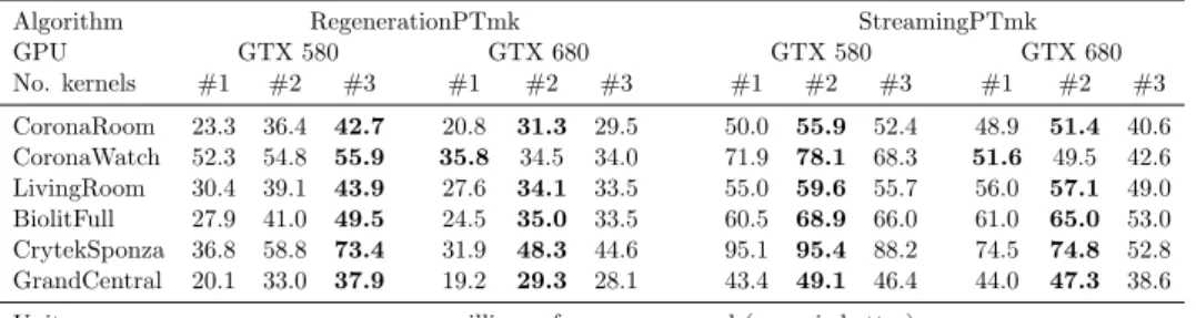
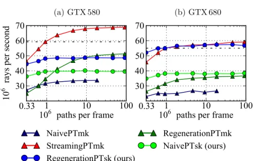
al-gorithms, augment the selection with some novel implementations of our own, and also provide the first GPU implementation of the Vertex Connection and Merging algorithm [Georgiev et al. 2012]. We test each of the algorithms on two generations of NVIDIA GPU and we present an extensive comparison of the various implementations, pro-viding detailed insight into their individual strengths and weaknesses with respect to the properties of the implementation platform. Fi-nally, to evaluate their relative performance in different scenarios we also provide a comparison of the algorithms across multiple scenes. This part of this thesis is based on [Davidoviˇc et al. 2014], where the author wrote the majority of the testing framework, proposed all the novel algorithms, performed the described experiments, and wrote majority of the technical sections.
Global and Local VPLs. (Section5) For our last major contribution presented in this thesis, we examine the extremely hard problem of in-terreflections in a highly glossy environment. In such an environment only a fairly narrow bands of paths have a significant contribution to the final image, and finding them by standard sampling techniques is difficult and time consuming. We propose to address this issue by separating the light transport into a global component, providing the overall illumination, and a local component, providing highly localized glossy reflections. This separation allows us to apply different approx-imations of each component which allows us to significantly increase the total number of contributing paths per pixel. The various steps of the algorithm are then split between the CPU and the GPU and executed in parallel to maximize the utilization of the used computer. This method was originally published in [Davidoviˇc et al. 2010], where the author wrote the majority of the code, proposed several key com-ponents on both local and global approximations, performed numerous experiments to evaluate feasibility of each element of the final algo-rithm, and wrote significant parts of the implementation details and results sections.
Other contributions. Our other contributions, not discussed in de-tail in this thesis, include investigation of similarities between ray trac-ing and rasterization [Davidoviˇc et al. 2012a], as well as further ad-vances in many-light methods on the GPU [Davidoviˇc et al. 2012b], and the first publicly available Vertex Connection and Merging imple-mentationSmallVCM [Davidoviˇc and Georgiev 2012]. The full list of publications is also a part of this thesis and can be found after the bibliography section (Section My Publications).
Background
(a)Direct illum. (b)Color bleeding (c)Ind. shadows (d)Full GI
Figure 2.1: Global Illumination examples. Direct illumination (2.1a) provides basic intuition about the scene but is far from realistic. Among the missing global illumination effects is color bleeding (2.1b), where light bounces off the red wall and colors the block in the middle. When the red wall receives a stronger illumination, it can also create indirect shadows (2.1c) behind the block. A combination of all the effects gives us full global illumination results (2.1d).
To render realistic global illumination effects, such as seen in Fig-ure 2.1, we first have to understand the basic physical principles of light propagation. In this chapter, we describe the basic concepts of light trans-port: The basic radiometric quantities used in light transport, the render-ing equation that describes light arrivrender-ing at each point in the scene, the ray tracing operator used to find the closest surface in a given direction, the Bidirectional Scattering Distribution Function (BSDF) used to describe material properties, and the path integral formulation of light transport. We refer to these terms in all the remaining chapters but significantly in Chap-ter 5, where we separate the rendering equation into two parts and solve them independently, each using a different set of approximations allowed by the separation.
Next, we introduce Monte Carlo integration as a general technique to solve the rendering equation, and describe several rendering techniques used to implement the Monte Carlo approach, such as Path Tracing, Bidirectional Path Tracing, and Virtual Point Lights. Chapter4 focuses on
tion of these methods on massively parallel machines. Thus, it describes the implementation details many of these methods in much greater detail.
We also give a basic overview of various acceleration structures both for ray tracing and for range queries used in Photon Mapping and its vari-ants. While not the main focus of this thesis, all our work uses these struc-tures in many variants and we refer to them throughout the remaining chap-ters.
In the last section we focus on hardware acceleration available for ren-dering. Namely we introduce the concept of Single Instruction Multiple Data (SIMD), used on the CPU, the GPU, as well as many dedicated ray trac-ing hardware solutions. Then, we introduce the principles and challenges of General-Purpose computing on Graphics Processing Units (GPGPU), which plays a major roles in Chapters4and5where we focus on various solutions to rendering equation on GPUs. Lastly, we introduce the concept of ded-icated hardware ray casting units as an alternative to standard hardware rasterization units and describe the issues encountered when designing such a unit. This is used as a basis for Chapter 3 where we describe integration of one such unit in a larger system.
2.1
Light Transport
In the following section we give a brief overview of light transport theory that describes distribution and interaction of the light with a scene. To reduce the complexity of the problem we use several common simplifications of light transport. Namely we do not consider light polarization, material fluorescence (re-emitting light at a different wavelength), and we assume that basic medium in which light propagates is vacuum, not air. We refer the readers to [Pharr and Humphreys 2004], [Dutr´e et al. 2006], [Veach 1997], and [Georgiev 2015] for more detailed discussion.
2.1.1 Radiometric Quantities
The basic quantity used in light transport isRadiant flux (orpower), which represents the total amount of energy passing through a region of space per unit time. It is denoted by Φ, measured in Watts.
The area density of flux arriving at a surface is calledirradiance (E), the area density of flux leaving a surface is called radiosity (B), both area measured in W/m2.
E = Φi
A B =
Φo
A (2.1)
Lambert’s Law states that the amount of light arriving at a sur-face is proportional to the cosine of the angle θ between the surface normal and the light direction. Figure 2.2 shows two examples us-ing orthogonally emittus-ing light sources A. In the first case (left),
A A
B ɵ C
Figure 2.2: Lambert’s Law. For an area light with the same areaA, the illuminated area and, in turn, irra-diance depend on the cosine of the angleθ.
the arriving light is perpendicular to the surface, the light source areaAis equal to the receiving areaB, and therefore:
EB =
Φ
B =
Φ
A =BA (2.2)
In the second case (right), the light arrives at an angle such that the receiving areaC
is larger. Then the following relation holds EC =
Φ
C =
Φ cosθ
A =BAcosθ (2.3)
A more general variant of Equation 2.1, that accounts for non-constant flux arriv-ing at the pointx, is given as:
E(x) = dΦ
dA (2.4)
The most important radiometric quantity isRadiance(L). It is defined as flux per unit area (perpendicular to the direction of the flux), per unit solid angle: L(x, ω) = d 2Φ dωdA⊥ = d2Φ dωdAcosθ (2.5) where dA⊥ is the projected area of dA onto the direction dω, andθ is the angle between ω and the surface normal. Intuitively, it can be seen as the amount of light coming from an infinitely small set of directions centered aroundω and arriving at an infinitely small area around a pointx. As such, it is the answer to the question “How much light arrives at this point from that direction?”.
An important property used in virtually all rendering algorithms is that radiance changes only when there is an interaction with either a surface or with a participating media (e.g., fog or smoke). For a pointx in empty space we therefore write:
Lo(x, ω) =Li(x,−ω) (2.6)
where Lo(x, ω) is radiance leaving the point x in the direction ω and
Li(x,−ω) is radiance arriving at the point xfrom the direction−ω.
2.1.2 The Rendering Equation
The light distribution in a scene is most often modeled using therendering equation by Kajiya [1986]:
Lo(x, ωo) =Le(x, ωo) +
Z
Ω+
It says that the radiance leaving a point x in a direction ωo, Lo(x, ωo), is
equal to the radiance emitted from that point in that direction Le(x, ωo)
plus the incoming radianceLi(x, ωi) from the whole upper hemisphere Ω+,
multiplied by the Bidirectional Reflectance Distribution Function (BRDF) fr(x, ωo, ωi) (see Section 2.1.5 for details) and the cosine of the angle θi
between incoming light direction and surface normal.
In this formulation the equation can describe only light reflection, omitting such important phenomena as refraction on glass. The equation can be extended to integration over the whole sphere Ω around point x [Veach 1997]. The function f(.) then becomesBidirectional Scattering Distribution Function (BSDF).
The rendering equation, as introduced above, assumes light of a sin-gle wavelength. Therefore, both L and f(.) are also parametrized by the wavelength λ. Most commonly, rendering systems use only three pseudo-wavelengths: red, green, and blue; which directly map to RGB used in common cameras and displays. However, to achieve effects like dispersion (e.g., rainbow), more wavelengths are needed.
2.1.3 The Ray Tracing Operator
The rendering equation (Equation 2.7) presents light interactions locally with respect to the point x. However, to solve for illumination globally we have to obtain the incoming radianceLi(x, ωi) from the hemisphere.
For the sake of simplicity, let us assume that light interactions can happen only on surfaces, i.e., the scene contains no participating media such as smoke, fog, or, indeed, air. From Equation2.6it follows that theLi(x, ωi)
will be equal to the reflectanceLo(x0,−ωi) at a pointx0, found along the ray
starting at the pointxin the directionωi. This pointx0 will lie on a surface
and, as we do not allow light to pass through surfaces without interaction, it will also lie on the closest such surface.
The ray tracing operator h(x, ω) provides us with an efficient way to denote such points and lets us rewrite the rendering equation in the following, recursive, way:
Lo(x, ωo) =Le(x, ωo) +
Z
Ω+
fr(x, ωo, ωi)Lo(h(x, ωi),−ωi) cosθidωi (2.8)
that is, the outgoing radiance at the point x is equal to the emitted radi-ance at that point, plus illumination from surfaces visible from the pointx, integrated over directionsωi.
This leads us to the notion that the illumination could be integrated not only over the hemisphere over the pointx, but, instead, over all surfaces visible from the point x. The resulting surface area formulation of the
rendering equation reads as follows: Lo(x, ωo) =Le(x, ωo) +
Z
A
fr(x, ωo,Ψ)Lo(y,−Ψ)V(x, y)G(x, y)dy (2.9)
where A are all surfaces of the scene, Ψ is the direction from point x to point y, V(x, y) is a visibility function, and G(x, y) is a geometric term. Visibility function is a simple binary function that has value of 1 when the path between x and y is not blocked by any objects and 0 otherwise. The geometric term comes from the conversion of differential area to differential solid angle and is given as:
G(x, y) = cos (Nx,Ψ) cos (Ny,−Ψ)
(x−y)2 (2.10)
whereNx andNy are normals at the points x and y, respectively.
This second formulation is very useful in the case where we know which surfaces are light sources and want to directly integrate the illumination from these light sources onto a given point.
2.1.4 The Path Integral Formulation
While the surface area measure formulation of the rendering equation (Equa-tion2.9) provides a well-defined formulation of the global illumination prob-lem, its recursive structure poses some limitations on understanding the problem. For example, in Chapter5 we will be separately solving the direct and indirect illumination, using Virtual Point Lights (see Section 2.3.6) to solve for the indirect illumination. The local understanding of the problem provided by the rendering equation would not be sufficient for that.
The path integral formulation introduced by Veach [Veach 1997], in-stead, poses the problem as a pure integration problem. In this formulation, the illumination on a pixel j can be computed as an integral over all light paths in the scene passing through the pixel:
Ij =
Z
Ω
fj(¯x)dµ(¯x), (2.11)
for all light paths ¯x. A path ¯x of a length k is defined as a (k+1)-tuple of vertices:
¯
x=x0x1. . . xk,
where each vertex lies on a surface. The length of the pathkis given by the number of path segments, each connecting two consecutive vertices, and the path therefore has k+ 1 vertices, where the vertex x0 is on a camera, and
the vertexxk is on a light source. Please note that this framework considers
only the last vertex of the path to be emissive and if a vertex can both emit and reflect light, these effects happen on different paths. However, this
is used only for theoretical analysis of the paths and poses no restrictions on the actual implementation, where traced path would generally represent multiple theoretical paths.
The space of all paths length kis Ωk and has a differential measure:
dµ(¯x) = dA(x0)dA(x1). . .dA(xk).
The final result of the integral is obtained when integrating over the space of all paths of all lengths Ω =S
k≥1Ωk, but it can also be separated and have
different path lengths solved through different means. For example, we can explicitly sample direct illumination (k≤ 2) and approximate the indirect illumination (k >2).
The path contribution function fj(¯x) is a product of the BRDF, the
visibility, and the geometry terms on the vertices of the path, finally multi-plied by the light emission:
fj(¯x) = k−1 Y i=1 fr(xi−1←xi←xi+1)V(xi↔xi+1)G(xi↔xi+1) ! | {z } path troughput Le(xk→xk−1), (2.12) where thefr(xi−1←xi←xi+1) is a formulation of BRDF that uses the
previ-ous and the next point along the pathxi−1,xi+1, to define the incoming and
outgoing directions (ωi, ωo) used in Equation2.13. The visibility function
V(xi↔xi+1) and the geometric term G(xi↔xi+1) are the same as in
Equa-tion 2.9, and the emission term Le(xk→xk−1) is, again, using a previous
point on a path to define the outgoing direction. The product of the BRDF, visibility, and geometric terms is also sometimes calledpath throughput, and represents a fraction of the radiance that is transported from the light source along this path.
The single most useful feature of this formulation is that we can gen-erate the path using any sampling technique as long as we can define a probability of each of the path vertices. That is, unlike the Equations 2.7 and 2.9, we are not bound by following the path from the camera into the scene.
2.1.5 The Bidirectional Scattering Distribution Function
The last element of the rendering equation that needs to be discussed is theBidirectional Scattering Distribution Function, which defines the visual appearance of objects in the scene. It gives an answer to the question: “If we shine light at the surface from direction ωi, how much light is reflected
towards the observer in directionωo”. Formally we write:
f(x, ωo, ωi) =
dLo(x, ωo)
Li(x, ωi) cosθidωi
(a)Diffuse (b)Phong (c)Ward (d)Mirror (e)Glass
Figure 2.3: Five BSDFs used in all the scenes throughout this work.
When bothωiandωoare in the same hemisphere (with respect to the surface
normal) we are talking about bidirectional reflectance distribution function (BRDF). When they are in the opposite hemispheres, we are talking about bidirectional transmittance distribution function (BTDF).
The total energy of reflected and transmitted light cannot exceed the total energy of incident light. All physically based BSDFs therefore have to obey the following energy conservation condition:
∀ωo,
Z
Ω
f(x, ωo, ωi) cosθidωi≤1. (2.14)
This integral representsalbedo, the total amount of energy that the material can reflect. In practice no materials have albedo equal to 1.
The second important condition for physically-based BRDFs (not BTDFs) is their symmetry (follows from Helmholtz reciprocity principle [Helmholtz 1867, Hapke 2012]). It states that for all pairs of ωo and ωi,
fr(x, ωi, ωo) =fr(x, ωo, ωi). That is, the surface will reflect the light in the
same way when we exchange the light source and the observer.
Figure 2.3presents five common BSDFs. Diffuse BRDF (2.3a) repre-sents rough surfaces like matted white paint, whileglossy BRDF (2.3band 2.3c) are used to represent surfaces with smooth finish. There are many dif-ferent glossy BRDF models ranging from purely empirical models, such as Phong BRDF [Phong 1975], to models that are derived from the surface mi-crostructures (Cook BRDF [Cook and Torrance 1981], Ward BRDF [Ward 1992]), and models that are used to represent measurements of actual ma-terials (Lafortune BRDF [Lafortune et al. 1997]).
The last two BSDFs on the Figure 2.3 represent the idealized ver-sions ofperfectly specular materials, where light can contribute toLo(x, ωo)
from only a limited set of discrete directions ωi. Mirror BRDF (2.3d) is a
mathematically perfect mirror and the BRDF is non-zero only when ωi is
the perfect reflection of ωo. Glass BSDF (2.3e) follows a similar principle
with the refraction direction given bySnell’s Law and the ratio between the reflected and refracted energy given by Fresnel Equations. While this be-havior is not physically realizable, these idealized models are widely used as many rendering algorithms can utilize these simplifications for substantial
performance gains. We refer the readers to [Jenkins and White 1976] for detailed explanation of the underlying physics principles.
In our scenes we use all four introduced types of BSDFs. For glossy we mainly use the common Phong BRDF, as it is the BRDF of choice for many modeling programs from which we obtained our scenes. However for metal surfaces we switch to the Ward BRDF, as it offers a more faithful rep-resentation of metals, including support for anisotropy needed to represent, e.g., brushed aluminum.
2.2
Monte Carlo Integration
Neither the recursive integral equation, nor the path integral introduced in the previous section can be solved analytically, except in the most trivial cases. Solving these equations therefore relies on using numerical methods, most commonly Monte Carlo integration. In this section we give a brief overview of random variables, Monte Carlo integration, and its improve-ments using importance sampling. For more complete introduction into the problematic with respect to graphics we refer to [Pharr and Humphreys 2004,Georgiev 2015].
2.2.1 Random Variables
A random variable X is a variable whose value is subject to chance. The values come from some domain, which can be either discrete, e.g., a dice, or continuous, e.g., the probability that a bus arrives at a given time.
In the case of a dice, we have a random variable X that can have values from the discrete domain 1, 2, 3, 4, 5, 6. Assuming the dice is a fair dice, each of these values has the same probability pi = 16. The probability
of all values always has to sum up to 1 and, consequently, the maximum probability a single value can have is 1. Such value would be chosen in all cases and the variable would, de facto, cease to be random.
Further, we define acumulative distribution function (CDF) as: P(x) =P r[X≤x]. (2.15) It represents the probability of the random variableX achieving value of x or less. In the case of a dice we get: 16, 13, 12, 23, 56, 1. CDFs are often used to map a uniform random number ξ ∈[0,1) (a common output of random generators) to the random variableX.
In the case of continuous random variables, the number of possible values is infinite and the concept of each value having its assigned probability is not applicable. Instead, we introduce the concept of aprobability density function(PDF), which indicates the density of probability in an area around a given value. For example, a uniform random variable in the range [a, b] the value of the PDF is constant and equal to b−1a.
The PDFs are always positive and always integrate to one. The prob-ability that a valuex lies in an interval [a, b] is given as:
P(x∈[a, b]) =
Z b
a
p(x)dx (2.16) and he value of the CDF(x) is given as:
CDF(x) =P(t∈[−∞, x]) =
Z x
−∞
p(t)dt (2.17) The expected value E[X] of a random variable X is, intuitively, the mean value of theX. In the case of a dice, theE[X] = 16(1+2+3+4+5+6) = 3.5. Formally, the expected value is defined as:
E[X] = X i xipi (2.18) E[f(x)] = Z D f(x)p(x)dx (2.19) for the discrete (top) and the continuous (bottom) case, respectively.
Complementary to E[f(x)] is thevariance V[f(x)], representing how spread out the values off(x) are from their mean. It is defined as follows:
V[f(x)] = E
h
(f(x))2
i
−E[f(x)]2 (2.20) Variance is commonly used as a measure of quality of results of Monte Carlo integrator and the goal of many algorithmic improvements is to lower the variance while keeping the costs the same.
2.2.2 Monte Carlo Estimator and Its Error
Informally, the basic Monte Carlo integration works as follows: Given a function f(x) over a domain D, we randomly choose N samples from the domain, evaluate the functionf(x) at these samples and average the results.
More formally, for a one-dimensional integral F = Rb
af(x)dx and N
random samplesXi ∈[a, b], the Monte Carlo estimator is:
ˆ FN = 1 N N X i=1 f(Xi) p(Xi) . (2.21)
Its expected valueE[ ˆFN] is then equal to the integralF =
Rb
af(x)dx, when
the PDF p(Xi)>0 for all Xi, where the f(Xi)6= 0.
However, unless the N = ∞, the actual value of ˆFN can differ from
The mean square error (MSE) of an estimator measures its average squared error: MSE( ˆFN) = E[( ˆFN −F)2] = E[ ˆFN2]−2E[ ˆFN]F +F2 = (E[ ˆFN2]−E[ ˆFN]2) + (E[ ˆFN]2−2E[ ˆFN]F+F2) = V[ ˆFN] + (E[ ˆFN]−F)2, (2.22)
where (E[ ˆFN]−F) isbiasand represents the difference between the expected
value of the estimator ˆFN and the true value of the integralF. Given that
our estimator hasE[ ˆFN] =F, we can say that the mean square error of the
estimator is equal to its variance.
Theroot mean square error (RMSE) of an estimate is the square root of MSE: RMSE( ˆFN) = q MSE( ˆFN) = q V[ ˆFN] +Bias( ˆFN)2, (2.23)
is expressed in the same units as the estimated integral, and is the most common form of describing image error in rendering.
The number of samples N has an obvious effect on the error of the estimate and for unbiased estimators the relation can be expressed as:
MSE( ˆFN) = V h ˆ FN i =V " 1 N N X i=1 f(Xi) p(Xi) # = 1 N2V " N X i=1 f(Xi) p(Xi) # = 1 NV f(X) p(X) . (2.24) Which leads to the commonly quoted intuition that to double the image quality (halve the RMSE), we need to quadruple the number of samplesN. The alternative to this bruteforce approach is to lower the actual variance of fp((XX)) and this is the focus on the following section.
2.2.3 Efficient Sampling of Monte Carlo Estimator
Intuitively, we want to make sure that the whole domain of the integral gets a roughly similar sample coverage. The naive approach is to choose all Xi
in the whole interval with the uniform probability p(Xi) = b−1a. However,
placing the samples with a uniform probability does not guarantee uniformly spaced samples, as the samples can arbitrarily clump within the domain.
One possible improvement is to usestratified sampling [Mitchell 1996], where the domain is split intoN equally sized strata and within each stratum a single uniform sample is selected. Unfortunately, this approach assumed an a priori knowledge of the number of samples N. Another approach is to
usequasi random sequences [Keller 2013] (such as Halton sequence), which ensure that the samples drawn from the sequence are “nicely” spaced with low discrepancy across the domain. Both approaches are common in many rendering applications.
While the previous sampling approaches strive to achieve a better placement of uniform samples, importance sampling is a technique that is trying to improve the sample PDF p(x). The motivation is the following. Let us assume that we have a probability distribution p(x) such that it exactly matches the integrated functionf(x), up to a scaling factorc. This factor is necessary to ensure thatp(x) integrates to one over the domain and it is immediately obvious thatc=RDf(x). We can then write:
ˆ FN = 1 N N X i=1 f(Xi) p(Xi) = 1 N N X i=1 c·f(Xi) f(Xi) = 1 N N X i=1 c = c = Z D f(x). (2.25) In such an idealized case, where we have so called perfect importance sam-pling, even a single sample will give the exact result of the integral. The drawback is that to obtain such perfect PDF we have to know the target value of RDf(x) beforehand.
While the perfect importance sampling is not meaningful, it is still beneficial to try and match the p(x) to thef(x) as closely as possible. For example, in the common case wheref(x) is a product of two known functions g(x) andh(x), it is often possible to match the PDF to eitherg(x) or h(x). One danger of this approach is that it is as much detrimental when p(x) severely under- or overestimatesf(x) as it is beneficial when it matches it. Therefore, when our function of choice (e.g., g(x)) underestimates the value of f(x) the final result can be worse than if we used only uniform sampling.
A typical example is wheng(x) is the BRDF value, which can often be sampled perfectly, and h(x) is the incoming direct illumination, which can also be sampled almost perfectly (we can sample proportional to light source power, but not the occlusion). However, perfectly sampling their product is, in the general case, impossible or, at least, impractical.
Multiple Importance Sampling, introduced by Veach and Guibas [1995], mitigates this problem. Given nproposal PDFs p1(x). . . pn(x) and
a sample x taken from a particular PDF ps(x), they introduce a weighting
heuristic to reduce the impact of ps(x) being a poor match for f(x) at the
givenx. Here we show the most important of the introduced heuristics, the power heuristic: ωs(x) = ps(x)β Pn i=1pi(x)β . (2.26)
The parameter β is commonly set to either 1 (then it becomes the balance heuristic) or to 2, a good value empirically determined by the authors. The intuition behind the approach is that when a samplexis chosen from a PDF that underestimates the target function f(x), it will increase the variance and its contribution should be weighted less than when the sample comes from a PDF that matches the function well.
This approach is found in virtually all Path Tracing (Section 2.3.3) implementations, where it is used to combine the aforementioned BRDF sampling technique (path continuation) and direct illumination sampling technique (so called next-event estimation).
2.3
Rendering Techniques
Image plane
View f rustum
Lo
Figure 2.4: A Pinhole Camera. All light rays contributing to the image pass through the Image plane and through a single common point (pin-hole), in our illustration representing the eye’s iris. All such rays subtend a volume known asview frustum.
In this section we focus on the most common rendering algorithms. We first briefly describe an algorithm for comput-ing direct illumination and extend it to Whitted-style ray tracing [Whitted 1980] that correctly handles mirror and glass surfaces. We then move onto algorithms for computating the full light transport solution and give an overview of Path Tracing [Kajiya 1986], Bidirectional Path Tracing [Lafortune and Willems 1993, Veach and Guibas 1994], Virtual Point Lights [Keller 1997], and (Progressive) Photon Mapping [Jensen 1996,Hachisuka et al. 2008].
In all the algorithms we assume that we have a full scene description available, can directly access all sources of light (be it emissive geometry or dedicated light
sources such as point lights), and that we are concerned with only a single camera. For our purposes we will assume a pinhole camera (see Figure2.4), where all light rays contributing to the image pass through a single point in space. A color of each given pixel is given by radianceLo of rays that arrive
to the camera through this pixel.
2.3.1 Direct Illumination
In a direct illumination scenario, only surfaces directly seen by the cam-era are displayed and their illumination is influenced only by light coming
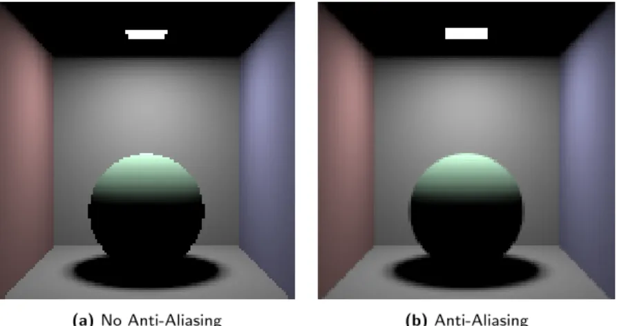
(a)No Anti-Aliasing (b)Anti-Aliasing
Figure 2.5: Direct Illumination. When an image is rendered with only 1 sample per pixel (left), there can be obvious aliasing at the edges. Increasing the number of samples leads to a nicely anti-aliased image (right). Both images rendered with an intentionally small resolution (128×128) to emphasize the aliasing artifacts.
directly from the light sources. Refering to the Equation2.9we can write: Lo(x, ωo) =Le(x, ωo) +
Z
A
fr(x, ωo,Ψ)Le(y,−Ψ)V(x, y)G(x, y)dy (2.27)
whereLo(x, ωo) is determined by the Le of the directly visible surface, but
the integral representing reflected radiance coming from other surface points y takes into account only radiance emitted by those surfaces, not reflected off of them. We can imagine that the camera records only photons that start at a light source and then interact with the scene surfaces at most once.
In the context of ray tracing algorithms, the implementation usually works in the following steps:
1. A ray is shot through the center of a pixel, determining its pointx. 2. The integral is evaluated using Monte Carlo integration, randomly
positioning samples y on the surfaces proportional to their emitted flux. Ray casting is used to evaluate the visibility functionV(x, y). A drawback of this basic approach is that it assumes a constant Lo for
the whole pixel. However, for pixels with a finite extent, this is not true, most notably when the pixel overlaps object boundaries. This results in objectionable aliasing artifacts, such as seen on Figure2.5a.
To reduce the aliasing, we have to take multiple samples for each pixel. The required number depends on the specific scene configuration, but commonly it is between 4 and 256 samples per pixel. To produce Figure2.5b we chose a different method and instead of having a fixed number of samples per pixel, we generate a new unique sample x from the pixel whenever we
(a)Direct Illumination (b)Whitted-style (c)Glossy instead of mirror
Figure 2.6: Direct illumination fails to convey many materials, such as glass and mirror (left). Using the Whitted-style ray tracing, the materials of the two balls become immediatelly obvious (middle). Unfortunately, the approach is not directly applicable to glossy materials (right).
generate a new sampley on a light. This way we can continuously improve the quality until we are satisfied with the result.
2.3.2 Whitted-style Ray Tracing
Figure 2.7: The Whitted-style ray tracing. Rays that encounter glass bifurcate into the reflection and re-fraction directions and recurse until they encounter a non-specular sur-face, or a maximum recursion depth is reached.
One disadvantage of a pure direct illumi-nation solution is that it cannot really con-vey highly specular materials, such as mir-rors and glass (Figure 2.6a). The reason is that only light from a narrow cone of directions contributes to the integral. In the case of a perfect mirror and glass (as introduced in Section 2.1.5), this narrow cone actually becomes infinitely thin and the probability of sampling a pointyon a light such that it would contribute toward Lo is zero.
Turner Whitted [Whitted 1980] in-troduced a simple solution for exactly the case of perfect mirror and glass. The idea is that when the BSDF at the pointx lim-its the integral to a discrete set of
direc-tions from which it can gather the illumination, these direcdirec-tions are explicitly sampled by further rays. For example, when a ray from camera encounters a glass sphere (Figure2.7), where only perfect reflection and refraction di-rections can contribute, the ray bifurcates and continues in both didi-rections. This process is recursively repeated until all the rays reach surfaces that can be directly illuminated. To prevent infinite recursion due to, e.g., perfect internal reflection in glass, a certain maximum recursion depth is usually
enforced, selected such that the effect on the result is minimal (we use max-imum recursion depth of 20).
Using this technique greatly improves visualization of scenes consisting of a combination of mostly diffuse and perfectly specular materials. How-ever, it cannot handle highly glossy surfaces, where contributing illumination can arrive from a narrow but finite cone of directions, as multiple rays are needed to sample this cone (Figure2.6c).
2.3.3 Path Tracing
Both previous techniques solved a simplified version of the rendering equa-tion, as they reduce the fr and Lo terms inside the integral to discrete
distributions, respective emitted radiance. On the other hand, Path Trac-ing, as introduced by Kajiya [Kajiya 1986], is the direct implementation of Equation2.8, repeated here for convenience:
Lo(x, ωo) =Le(x, ωo) +
Z
Ω+
fr(x, ωo, ωi)Lo(h(x, ωi),−ωi) cosθidωi
To solve this recursive equation, we start at the camera and trace a ray through one of the image pixels, same as in the previous algorithms. We evaluateLo at the first intersection pointx with the scene by accumulating
Leand sampling the integral. The integral is sampled by choosing a random
directionωiand tracing a ray in this direction to determine the pointh(x, ωi)
whose Lo will be used in the integral. The process is recursively repeated,
forming apath of rays, withvertices at each interaction with the scene. It is clear that in a closed scene, this algorithm by itself would lead to infinitely long paths. The naive solution would be to artificially limit the path length to a given number of vertices. However, choosing a maximum path length that will provide good results highly depends on the scene. If the path length is too short, it can cause visible artifacts in scenes, e.g., in a scene with many mirror interreflections. If the path length is too long, many of the paths will perform computations with little to no impact on the final result.
A better approach is to used Russian Roulette to probabilistically terminate the paths. It is based on the intuition, that instead of taking 10 random samples we can take only 2, but each of these will have 5× larger impact. More formally, we can write that a samplextaken from a PDFp(x) with a russian roulette probability prr evaluates at prrf(·px()x). The common
choice ofprrin the context of Path Tracing is
R
Ω+fr(x, ωo, ωi)dωi, the albedo
of the material at a given vertex. The intuition is that paths continuing from dark materials will have overall lower contribution to the final result than paths continuing from light materials.
In practice, these methods are often combined, as maximum path length is useful to prevent extremely long recursions in case of scene with
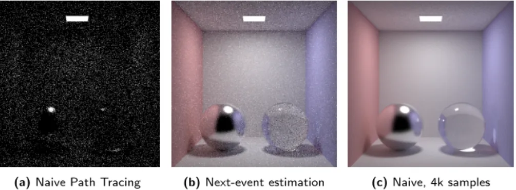
(a)Naive Path Tracing (b)Next-event estimation (c)Naive, 4k samples
Figure 2.8: Naive Path Tracing (left) depends on a path randomly hitting light emitting surfaces, leading to high variance (we used 20 samples per pixel). With next-event estimation (middle), the lights are sampled explicitly leading to a significantly better quality for the same number of samples. Path Tracing without the next-event estimation is still noisy after 4000 samples per pixel (right).
albedos close to, or equal to, one. However, due to the presence of russian roulette, this maximum value does not have a direct impact on performance and can therefore be set sufficiently high (numbers between 20 and 256 are common).
Naive Path Tracing depends only on chance to connect the camera to lights. It is obvious that, as the lights become smaller, the noise increases (Figure2.8a). To improve this, we can stratify our sampling by identifying all light sources in the scene and making explicit connections to them similar to the direct illumination approach. This technique is called next-event estimation and can be formally written as:
Ls(x, ωo) = Z Ω+ fr(x, ωo, ωi)Ls(h(x, ωi),−ωi) cosθidωi (2.28) + Z A fr(x, ωo,Ψ)Le(y,−Ψ)V(x, y)G(x, y)dy
where Ls(x, ω) is radiance scattered from the point x in the direction ω,
and it can be written thatLo(x, ω) =Le(x, ω) +Ls(x, ω). The first integral
of the equation handles light scattered from other surfaces and the second integral light emitted by light sources.
This approach significantly increases the quality of rendering for the same number of camera samples (Figure 2.8b) but still has room for im-provement. Veach and Guibas [Veach and Guibas 1995] propose to use Multiple Importance Sampling (see Section 2.2.3) to combine both tech-niques of connecting to lights. This approach always samples lights through both techniques, i.e., randomly hitting the light and the next-event estima-tion, and combines them using weights that are based on the probability of a given technique finding the contribution such that the technique resulting in higher variance for each given contribution is assigned lower weight,
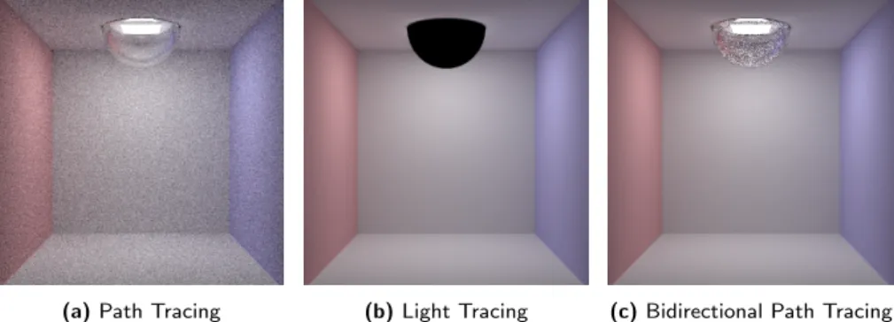
result-(a)Path Tracing (b)Light Tracing (c)Bidirectional Path Tracing
Figure 2.9: Path Tracing with next-event estimation (left) cannot explicitly sample a light behind a fixture. Light Tracing (middle) cannot connect between specular surfaces and pinhole camera, causing the light fixture to appear black. Bidirectional Path Tracing (right) connects camera sub-paths to light sub-paths that already passed through the fixtures, resulting in less noise in the rendering same time (1 second, for all images).
ing in the overall lower variance for the image than if just a single technique was used. We refer the readers to Veach’s thesis [Veach 1997] for details.
2.3.4 Bidirectional Path Tracing
In the previous section we have seen the usefulness of sampling lights ex-plicitly. Bidirectional Path Tracing extends this idea by sampling a full sub-path starting at the light (light sub-path) and connecting the camera sub-path to it.
Unfortunately, in many scenes the light source is enclosed in some kind of glass and metal fixture, making direct connection impossible be-cause the light has to get refracted. In this case, the next-event estimation is effectively removed and the algorithm degenerates into Naive Path Trac-ing (Figure 2.9a). Light Tracing reverses the tracing process, starting at the lights. However, purely specular surfaces appear black (Figure 2.9b) because the probability that the commonly used pinhole camera will lie in the direction of the reflected (or refracted) ray is always zero. Thus, the camera does not receive any radiance from such surfaces.
In Bidirectional Path Tracing both approaches are combined (Fig-ure 2.9c). Furthermore, it allows a direct vertex connection not only be-tween a light sub-path and camera and a camera path and lights, but also between the light and camera sub-path vertices. As this presents multiple ways the camera can be connected to the same light (e.g., the same path constructed from camera or from the light), an extra care has to be taken to not account the light’s contribution multiple times. The common approach is, again, to use Multiple Importance Sampling [Veach 1997,Georgiev 2012,
van Antwerpen 2011a], which automatically assigns higher weight to the more suitable connections.
The common implementation then works in three steps. In the first step, a light sub-path is traced and its vertices are stored. In the second step, a camera sub-path is traced. In the third step, vertices on the light and camera sub-paths are connected, forming several full paths, each of which is properly weighted using Multiple Importance Sampling. A common ap-proach is to not store the first vertex of the light sub-path (i.e., vertex directly on the light) and instead connect each camera sub-path vertex di-rectly to its own, randomly generated, vertex on the light. This removes some correlation, coming from reusing light sub-path vertices, at virtually no additional cost.
While Bidirectional Path Tracing can efficiently capture a large set of paths, it still has problem with specular-diffuse-specular paths, e.g., reflected caustics. The intuition is that connecting through a specular interaction so we arrive at a preselected vertex in the scene (e.g., a light) is generally not possible. To do this we would have to choose only the vertex we want to connect to, but also the exact outgoing direction that will, after reflect-ing/refracting on the specular objects, arrive at this vertex. As this problem can only be solved at a fairly high cost [Jakob and Marschner 2012,Hanika et al. 2015] it is generally recommended to use rendering approaches based on Photon Mapping which we describe in the next section.
2.3.5 (Progressive) Photon Mapping
Figure 2.10: In Bidirectional Path Tracing, the path cannot per-form any vertex connection with-out two consecutive non-specular (green) surfaces, as the specular sur-faces (red) enforce a single outgoing direction.
While Bidirectional Path Tracing (BPT) has a wider set of efficiently handled light transport paths than Path Tracing, some configurations still present problems. The setting on the left side of Figure 2.11a presents one such case. Both the cam-era and the light are covered by per-fectly specular glass, leaving no option to perform any direct vertex connections between the light and camera sub-paths when evaluating direct illumination. As a result, BPT degenerates into Naive Path Tracing for this type of paths. See Fig-ure 2.10 for the schematic view of such configuration. Approaches based on Pho-ton Mapping relax the way paths are con-structed, leading to a better handling of such cases (Figure2.11b).
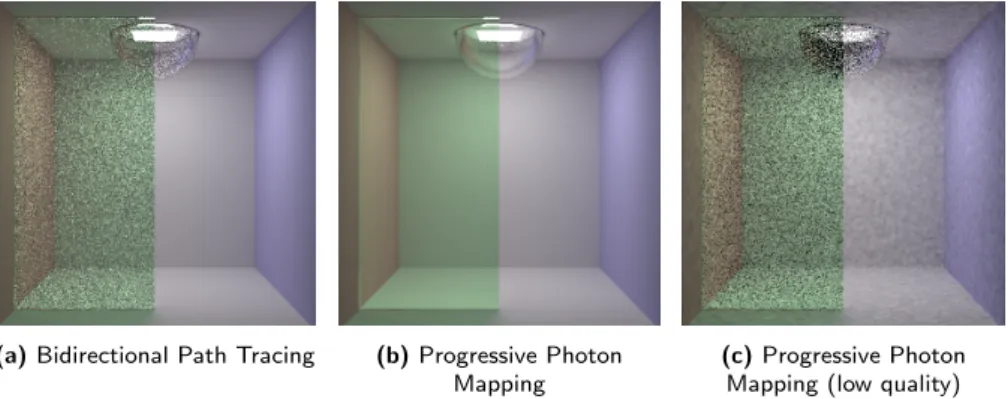
(a)Bidirectional Path Tracing (b)Progressive Photon Mapping
(c)Progressive Photon Mapping (low quality)
Figure 2.11: A Cornell Box with the left side viewed through a green tinted glass, and the light source inside a glass fixture. Bidirectional Path Tracing (left) degenerates into Naive Path Tracing when surfaces are illuminated through glass as well as seen through glass. Progressive Photon Mapping (middle) can handle such illumination well, at the cost of introducing bias and a lower order of convergence. A low quality Progressive Photon Mapping image (right) shows the splotchy artifacts typical for this rendering technique.
different view on global illumination. It is a two-pass algorithm where, in the first pass of the method photons are emitted from light sources and deposited onto surfaces, storing their position, energy, and incoming direction (for BRDF evaluation). In the second pass, camera sub-paths are traced and the photon density is estimated in the neighborhood of their first non-specular vertex (gather point). The density estimation is usually facilitated by finding theknearest photons (typically 20-50), using a k-Nearest Neighbors (k-NN) search [Hey and Purgathofer 2002]. The outgoing radiance is computed as:
Lo=Le+ 1 πr2 k−1 X j=1 fr(x, ωo, ωi,pj)kr(dj)∆Φpj (2.29)
wherexis the position of the gather point,fr is the BRDF at this position,
r is the radius of circle in which our k photons lie, ωi,pj is the incoming
direction of the photon pj, kr is a normalized and scaled kernel weight
function1, dj is the distance of the photon from x, and ∆Φpj is the flux
it carries. The intuitive reason why onlyk−1 photons are used is that the kthphoton, at the very border of our search circle, does not contribute all of its energy into our search area. Please see [Garc´ıa et al. 2012] for rigorous derivation.
A key difference from the path-based methods is that the paths are not evaluated exactly. During the density estimation, the end points of light sub-paths (photons) are moved to the gather point position, even in
1
We use the simplest, cylindrical, kernel, and the kr is therefore constant inside the
cases where the nature of light sub-path would not allow this, i.e., if the previous vertex on the sub-path was specular and did not allow other di-rections (Figure 2.12). While blurring of light transport introduces a new type of error in ourLo estimate, bias, it also allows for a better handling of
specular-diffuse-specular type of paths than Bidirectional Path Tracing.
Figure 2.12: Photon Mapping ap-proaches allow “merging” of path vertices on non-specular (green) sur-faces, allowing for use of bidirec-tional methods even where BPT does not.
Hachisuka et al. [2008] propose Pro-gressive Photon Mapping, a Photon Map-ping based method that, while biased, is consistent, i.e., in the limit it converges to the ground truth solution. In the first pass of the algorithm, camera sub-paths are traced and the gather points are stored. The gather points include all the informa-tion required to evaluate the BRDF at the point, as well as the current density es-timation radius r, the total accumulated flux and the number of photons accumu-lated so far. In the subsequent passes, photons are traced from lights. Photons are not stored but, instead, immediately contribute to all gather points in whose
radius r they fall. After each such pass, the radius r of each gather point is reduced using the collected statistics in such a way that the radius be-comes zero in the limit. This approach has been expanded to Stochastic Progressive Photon Mapping [Hachisuka and Jensen 2009] to allow chang-ing the gather points between photon passes (e.g., for anti-aliaschang-ing or depth of field). Knaus and Zwicker [Knaus and Zwicker 2011] change the formula-tion to remove the requirement for per-pixel statistics. Vorba [Vorba 2011] introduces Progressive Bidirectional Photon Mapping, where a full camera sub-path is traced, density estimation is performed at each non-specular vertex of the path and the results are combined using Multiple Importance Sampling.
Georgiev et al. [2012] and Hachisuka et al. [2012] concurrently refor-mulate the Photon Mapping in the context of path-based methods, allowing combining of Progressive (Bidirectional) Photon Mapping with Bidirectional Path Tracing are using Multiple Importance Sampling (MIS) into a novel algorithm, namedVertex Connection and Merging by Georgiev andUnified Path Sampling by Hachisuka. This work uses the name Vertex Connection and Merging, as the author participated on the [Georgiev et al. 2012] paper, but the names are completely interchangeable. For derivation of the MIS weights, see [Georgiev 2012].