GLOBAL OPTIMIZATION OF COMPUTATIONALLY
EXPENSIVE BLACKBOX PROBLEMS USING RADIAL
BASIS FUNCTIONS
A Dissertation
Presented to the Faculty of the Graduate School of Cornell University
in Partial Fulfillment of the Requirements for the Degree of Doctor of Philosophy
by
Tipaluck Krityakierne August 2014
c
!2014 Tipaluck Krityakierne ALL RIGHTS RESERVED
GLOBAL OPTIMIZATION OF COMPUTATIONALLY EXPENSIVE BLACKBOX PROBLEMS USING RADIAL BASIS FUNCTIONS
Tipaluck Krityakierne, Ph.D. Cornell University 2014
Three derivative-free global optimization methods are developed based on radial basis func-tions (RBFs) for computationally expensive blackbox simulation models. First, we develop a multistart global optimization method, called SOMS (SurrOgate MultiStart). SOMS uses an RBF surrogate model to approximate the objective function in order to reduce the number of function evaluations necessary to identify the most promising points from which each non-linear programming local search is started. We show that SOMS detects any local minimum within a finite number of iterations almost surely. The numerical results show that SOMS performs favorably in comparison to alternative methods and that the surrogate approach saves a significant number of computationally expensive function evaluations.
In the second part of this work, we introduce PADS (PArallel Dynamic coordinate search with Surrogates), which is a surrogate-based global optimization framework for high-dimensional expensive blackbox functions. In each parallel iteration of PADS, multiple points are selected from a large set of candidate points that are generated by perturbing only a subset of the coordinates of the current best solution. The selected points are then eval-uated in parallel with up to 16 parallel processors. We show that PADS converges to the global optimum with probability 1. We develop two versions, PADS1 and PADS2, which use different underlying distributions to generate candidate points. We show that PADS1 and PADS2 are able to find better solutions more efficiently compared to alternative methods, with PADS1 performing even better than PADS2 in problems up to 200 dimensions.
In the final part of this dissertation, we develop an effective new parallel surrogate global optimization method called SOP (Surrogate Optimization with Pareto center selection). The
search mechanism of SOP incorporates bi-objective optimization, tabu search, and surrogate assisted local search, which exploits the information from the already evaluated points, for selecting a large number of new evaluation points. The newly selected points are evaluated in parallel, and hence a significant reduction in wall-clock time can be achieved. We give sufficient conditions for almost sure convergence of SOP. The results of our numerical exper-iments show that SOP performs very well compared to alternative parallel surrogate model algorithms with 8 and 32 processors obtaining superlinear speedup on some test problems.
BIOGRAPHICAL SKETCH
Tipaluck Krityakierne was born as a second daughter to a Thai father and a Singaporean mother. Tipaluck spent several years of her childhood in Tokyo before moving back to Bangkok, Thailand, when she was about five years old. She grew up in a multicultural and multilingual environment.
From pre-school to high school, she attended Satit Prasarnmit Demonstration School. Funded by the Office of the Higher Education Commission of Thailand, she majored in Mathematics at Chulalongkorn University. After graduating as the top ranked student in her program, she received two prestigious fellowships: the Anandamahidol Foundation Schol-arship under the patronage of H.M. the King of Thailand and the Fulbright fellowship. These two fellowships gave her an opportunity to come to the US in 2007 to pursue her Ph.D. in Applied Mathematics at Cornell University.
Tipaluck received her Master of Science degree in Applied Mathematics in 2011 and received her Ph.D. degree in August 2014. She will be joining the Institute of Mathematical Statistics and Actuarial Science at University of Bern, Switzerland in September 2014 as a Swiss Government Excellence Postdoctoral Scholar.
ACKNOWLEDGEMENTS
This dissertation is the end of a long journey that began 8544.73 miles away from home. It was made possible through the support of many people, to whom I now have the pleasure of expressing my appreciation and gratitude.
First and foremost, I would like to express my deepest gratitude to my advisor Prof. Christine Shoemaker. Her support and encouraging guidance have been instrumental in shaping this work and helping me reach my destination. I would also like to thank Prof. Peter Frazier and Prof. Michael Nussbaum, who served on my dissertation committee, for their help over the years. I offer my thanks, as well, to Prof. Tapan Mitra for introducing me to the world of mathematical economics. Although this part of my work was not incorporated into this dissertation, it has been a tremendous learning experience for me.
I am grateful to my fellow students at Center for Applied Mathematics for their good humor and good conversation, all of which have made our office a pleasant place to work. I especially thank Adam Chacon for helping with parallel programming, as well as for sharing the difficult and the good moments during this journey with me. To Huimei Delgado, I thank her for all the support and friendship she has given me. I will always remember the endless hours we spent doing homework assignments and debugging code together. I thank Mathav Murugan for his useful suggestions and for checking many of my mathematical proofs. I am also grateful to Yilun Wang, who gave me programming advice during the initial stage of this work. I owe special thanks to Juliane Müller for her valuable suggestions and comments, and her encouragement and willingness to proofread countless pages of this dissertation.
I thank Prapanpong Pongsriiam and Santi Tasena, my academic brothers, who took their time and patience to help me understand many mathematics materials. Their explanations in Thai made it much easier to understand difficult mathematical concepts. I am grateful, as well, to my former college professors: Prof. Patanee Udomkavanich, Prof. Wicharn Lewkeeratiyutkul, and Prof. Kittipat Wong for their helpful advice and being supportive for the past ten years.
For all their love and support, I offer special thanks to my extended family and friends in Thailand, Singapore, Japan, and here in the US. While there are too many to name, I would especially like to thank all my Thai friends at Cornell who have shared part of this journey with me. I have also enjoyed the warm friendship of my Japanese teacher, Naomi Larson, and her family, Kent and Komi. Thank you for always providing the support that I needed.
I would like to thank my dance instructors, Byron Suber and Jumay Chu, for providing enjoyable and challenging classes and unforgettable performance opportunities. Whenever I walk into the ballet studio, I feel the homey atmosphere that releases me from the pressures of research work. All my dance friends at the Department of Performing & Media Arts also play important part of my life at Cornell. This journey would have been all the more difficult were it not for their warm and loving friendship over the years.
Sahoko Ichikawa, thank you for being the best roommate anyone could ask for. I am very grateful for your helping hand, for the healthy and delicious food you cooked me, and for all you have done to support me during all these years. My sincerest thanks to ot¯osan and ok¯asan, Tadao and Yoriko Ichikawa, who have been very supportive and caring. Thank you for being my surrogate family in Japan, and for walking through this journey with me. Itu mo arigat¯o gozaimasu.
Most importantly, I would like to express my deepest appreciation to my Krityakierne family in Thailand: my mother, Nancy, my father, Varaj, my sister, Tirolarn, and my beloved brother, Kousak, for their unconditional love and care, as well as their boundless support in every respect. I appreciate more than I can say all that they have done to support me throughout the course of this long journey.
Finally, I am exceptionally grateful for support from Anandamahidol Foundation Schol-arship under the patronage of H.M. the King of Thailand and the Fulbright Fellowship. I am thankful for various teaching assistantships with Cornell’s Center for Applied Mathematics and research assistantships with the School of Civil and Environmental Engineering through
grants from NSF to C. Shoemaker CISE-1116298 and from DOE SciDAC to N. Mahowald and C. Shoemaker DE-SC0006791.
Table of Contents
Biographical Sketch . . . iii
Dedication . . . iv
Acknowledgements . . . v
Table of Contents . . . viii
List of Tables . . . xi
List of Figures . . . xii
List of Algorithms . . . xiv
1 Introduction 1 2 Surrogate MultiStart Algorithm for Nonlinear Programming Problems 8 2.1 Introduction . . . 8
2.2 SOMS: SurrOgate MultiStart . . . 13
2.2.1 Improving the Accuracy of the Initial Response Surface . . . 15
2.2.2 A Cubic Radial Basis Function Model . . . 16
2.2.3 Addition of Uniformly Selected Points . . . 18
2.3 Theoretical Properties of SOMS . . . 18
2.4 Multistart Methods in the Numerical Comparison . . . 24
2.5 Numerical Experiments . . . 29
2.5.1 Experimental Setup . . . 29
2.5.2 Performance Measure . . . 31
2.6 Numerical Experiments for Dixon-Szegö Test Functions . . . 32
2.6.1 Discussion on the Dixon-Szegö Test Results . . . 35
2.6.2 Parameters of MATLAB’s GlobalSearch solver . . . 36
2.6.3 Influence of the Uniformly Selected Point in SOMS . . . 37
2.7 Wavy Test Functions . . . 37
2.7.1 Creating Wavy Test Functions for Optimization . . . 40
2.7.2 Underlying Function . . . 41
2.8 Numerical Experiments of Wavy Test Functions . . . 44
2.8.1 Wavy Test Functions . . . 45
2.8.2 Results for Low-dimensional Wavy Test Functions . . . 46
2.8.3 Results for High-dimensional Schoen and SchoenWavy . . . 50
2.8.4 Solution Accuracy of SOMS . . . 54
3 Parallel Dynamic Coordinate Search with Surrogates 57
3.1 Introduction . . . 57
3.1.1 Related Work . . . 58
3.1.2 Stochastic Response Surface (SRS) Framework . . . 60
3.1.3 Main Contributions . . . 60
3.2 PADS Framework . . . 62
3.2.1 PADS(J) Description . . . 63
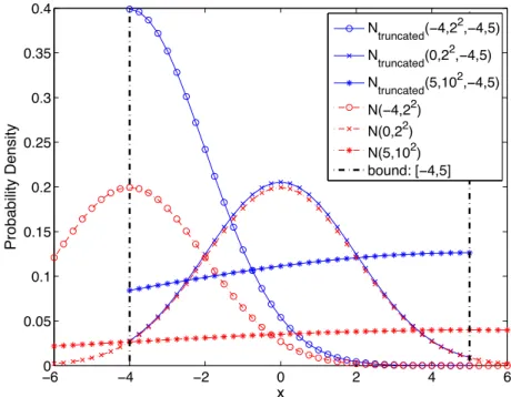
3.2.2 Truncated Gaussian Distribution . . . 70
3.3 Convergence of PADS Methods . . . 72
3.4 Computational Experiments . . . 77
3.4.1 Test Problems . . . 77
3.4.2 Alternative Global Optimization Methods . . . 77
3.4.3 Experimental Setup . . . 83
3.5 Numerical Results and Discussion . . . 84
3.5.1 Performance Measurement Setup . . . 85
3.5.2 Comparison with Alternative Methods . . . 86
3.5.3 Analysis of PADS1(J) . . . 97
3.6 Conclusions . . . 111
4 Surrogate Optimization with Pareto Center Selection 115 4.1 Introduction . . . 115
4.1.1 Literature Review . . . 116
4.1.2 Differences between SOP and Previous Algorithms . . . 118
4.2 Background . . . 120
4.2.1 General Framework for Surrogate Model Based Optimization . . . . 120
4.2.2 Bi-objective Optimization . . . 121
4.3 SOP: Surrogate Optimization with Pareto center selection . . . 124
4.3.1 Non-dominated Sorting (NDS) and P Center Selection . . . 132
4.3.2 Example of Tabu Structure . . . 136
4.3.3 Local Candidate Search . . . 138
4.4 Convergence of nSOP . . . 140
4.5 Numerical Experiments . . . 145
4.5.1 Alternative Optimization Algorithms . . . 145
4.5.2 Experimental Setup . . . 147
4.5.3 Test Functions . . . 148
4.5.4 Progress Curve in Wall-clock Time . . . 148
4.5.5 Experimental Results and Discussion . . . 149
4.5.6 Groundwater Bioremediation Problem . . . 156
4.5.7 Relative Speedup . . . 159
4.6 Conclusions . . . 163
5 Conclusions 165 5.1 A Surrogate Multistart Framework . . . 165
5.2 Surrogate Models for HEB Problems . . . 166 5.3 Surrogate Model Algorithm with Bi-objective Point Selection Optimization . 166
5.4 Future Work . . . 167
List of Tables
1.1 Key features of algorithms developed in this thesis . . . 7
2.1 Algorithm parameters for SOMS and MLSL . . . 30
2.2 Algorithm parameters for GlobalSearch . . . 31
2.3 Dixon-Szegö testbed . . . 32
2.4 Results for Dixon-Szegö . . . 33
2.5 One-tailed t-test results for Dixon-Szegö test functions. . . 36
2.6 Results of GlobalSearch with different algorithm parameters . . . 38
2.7 Results of SOMS with and without adding a uniform point . . . 39
2.8 Low-dimensional wavy test functions . . . 45
2.9 High-dimensional wavy test functions . . . 46
2.10 Results for low-dimensional wavy test functions . . . 48
2.11 One-tailed t-test results for low-dimensional wavy test functions. . . 50
2.12 Results for high-dimensional wavy test functions . . . 52
2.13 One-tailed t-test results for high-dimensional wavy test functions. . . 54
3.1 Test problems used in the experiments . . . 78
3.2 Parameter values for PADS and LMSRBF . . . 84
3.3 α-levels . . . 108
3.4 The relative distance (%) from α6 to y∗ 1 . . . 111
4.1 Example of a tabu structure . . . 138
4.2 Parameter values for SOP . . . 147
4.3 Benchmark functions for SOP . . . 148
4.4 Results for BBOB testbed using 8 processors . . . 154
4.5 The collective t-test results for P=8 . . . 155
4.6 Results for BBOB testbed using 32 processors . . . 155
4.7 The collective t-test results for P=32 . . . 156
4.8 Results for GWB12D after 60 hours . . . 159
4.9 α-levels . . . 161
List of Figures
1.1 Example of an RBF surrogate model fit to sample data . . . 3
1.2 Surrogate-based global optimization framework . . . 3
2.1 Box plots for Dixon-Szegö test functions . . . 34
2.2 Wavy-1D . . . 39
2.3 easySquareWavy . . . 41
2.4 LagrangeWavy2 . . . 43
2.5 SchoenWavy-2D . . . 44
2.6 Box plots for low-dimensional wavy test functions . . . 49
2.7 Box plots for high-dimensional wavy test functions . . . 53
2.8 Stochastic RBF result for LagrangeWavy2 . . . 55
3.1 Probability of selecting a variable of xbest for perturbation . . . 65
3.2 Pseudocode Perturb_x . . . 66
3.3 Candidate points for various values of pselect . . . 67
3.4 Pseudocode Select_J_Evaluation_Points . . . 69
3.5 Pseudocode Adjust_Step_Size . . . 70
3.6 Comparison of Gaussian and truncated Gaussian distributions . . . 71
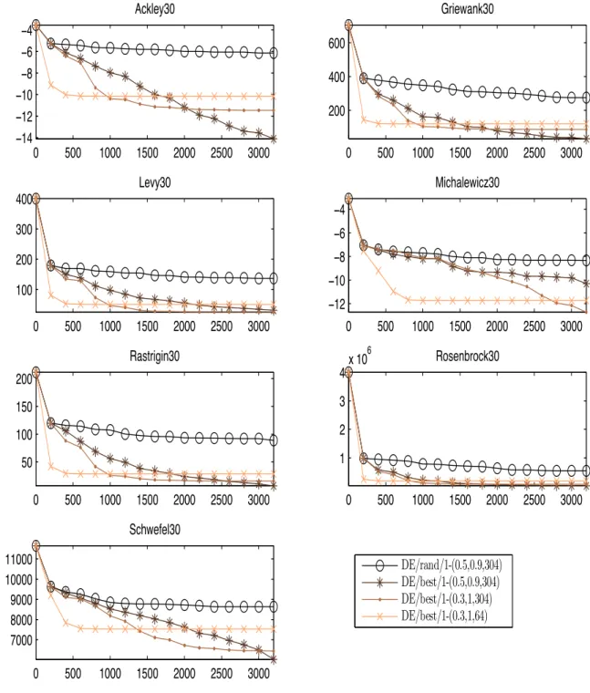
3.7 Results of DE for 30-dimensional problems . . . 81
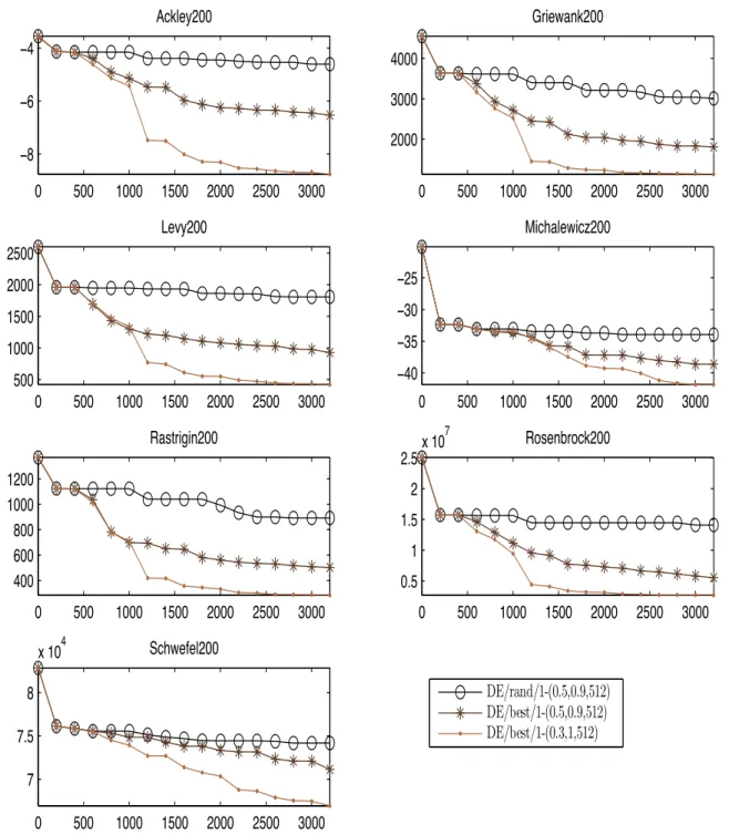
3.8 Results of DE for 200-dimensional problems . . . 82
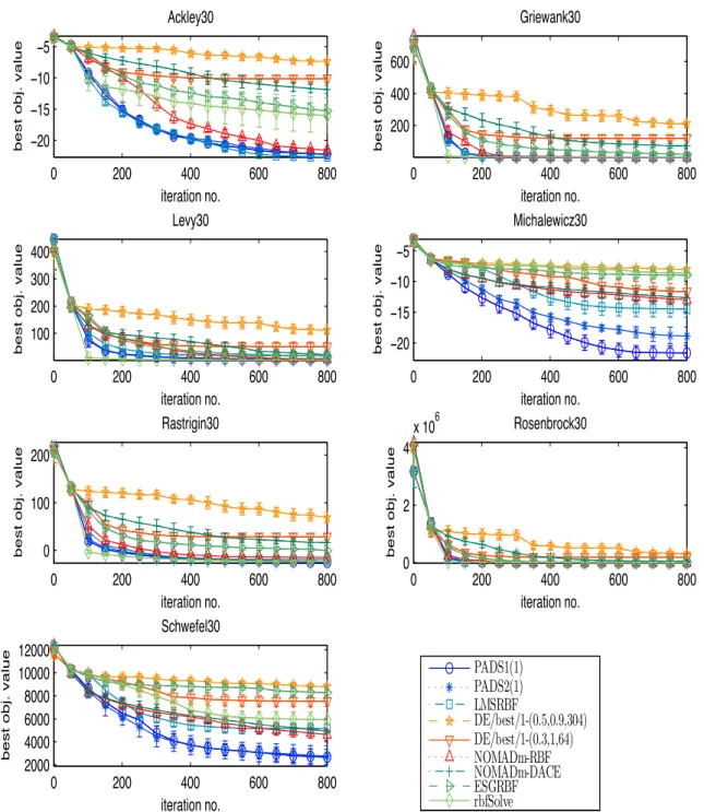
3.9 Comparison of serial algorithms for 30-dimensional problems . . . 88
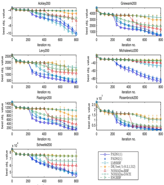
3.10 Comparison of serial algorithms for 200-dimensional problems . . . 89
3.11 Comparison when using 4 processors for 30-dimensional problems . . . 90
3.12 Comparison when using 4 processors for 200-dimensional problems . . . 91
3.13 Comparison when using 8 processors for 30-dimensional problems . . . 93
3.14 Comparison when using 8 processors for 200-dimensional problems . . . 94
3.15 Comparison when using 16 processors for 30-dimensional problems . . . 95
3.16 Comparison when using 16 processors for 200-dimensional problems . . . 96
3.17 Cumulative indices when using 1 processor . . . 98
3.18 Cumulative indices when using 4 processors . . . 99
3.19 Cumulative indices when using 8 processors . . . 100
3.20 Cumulative indices when using 16 processors . . . 101
3.21 Progress plots of PADS1 for 30-dimensional problems . . . 103
3.22 Progress plots of PADS1 for 200-dimensional problems . . . 104
3.23 α-Speedup(J) of PADS1 for 30-dimensional problems . . . 109
3.25 α-Work Ratio(J) of PADS1 for 30-dimensional problems . . . 112
3.26 α-Work Ratio(J) of PADS1 for 200-dimensional problems . . . 113
4.1 A two-objective space and the corresponding non-dominated fronts . . . 122
4.2 Hypervolume . . . 123 4.3 Pseudocode select_P_indices . . . 128 4.4 Pseudocode hypervol_improv_indc . . . 129 4.5 Hypervolume improvement . . . 130 4.6 Pseudocode update . . . 132 4.7 Pseudocode non_dom_sorting . . . 134 4.8 Pseudocode P_centers_sel . . . 135
4.9 Example of center selection . . . 136
4.10 Pseudocode local_candidate_search . . . 139
4.11 Progress curves for BBOB when using 8 processors . . . 151
4.12 Progress curves for BBOB when using 32 processors . . . 152
4.13 Progress curves for BBOB (combined) . . . 153
List of Algorithms
2.1 Multistart Procedure . . . 9
2.2 SurrOgate MultiStart (SOMS). . . 14
2.3 Multi Level Single Linkage (MLSL) . . . 25
2.4 MATLAB’s MultiStart (MS) . . . 25
2.5 MATLAB’s GlobalSearch (GS) . . . 26
2.6 GLOBAL (GLOB) . . . 27
3.1 Stochastic Response Surface (SRS) . . . 61
3.2 PArallel Dynamic coordinate search with Surrogates (PADS) . . . 64
4.1 General framework: P surrogate-based optimization . . . 120
Chapter 1
Introduction
In this dissertation, we consider a real-valued global optimization problem of the form:
min
x∈Df(x) (1.1)
where D ={lb≤x≤ub} ⊂Rd. Here, lb and ub are the lower and upper variable bounds,
respectively, and f(x)is a continuous objective function with the following characteristics: 1. blackbox;
2. computationally expensive;
3. non-differentiable or its gradient is computationally intractable; 4. multimodal.
While these three properties are very common in real-world engineering design problems, conventional optimization methods such as SQP [79], for example, are often not applica-ble because of the following reasons. For complex simulation models, obtaining accurate derivatives can be infeasible or computationally very expensive. Due to this lack of gradient information, gradient-based optimization algorithms such as the steepest descent method or the conjugate gradient method [11, 23] cannot be used. In addition, heuristic methods
[52, 82] such as simulated annealing, genetic algorithms or tabu search generally require too many expensive function evaluations to converge and are therefore not efficient.
As a result, in recent years, an increasing number of algorithms that incorporate surrogate models (also known as response surfaces or metamodels) have been proposed to efficiently solve the class of optimization problems that have objective functions with the characteristics described above. In surrogate model based optimization, the computationally expensive objective function is approximated with an inexpensive surface. An auxiliary optimization problem on this surrogate surface is solved in each iteration to determine the next point at which the true objective function is evaluated. The new data is used to update the surrogate surface, and thus it is iteratively refined. Several popular response surface models such as radial basis functions (RBFs), kriging, polynomials, support vector regression, and multivariate adaptive regression splines (MARS) have been used in optimization [25, 40, 41, 42, 56, 57, 61, 68, 78, 109, 122]. A detailed review of surrogates used in engineering design optimization can be found in [122]. In this dissertation we use RBFs because these models have been shown to generally perform better than the alternative models [77].
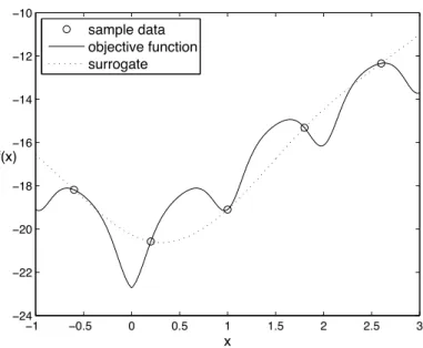
An example of an RBF surrogate is given in Figure 1.1. Five points at which we know the objective function value (marked by ◦) are used to fit the surrogate. The dotted line is the constructed RBF surrogate. The solid line is the true objective function, which is in practice unknown.
Most surrogate-based global optimization algorithms follow the framework given in Figure 1.2. The algorithm starts by creating an initial experimental design at which the costly objective function is evaluated. In each iteration of the algorithm the surrogate model is fit to the data. The surrogate is then used (within the algorithm’s specific optimization strategy) to select xk for the next expensive function evaluation, and if the stopping criteria
−1 −0.5 0 0.5 1 1.5 2 2.5 3 −24 −22 −20 −18 −16 −14 −12 −10 x f(x) sample data objective function surrogate
Figure 1.1: Example of an RBF surrogate model fit to sample data
0: initial design 1: build surrogate 2: optimization on surrogate; output xk 3: do costly evaluation: f(xk) 5: update surrogate 4: check stopping criteria stop k= 1 no k=k+ 1 yes
The aims of this dissertation are to design and implement RBF based global optimization algorithms that are able to achieve a fast decrease in function value with respect to the number of function evaluations (for serial algorithms) or the wall-clock time (for parallel algorithms). The questions investigated and the contributions of this dissertation can be summarized as follows.
1. We investigate the use of RBFs within a multistart local search optimization framework. 2. We investigate the performance of different surrogate-based (both serial and parallel) global optimization algorithms for high dimensional problems (up to 200 dimensions). 3. We investigate the performance of different RBF based algorithms in a parallel opti-mization framework when a large number of function evaluations are done simultane-ously.
To address the first aspect, in Chapter 2, we propose SOMS: SurrOgate MultiStart algo-rithm for global optimization. SOMS is an efficient surrogate-based multistart algorithm, which is used in combination with a nonlinear local optimization routine to find the global minimum of the computationally expensive multimodal objective function. In practice, lo-cal optimization methods are often applied to complex nonlinear optimization problems. However, local optimization algorithms generally stop at a local minimum, and hence the global minimum may be missed. While methods based on multistart can also be helpful for computationally expensive functions when identifying other good local minima (besides the global minimum) is useful, existing multistart algorithms are inefficient because a large number of sample points have to be evaluated on the expensive function before a starting point for a local search can be located. This motivates the investigation of the use of re-sponse surface models within the multistart framework to help reduce the number of function evaluations necessary to identify the most promising points from which to start each non-linear local solver. SOMS’s numerical results are compared with four well-known methods, namely, Multi Level Single Linkage (MLSL) [59, 60], MATLAB’s MultiStart, MATLAB’s
GlobalSearch [119], and GLOBAL [30]. The numerical results indicate that SOMS performs favorably in comparison to alternative methods. Theoretical properties of SOMS similar to those possessed by MLSL are also verified.
Because searching in high-dimensional spaces (with several hundred dimensions) unavoid-ably requires a large number of function evaluations (“curse of dimensionality”), solving a class of HEB (High-dimensional, Expensive, and Blackbox) [106] problem with a serial al-gorithm can be extremely time-consuming (due to both the computational expense of a single function evaluation and the optimization algorithm’s own computational overhead). In Chapter 3, we therefore develop and implement PADS (PArallel Dynamic coordinate search withSurrogates), which is a surrogate-based global optimization framework for high-dimensional expensive blackbox functions. PADS selects the next evaluation point from a set of candidate points that are obtained by perturbing only a subset of the coordinates of the current best solution, which is the key idea proposed in DDS [115] and was recently empirically proven to be very effective especially when the problem dimension is very high (200 variables) [97]. In PADS, multiple expensive function evaluation points are evaluated in each iteration, i.e. the output xk in the framework shown in Figure 1.2 is replaced by
!
x(1k), ..., x(Jk)", a set of J selected points for simultaneously evaluating the objective
func-tion.
In addition, different underlying distributions to generate candidate points for next func-tion evaluafunc-tion points within Step 2 of Figure 1.2 will also be investigated. A practical implementation that follows the PADS framework is described and several numerical re-sults are illustrated and compared to alternative methods including DYCORS [97], MADS [1, 2, 9, 65, 67], Differential Evolution [113], ParESGRBF [91, 107], ParLMSRBF [95, 96], as well as TOMLAB’s rbfSolve [15, 50]. The results demonstrate that PADS makes fast progress towards the best possible solution given a limited computational budget and is well suited for very high-dimensional problem. Finally, we also provide convergence conditions and show that PADS converges to the global optimum with probability 1.
When simulations are computationally expensive, one needs to terminate the algorithm after a certain amount of wall-clock time, e.g. 100 hours. Therefore, for serial algorithms (one function evaluation is done in each iteration), the algorithm might be able to do only few hundred evaluations before termination. This inevitably affects the quality of the final solution. Parallel computing technologies make it possible to solve computationally expensive global optimization problems that cannot be solved otherwise by a serial algorithm. With more points simulated per iteration, one would expect that the algorithm converges within fewer iterations. This is, however, not always the case. The challenge, therefore, becomes how to effectively select many points for simultaneous evaluations.
In Chapter 4, we propose a new method, SOP (Surrogate Optimization Pareto center selection). The search mechanism of the algorithm incorporates bi-objective search, tabu search, and surrogate assisted local search. SOP evaluates multiple points and uses the data from all of these evaluations to update the surrogate model in each iteration. Thus, the number of iterations, and hence the wall-clock time, is reduced as opposed to the total number of simulations. SOP differs from the previous method of Regis and Shoemaker [95, 96, 97] in that the search center used to generate candidate points for the next function evaluation points is not always the best point. This contrasts also with the approach used in PADS. To manage the trade-off between exploration and exploitation, bi-objective optimization over a finite set of already evaluated points is used to select the search centers, where one objective is the function value, and the other objective is the minimum distance from all other evaluated points.
There are no existing surrogate global optimization algorithms that select a large number of evaluation points in each iteration. For example, the maximum number of points used in [14], [96], and [120] were 5, 8, and 10 points, respectively. We have tested SOP with up to 64 simulated points per iteration. SOP can do many expensive objective function evaluations simultaneously which greatly reduces wall-clock time. We compare SOP with two other RBF methods, namely, Parallel Stochastic RBF [96] and ESGRBF [91, 107] on the
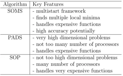
Table 1.1: Key features of algorithms developed in this thesis Algorithm Key Features
SOMS - multistart framework - finds multiple local minima - handles expensive functions - high accuracy potentially PADS - very high dimensional problems
- not too many number of processors - handles expensive functions
SOP - not too high dimensional problems - many number of processors
- handles very expensive functions
Real-Parameter Black-Box Optimization Benchmarking (BBOB) problems [47]. In addition to the BBOB testbed, the algorithms are also compared on an application problem that deals with groundwater bioremediation where the goal is to minimize the cost of the cleanup of contaminated groundwater subject to a contamination constraint. Sufficient conditions for the convergence of SOP will also be discussed.
In summary, this dissertation presents novel algorithms that can quickly identify near optimal solutions of computationally expensive blackbox functions when a relatively small number of function evaluations or a relatively short wall-clock time is allowable. The key features of each of the three algorithms are summarized in Table 1.1. Our algorithms are empirically validated on a broad set of benchmark problems. Finally, under some conditions, almost sure convergence for algorithms that follow the SOMS, PADS and SOP frameworks is proved.
Chapter 2
Surrogate MultiStart Algorithm for
Nonlinear Programming Problems
2.1
Introduction
Several stochastic methods have been developed in the past to solve the problem in Eq. (1.1) for blackbox functions. When the objective function is in addition expensive, methods that use surrogate models in place of the objective function were shown to be the most successful [45, 56, 57, 95, 97, 98]. A surrogate-based optimization approach is designed to approximate the computationally expensive objective function. During the optimization search process, the surrogate is updated each time the exact objective function is evaluated, while the search is moving towards the global optima.
While all these methods are developed as stand-alone global optimization algorithms, in this work we are adopting the method based on a multistart framework (see Algorithm 2.1). Here, the term “multistart” will refer to a procedure that (in each iteration) selects a new variable vector which is used as starting a guess for a local optimization algorithm, for example, Sequential Quadratic Programming. Local optimization algorithms generally stop at local optima and may thus not be able to detect the global optimum. The multistart
Algorithm 2.1 Multistart Procedure 1. Set j = 0
2. While (Stopping condition is not satisfied) (a) j =j + 1
(b) (Global Phase) Select a new decision variable xj based on some scheme.
(c) (Local Phase) Apply a local optimization algorithm A to improve xj. Let x#j be
the solution obtained.
(d) Update the best local minimum found so far. End
Output: All the local minima found
approach allows to continue the search globally, and therefore it is possible to escape from local optima.
The starting points for the local optimizations in the multistart algorithm have to be chosen carefully in order to avoid repeated convergence to the same local minimum. Different multistart techniques based on clustering were therefore proposed in order to avoid this inefficiency [10, 20, 58, 59, 114, 116, 117, 118].
This multistart approach is very useful since there are numerous applications of local optimization methods to complex nonlinear simulations for which there is no guarantee that there is only a single local minimum. This includes PDE constrained optimization where the simulation is solving a system of partial differential equations (e.g. [13]). However, in some cases, years have gone into setting up the interface between the local optimizer and the complex simulation model. Interfacing a multistart method with the existing pairing of a local optimizer and a complex simulation model can be much easier than it would be to build a new interface between a stand-alone global optimization method and the complex simulation model. Moreover, methods based on multistart can also be helpful for computationally expensive functions when identifying other good local minima besides the global minimum is of benefit, for example, when the practical implementation of the
globally optimal solution is much more difficult or time consuming than the implementation of a suboptimal solution.
Multi Level Single Linkage (MLSL) [59, 60] developed by Rinnooy Kan and Timmer in 1987 is one of the most classical and widely used linkage methods. Some other methods based on linkage methods are, for example, Topographical Multilevel Single Linkage [6] and Random Linkage [70]. See also [19, 103] for a brief summary of other linkage methods. In MLSL, the local optimization algorithm starts from selected sample points for which no other sample points with better objective function values are located within a critical distance. See Algorithm 2.3 in Section 2.4 for a brief review of MLSL. In 1988, Csendes [29] introduced a clustering method called GLOBAL based on Boender’s algorithm [20]. In 2008, Csendes et al. modified the previous GLOBAL in some places to achieve higher efficiency and reliability [30]. A brief description of this algorithm is presented in Algorithm 2.6, Section 2.4. Another recent well-known multistart method that is based on scatter search is OptQuest/NLP multistart method [119]. The starting points are generated by a scatter-search algorithm and non-promising starting points (derived from the objective function value) are deleted. The method is available in MATLAB’s Optimization Toolbox under the name GlobalSearch solver (Algorithm 2.5, Section 2.4). MATLAB’s Optimization Toolbox also offers another multistart method, called MultiStart. MATLAB’s MultiStart (Algorithm 2.4, Section 2.4) is simply a multistart algorithm that starts a local solver from every point (either uniformly generated or user-supplied) without estimating whether the point is likely to lead to a new and improved solution. All these methods follow the multistart framework given in Algorithm 2.1.
Due to highly nonlinear and multimodal characteristics of the likelihood function, uncer-tainty quantification for computationally expensive models can be very difficult to handle. Espinet [37] uses MLSL based global solver (coupled with ORBIT [124, 125]) to accurately define the high posterior density region of SOARS. SOARS [16, 17, 18] is a recently de-veloped method that can produce a sample of the posterior distributions of selected input
parameters in a computationally efficient way for given monitoring data. Unlike traditional MCMC, SOARS uses a surrogate to approximate the likelihood. Espinet [37] reports that using MLSL coupled with the local optimizer ORBIT is more efficient than alternative mul-tistart methods for the examined carbon sequestration application. He was able to decrease the necessary number of evaluations by a factor of twenty while obtaining accurate estimates of the posterior densities (i.e. they were very close to the posterior densities computed with MCMC analysis of the computationally expensive likelihood function without surrogates or optimization). This result is significant because many objective functions/likelihood func-tions are expensive to evaluate at each possible parameter value so it is not feasible to do the tens of thousands of function evaluations typically required in traditional MCMC. Hence, ef-ficient multistart methods are applicable to uncertainty quantification problems in parameter calibration.
For complex simulation models, getting accurate derivatives can be infeasible or compu-tationally very expensive. For commercial software, source code is in general not available, and thus automatic differentiation cannot be used. In practice, none of these multistart methods require derivatives, and therefore if coupled with derivative-free local search meth-ods such as NEWUOA [88], DFO [27, 28] and ORBIT [124, 125], they can be considered as derivative-free global optimization methods.
We focus on the analysis of a scheme used in Global Phase (Step 2b of Algorithm 2.1) for selecting starting points for the local optimization algorithm. And thus, in the experimental sections, both the local optimization method A (Step 2c, Algorithm 2.1) and the stopping criterion for a local optimizationAwill be fixed across all compared multistart methods. This contrasts with [131] where a method called Dynamic Multistart Sequential Search (DMSS) is developed to identify the length of a single run of an algorithm. Once a decision to restart has been made, the algorithm is restarted with a different starting point which was drawn randomly without a rigorous scheme. In addition, the algorithm they consider is a stochastic global optimization algorithms such as Simulated Annealing (SA) or a simple elitist random
walk, not an actual local optimization algorithm in Step 2c, Algorithm 2.1. While in practice a stochastic global optimization could be restarted when the algorithm seems to get trapped in the local minimum, we do not consider here.
Although sharing some features with other multistart methods, SurrOgate MultiStart method (SOMS) differs in multiple aspects. While multistart algorithms have been used for solving global optimization problems, none of the available multistart methods are applicable to optimization problems with computationally expensive objective functions for which the number of allowable function evaluations is very limited.
The goals of this chapter are therefore the following.
1. We develop a surrogate model based multistart method, SOMS, which can efficiently locate the global minimum when used in conjunction with a local optimization solver. 2. We compare through empirical studies our method with a variety of alternative mul-tistart methods including MLSL, MATLAB’s MultiStart, MATLAB’s GlobalSearch, and GLOBAL when the number of allowable function evaluations is limited. This con-trasts with some earlier results including those reported in [83], in which the number of function evaluations was set to as high as 2×10⁴×d.
3. In Section 2.7, we present a generic approach that allows us to create a test function that mimics the multimodal nature of objective functions arising in many blackbox simulations (e.g. parameter calibration in simulation model [107]). We compare the various multistart methods on our multimodal test functions.
The remainder of this chapter is organized as follows: The new algorithm SOMS is presented in Section 2.2. Theoretical properties of SOMS are discussed in Section 2.3. In Section 2.4, we review alternative multistart methods that are used in the numerical comparison. Section 2.5 gives an overview of the experimental setup followed by computational experiments on standard test functions in Section 2.6. In Section 2.7, we introduce a class of synthetic wavy function which is used to test the performance of multistart methods. The efficiency of each
multistart method is investigated and compared on on these functions in Section 2.8. We conclude with a summary in Section 2.9.
2.2
SOMS: SurrOgate MultiStart
A local optimization algorithm can be used for global optimization problems by combining it with a multistart method which starts the local solver from multiple selected starting points. In each iteration, methods based on multistart usually require a large number of objective function evaluations to ensure a thorough local search and to ideally explore all valleys of the objective function landscape. For problems with computationally expensive objective functions, only a very limited number of function evaluations can be done. Thus, doing many function evaluations in order to select the most promising starting points for the local search is not feasible. In this section, we propose the use of surrogates within the multistart to reduce the number of function evaluations required in the global search phase of multistart methods. As in any multistart method, we will assume that a local optimization algorithm A is available and that it is able to converge to a local minimum from a given starting point. Although the theorems presented in Section 2.3 require that f
has a continuous second derivative, we assume that all derivatives off are either unavailable
or computationally intractable. The SOMS framework is outlined in Algorithm 2.2. The inputs are given below:
• A continuous real-valued function f defined on a compact hyperrectangle D
• A particular response surface model (e.g. radial basis function introduced in Section 2.2.2)
• A local optimization method A that converges to a local minimum
• A critical distance rk with the property rk →0as k→ ∞ (e.g. see Eq. (2.1)) • The maximum number of function evaluations allowed, denoted by MAXFE
Algorithm 2.2 SurrOgate MultiStart (SOMS). Parameters:
• N >0the number of new random sample points generated in each iteration • γ ∈(0,1] the fraction of the total sample points to be selected in each iteration
1. Initialize k = 0. C0 =C0unif =∅. Build an initial surrogate s0(x) with the initial data set {(w0, f(w0)), ..., (wn0, f(wn0))}.
2. [Optional] Improve the initial surrogate using any surrogate model based global op-timization method. In this step, n1 additional points will be generated and
evalu-ated with the expensive function f. The data set of points evaluated in this step is
{(wn0+1, f(wn0+1)), ..., (wn0+n1, f(wn0+n1))}.
3. Set k =k+ 1
(a) Generate N uniform sample points distributed over the variable domain D, x(k−1)N+1, ..., xkN and add them to the cumulative sample set Ck = Ck−1 ∪
{x(k−1)N+1, ..., xkN}.
(b) Use the surrogate model sk−1(x) to predict the objective function values of the
points in Ck.
(c) Sort the whole sample Ck such that sk−1(x1)≤...≤sk−1(xkN).
(d) Reduce the sample set by choosing γ percent of the lowest value of points based on the sorted sample in Step 3c. Call this reduced sample set Cs
k.
(e) Do the expensive objective function evaluation for every point in Cs k.
(f) Generate and evaluate a uniform sample pointukand add this to a uniform sample
set, Ckunif =Ckunif−1 ∪{uk}.
(g) Combine the two sets Ccombine
k =Cks∪C unif
k .Sort points in Ckcombine based on the
objective function value: f(xi)≤f(xj) if xi, xj ∈Ckcombine and i≤j. Denote the
order set by Corder k .
(h) Eliminate points form the set Corder
k that are within a distancerk of other points
inCorder
k that have a lower objective function value. Also delete points fromCkorder
that have already been used as starting points for the local search. (i) Sequentially start a local search from the remaining points in Corder
k .
4. If the stopping criterion is not satisfied, update the surrogate and go to Step 3. Oth-erwise, stop and return the point with the lowest objective function value as the ap-proximate global minimum.
In Step 1 of Algorithm 2.2, the initial response surface is built. The refinement of the surrogate model by selecting additional sample points in Step 2 is optional. Step 3 is the iterative steps. In Step 3a, the algorithm generates N uniform random points and uses the
surrogate model to predict their objective function values. Based on the surrogate model predictions, in Steps 3d and 3e, the algorithm selects a fraction γ of the best points and
evaluates the true objective function at these points. In Step 3f, a uniform random point is generated and added to the set of points selected in Step 3d. This combined set of points is then sorted based on their objective function values in Step 3g. In Step 3h, the radius rule is applied in order to eliminate some of the points that are too close to any points with a lower objective function value. As in MLSL [59, 60], the critical distance rk in Eq. (2.1) is
used: rk=π− 1 2 # Γ(1 + d 2)m(D) σlogkN kN $1/d , (2.1)
where Γ denotes the gamma function, m the lebesgue measure, and σ > 0 is a parameter. In Step 3i, a local optimization search is started from each of the points that passes the radius rule from Step 3h. Finally, in Step 4, the algorithm checks if the stopping condition is satisfied. If not, the algorithm updates the response surface model and continues with Step 3. Otherwise the best solution found as well as all the local minima are returned by the algorithm. While other stopping criteria may be used, we stop the algorithm after the maximum number of allowable computationally expensive function evaluations (MAXFE) has been reached.
2.2.1
Improving the Accuracy of the Initial Response Surface
After building the initial surrogate in Step 1, we allocate some (small) number of function evaluations to refine the initial response surface in Step 2 by using a surrogate model based global optimization routine. In the numerical experiments, we use the Metric Stochastic
Radial Basis Function (MSRBF) method by Regis and Shoemaker [95]. This method has been shown to work very efficiently in achieving decreases in the objective function value on multimodal surfaces given only a limited number of function evaluations. In each iteration, the algorithm builds the surrogate model to approximate the expensive objective function and then selects the most promising point for function evaluation. The point is selected from a set of random candidate points based on two criteria, namely the estimated objective function value based on surrogate model and the minimum distance from the set of previously evaluated points. Our numerical experiments showed that the addition of MSRBF in Step 2 of SOMS results in a more reliable initial response surface and speeds up the convergence in many cases.
2.2.2
A Cubic Radial Basis Function Model
In practice, users can freely choose surrogate models to use in SOMS, e.g. polynomial regression models, RBF models, kriging, support vector regression. An extensive review of these models can be found in [40, 41]. We use a cubic RBF model with a linear polynomial tail as a response surface in this work. For a cubic RBF model with linear polynomial tail, the initial experimental design must contain at leastd+1points in order to uniquely compute the surrogate model parameters [89].
In Step 4, at the end of the multistart iteration k, assume that n distinct points, x1, ..., xn ∈Rd,whose function values are known, are used for building the RBF interpolant
which is defined as follows:
s(x) =
n
%
i=1
λiφ(+x−xi+) +p(x), x∈Rd, (2.2)
where+·+is the Euclidean norm,λi ∈Rfori= 1, ..., n,φ : R+→Ris a univariate function,
and p(x)is a polynomial tail. The order of the polynomial tail depends on the chosen RBF type. The polynomial is usually added in order to improve the stability.
For a cubic RBF φ(r) = r3 with a linear polynomial p(x) = aTx+ a0, where a =
(a1, ..., ad)T ∈Rd, Eq. (2.2) can be simplified to the following form:
s(x) =
n
%
i=1
λi+x−xi+3+aTx+a0, x∈Rd. (2.3)
In order to compute the parameters (λi and aj) of the RBF interpolant we have to solve
a system of linear equations
Φ P PT 0(d+1)×(d+1) λ ˜ a = F 0 , (2.4) where P = x(1)1 · · · x (d) 1 1 ... ... ... ... x(1)n · · · x(nd) 1 (2.5)
and where x = (x(1), ..., x(d))T, Φ ∈ Rn×n with Φ
ij = φ(+xi−xj+) = +xi−xj+3, i, j =
1, ..., n,and where F= (f(x1), ..., f(xn))T, λ= (λ1, ..., λn)T ∈Rn,and a˜=
a a0 ∈Rd+1.
Powell [89] showed that the coefficient matrix in Eq. (2.4) is invertible if and only if rank(P) =d+ 1 for a cubic RBF model. See [89] for other types of RBF models as well as more theoretical details.
If the basis centers are too close to each other, it can lead to numerical ill-conditioning. Therefore, in Step 4 of SOMS, before the surrogate is being updated, points that are too close (within distance τ) to other previously added basis centers are excluded and not used
as centers xj ∈Dk in the surrogate model. A tolerance τ = 10−3×min(ub−lb)
√
d is used
in this work.
Although using RBF response surfaces for global optimization (e.g. [15, 45, 95, 97, 98]) and local optimization (e.g. [124, 125]) is not a new idea, none of these earlier methods employ the surrogate in the global phase of a multistart procedure (as in Algorithm 2.1).
2.2.3
Addition of Uniformly Selected Points
Adding a uniform random point in Step 3f as a sample point improves the performance of the algorithm on many multimodal test cases by adding diversity. Without this step, the response surface sk−1(x) is updated in each iteration based on the data from the initial
experimental design and the data obtained from the local searches.
Then, in Step 3d of the next iteration, the bestγpercent of the sample points are selected
based on this response surface, which may predict better objective function values in the vicinity of already explored local minima. Hence, the uniformly selected point may add knowledge of the objective function in rather unexplored regions of the variable domain, and thus the global fit of the response surface can be improved. Therefore, it is likely that a better starting point for local optimization search is obtained, and the overall performance of the algorithm is improved. Numerical evidence to support this can be found in Section 2.6.3 where we compare the performance of a few selected test functions with and without a uniform point added.
2.3
Theoretical Properties of SOMS
In this section, we show that SOMS shares the theoretical properties of MLSL. The proofs of the following theorems follow similar arguments as those used by Rinnooy Kan and Timmer [59, 60]. All lemmas and theorems for MLSL also hold for SOMS with some modifications. For reasons of completeness, we present the proofs here. Note also that all the proofs in this section do not depend on the accuracy of the surrogate. Of course, in practice we would expect a more accurate surrogate to help speed up the convergence, but the proofs do not address the speed of convergence.
Rinnooy Kan and Timmer showed that in MLSL, two possible failures will not occur after a sufficiently large number of iterations:
results in a local minimum which was already known.
2. (Type II error) Local optimization search will never start in the region of attraction (for which the local minimum has not yet been found) even if at least one sample point has been located in that region of attraction.
Definition 2.1. If x∗ is a local optimum, the subset of points R(x∗) characterized by the property that the local optimization search, when started from any point inR(x∗) will lead to the local optimum x∗, is called the region of attraction of x∗. The region of attraction of the global optima is assumed to have non-null Lebesgue measure.
We will use the following notation:
Yν is the set of elements in D that are within distance ν of a stationary point of f, i.e.
Yν :={x ∈D : +x−a¯+<ν for any ¯a∈ Λ} where Λ is the set of stationary points in D.
Qτ is the set of elements in D that are within distance τ of a point on the boundary ∂D of D, i.e. Qτ := {x∈ D : dist(x, ∂D) <τ} where dist(x, C) := infx1∈C+x−x1+, for
any setC.
Mτ,ν consists of the elements inDthat do not belong to Yν orQτ,so that{Yν, Qτ, Mτ,ν}is a partition ofD.Note that sinceYν andQτ are defined as open sets andD is bounded,
Mτ,ν is closed and therefore compact.
Dτ is the complement of Qτ, i.e. Dτ = D \Qτ. So Dτ is the set of elements that are at least distance τ away from the boundary ofD.
X∗ ∈Λ is the set of stationary points alreadydetected in previous iterations of SOMS.
X∗
ν is the set of elements in D that are within distance ν of a stationary point that are already detected, i.e. X∗
ν := {x ∈ D : +x−a∗+ < ν, for any a∗ ∈ X∗}. Note that
X∗ ν ⊆Yν.
As in [60], in order to ensure that the two types of errors will not occur in SOMS, we have to require additional smoothness conditions of f. The following are assumptions (P0
to P5) necessary for the analysis of this algorithm:
(P0) f ∈C2.
(P1) A positive constant ν exists such that the distance between any two stationary points
exceeds 2ν.
(P2) A positive constant τ exists such that all local minima of f occur in the interior of
Dτ.
(P3) A local optimization method A is never started in an element of Qτ orXν∗.
(P4) If a local optimization method A is applied to a point that is within distance ν of a
stationary point a,¯ then local optimizer A will detect ¯a and add it to X∗. (P5) The number of stationary points is finite.
Lemma 2.2. For any τ > 0 and ν > 0, let a be an element of Mτ,ν, let Ba, r = {x ∈ D :
+x−a+ ≤ r}, and let Aa, r = {x ∈ D : +x−a+ ≤ randf(x) < f(a)}. Then (uniformly
across a∈Mτ,ν), limr→0mm((ABa, ra, r)) ≥ 12, where m(·) is the Lebesgue measure.
Proof. See Rinnooy Kan and Timmer [59].
We will now consider the probability that a local optimization method A is started incorrectly (type I error). The following theorem indicates that if you continue the algorithm indefinitely, there is a finite numberK such that no additional local optimization search will
be started after iterationKalthough the sampling in the global phase will continue. Theorem
2.3 is adopted from Rinnoy Kan and Timmer [60].
Theorem 2.3. If the critical distance rk is determined by
rk=π− 1 2 # Γ(1 + d 2)m(D) σlogkN kN $1/d
then with σ > 2, the probability that a local optimization search is applied by SOMS in
iterationk tends to0with increasingk.Ifσ >4,then even if the sampling continues forever, the total number of local optimization searches started by SOMS is finite with probability 1. Proof. Recall Ckunif and Ccombine
k are defined in Algorithm 2.2 Step 3f and Step 3g,
respec-tively. Let x be a sample point in Ccombine
k . By Assumption (P3) that no local optimization
search A will ever be started inQτ∪Xν∗,we can only startA at a point xif x ∈Yν \X∗ ν or if x∈ Mτ,ν and there is no other point xj ∈Ckcombine with f(xj) < f(x) within distance rk
of x. First we start with the latter case whenx∈Mτ,ν. Fix x ∈Ccombine
k ∩Mτ,ν.Denote Ckcombine, x :=Ckcombine\ {x} and C unif, x k :=C
unif
k \ {x}.
Since Ckunif, x⊆Ckcombine, x,
Pr2Ckcombine, x∩Ax, rk =∅
3
≤Pr2Ckunif, x∩Ax, rk =∅
3
. (2.3.6)
Since the points inCkunif, x are uniform distributed overD,
Pr2Ckunif, x∩Ax, rk =∅
3
≤(1−m(Aa, rk)/m(D))|C
unif
k |−1. (2.3.7) Note that the exponent, 44
4Ckunif
4 4
4 −1, on the right side of the inequality (2.3.7) accounts
for the case x ∈ Ckunif. If, on the other hand, x ∈ Ccombine k \C
unif
k , then this exponent
will simply be 44 4C unif k 4 4
4. In either case, the upper bound, (1−m(Ax, rk)/m(D))|
Ckunif|−1
= (1−m(Ax, rk)/m(D))
k−1
, is accurate. The radius
rk=π− 1 2 # Γ(1 + d 2)m(D) σlogkN kN $1/d
is chosen such that the final bound is decreasing with iteration k. More precisely, since x∈Mτ,ν,from Lemma 2.2, for any 0<β < 12,
m(Ax, rk)
m(Bx, rk) ≥β for sufficiently large k. Since
m(Bx, rk) =
πd2 Γ(d
2 + 1)
it follows that
m(Ax, rk)≥βσlogkN m(D)/kN.
Ignoring N in all terms in O(·)(since it is constant), we obtain, for sufficiently large k,
(1−m(Ax, rk)/m(D))
k−1
≤(1−βσlogkN/kN)k−1 ∼O(k−βσ).
Thus, we have shown that for a fixed point x∈Ccombine
k ∩Mτ,ν, Pr2Ckcombine, x∩Ax, rk =∅
3
∼O(k−βσ). (2.3.8)
Eq. (2.3.8) indicates that for any point x ∈ Ccombine
k ∩Mτ,ν, the probability that no other
point inCcombine
k within distance rk with smaller function value is O(k−βσ).
Since the number of points inCcombine
k is2γkN3+k, we can conclude that the probability
that there exists a sample point inCcombine
k ∩Mτ,ν which has no other point inCkcombinewithin
distance rk with smaller function value is
(2γkN3+k)O(k−βσ)∼O(k1−βσ). (2.3.9)
Hence, for any β<1/2, the probability that a local optimization search is started from any
element ofMτ,ν isO(k1−βσ).Obviously, ifσ >2, then we can choose σ1 <β < 12,so that the probability that a local optimization search is started from any element of Mτ,ν in iteration
k tends to 0 with increasing k. Moreover, if we let ξk be the number of local optimization
searches started from points in Mτ,ν in iterationk,and if we choose σ>4,then it is easy to show that
∞
%
k=1
Pr[ξk>0]<∞. The Borel-Cantelli Lemma tells us that even if the sampling
continues forever,ξk = 0for all but finitely manyk’s almost surely. That is, the total number
of local optimization searches started from points in Mτ,ν is finite with probability 1. Now, we consider the other case when x ∈ Ccombine
k ∩(Yν\Xν∗). By Assumption (P4), the local optimization method A will detect a stationary point and add it to X∗. Since the
number of stationary points is finite, we conclude that the probability that A is applied to a point in Yν \ Xν∗ tends to 0 with increasing k. Moreover, the total number of local optimization searches started from points in Yν \Xν∗ is also finite almost surely.
Lemma 2.4. For any set A ⊆ D, if m(A) > 0, P r(Ccombine
k ∩A 4= ∅) tends to 1 with
increasing in k.
Proof. Recall that in each iterationk, a uniform sample point is generated and added to the
set Ckunif and Ccombine
k := Cks ∪C unif
k . Moreover, the probability that a uniform sample of
size ncontains at least one point in a subsetA ⊆D is equal to1−(1−mm((DA)))n (Brooks [24]).
Since for anyk, Ckunif∩A⊆Ccombine
k ∩A, and Pr(C unif k ∩A4=∅) = 1−(1− m(A) m(D)) k→1
as k→ ∞, the result is now immediate.
For a local minimum x∗, let y
1 ∈ R be the smallest y for which Lx∗(y) contains a stationary point other than x∗. If there is no such y, then y1 is the maximum of f over D. Clearly, f(x∗)< y1. Lastly, we define the Basin B
x∗ of x∗ and Lemma 2.6 as follows.
Definition 2.5. The BasinBx∗ ofx∗ is a subset of points {x∈D : f(x)< y1}that contains
x∗ as its only stationary point.
Lemma 2.6. There exists a y¯with f(x∗)<y¯≤y1 such that the set E ={x∈B
x∗ : f(x)< ¯
y}has positive measure and has an empty intersection withQτ orYx ∗
ν whereYx
∗
ν :=Yν\{x∈ D: +x−x∗+<ν}.
Proof. Assumptions (P1) and (P2) were used to prove this lemma. See Rinnooy Kan and
Timmer [60].
Theorem 2.7. If rk tends to 0 with increasing k, then the probability that SOMS detects
any local minimum x∗ within a finite number of iterations is equal to one.
Proof. For any δ>0, let Eδ be the set {x∈Bx∗ : f(x)< yδ}, where yδ is the infimum off over points in Bx∗ that are within distance δ of a point outside E ={x∈ Bx∗ : f(x)<y¯},
where E is defined in Lemma 2.6. Since y > f¯ (x∗), it follows from the continuity of f that
there exists a δ0 >0such that Eδ0 has positive measure.
Since rk → 0, there exists a K > 0 such that rk < δ0 whenever k > K. Let ζ be
the index of the iteration in which a local minimum x∗ is found. We claim that ∀k >
K5{Ccombine
k ∩Eδ0 4=∅}⇒{ζ ≤k} 6
.
To prove the claim, we let k > K and suppose that Ccombine
k ∩Eδ0 4= ∅. Let xj =
arg minx∈Ccombine
k ∩Eδ0 f(x).
It follows that either x∗ has been discovered previously or (by the definition of E δ0) a
local optimization search A will be started at xj to find x∗. In either case, ζ ≤ k, and the
claim is now verified.
The claim implies that Pr(Ccombine
k ∩ Eδ 4= ∅) ≤ Pr(ζ ≤ k) for all k > K. Since Pr(Ccombine
k ∩Eδ0 4=∅)→1 (by Lemma 2.4), so does Pr(ζ ≤k).
It then follows that Pr(ζ <∞) = Pr(∪k>K{ζ ≤k}) = limk→∞Pr(ζ ≤ k) = 1. In other words, ζ is finite with probability 1.
2.4
Multistart Methods in the Numerical Comparison
We will compare SOMS to earlier multistart methods, namely MLSL, MATLAB’s Mul-tiStart, MATLAB’s GlobalSearch, and GLOBAL. MATLAB’s MultiStart and MATLAB’s GlobalSearch introduced in the MATLAB R2010a version are contained in MATLAB’s global optimization toolbox. Note that while there are several options of local solvers for MAT-LAB’s MultiStart (e.g. fmincon, fminunc, lsqnonlin etc.), fmincon is the only local optimizer used in MATLAB’s GlobalSearch. We chose the methods MLSL and GLOBAL because they have been shown to be both theoretically and empirically well-suited multistart methods for blackbox functions. A brief description of each of these algorithms is presented in Algorithms 2.3 through 2.6.
Algorithm 2.3 Multi Level Single Linkage (MLSL) [59, 60] Parameters:
• N >0the number of new random sample points generated in each iteration • γ ∈(0,1] the fraction of the total sample points to be selected in each iteration
1. Generate N uniform points, do expensive function evaluation f at these points, and add the points to the current cumulative sample set Ck =Ck−1∪{x(k−1)N+1, ..., xkN}
2. Let Tk be the reduced set of sample points constructed by taking theγ percent points
inCk with the lowest function value.
3. Examine the points inTk one at a time, starting from the point with the lowest function
value. A local optimization is initiated at a point in Tk if there is no other point in
Tk within some critical distancerk which has a lower objective function value. Repeat
this procedure until every point in Tk has been examined.
4. If the stopping criterion is not met, go to Step 1. Otherwise, return the point with the lowest value found, and stop.
Algorithm 2.4 MATLAB’s MultiStart (MS)
1. Generate a starting point from uniform distribution. 2. Start the local solver from the starting point in Step 1.
3. If the stopping criterion is not met, go to Step 1. Otherwise, return the point with the lowest value found, and stop.
Algorithm 2.5 MATLAB’s GlobalSearch (GS) [119] Parameters:
• x0 the fmincon starting point used in Step 1
• N1, N2 >0the number of points used in Steps 2 and 3
1. Run fmincon from a specified x0.
2. Generate N1 trial points using scatter search.
3. (Stage 1) Start a local optimization from the point with the lowest function value among the first N2 < N1 points.
4. Initialize the basin of attraction, counters and threshold based on points from Step 1 and 2 (see [119] for more details).
5. (Stage 2) Examine all the remaining points, one at a time: Run a local search optimizer from a point if it is not in a basin of any existing local minima and f(x)< threshold.
Update the basins of attractions, counters and threshold. Continue this step until all the trial points have been examined or until the stopping criterion is met.
Algorithm 2.6 GLOBAL (GLOB) [30] Parameters:
• N >0the number of new random sample points generated in each iteration • γ ∈(0,1] the fraction of the total sample points to be selected in each iteration
1. Generate N uniform points, do expensive function evaluation f at these points, and
add these points to the current cumulative sample Ck =Ck−1∪{x(k−1)N+1, ..., xkN}.
2. Let Tk be the reduced sample constructed by taking the γ percent points in Ck with
the lowest function value.
3. Cluster the points in Tk one at a time.
4. Start the local optimization from those points in Tk not yet clustered. Repeat Step 3
until every point has been assigned to a cluster. 5. If a new local minimizer has been found, go to Step 1. 6. Return the point with the lowest value found, and stop.
excludes non-promising starting points, decreases the number of local searches, and converges to the global minimum faster. Note that while a uniform random distribution is used to generate new candidate points in SOMS, MLSL and GLOBAL, in practice, a sample obtained by Deterministic Low-Discrepancy Sequences (LDS) (or others) can also be used. See for example [64] where LDS has been used in MLSL.
In all these multistart methods including SOMS, the local phase evaluates the exact objective functionf. However, Algorithms 2.3 through 2.6 (i.e. all algorithms except SOMS)
also evaluate the exact function in the global phase of the search where SOMS first uses the response surface to exclude some non-promising starting points, which enables more global searching.
In each iteration of MLSL and GLOBAL, the algorithm is based on a sampling strategy where a set of sample points is selected at which the expensive objective function is evaluated. Several of these points are used as a starting point for the local search. Due to the strict limitation of allowable function evaluations, only a small number of total function evaluations
(mf) can be done in each iteration. The default parametersN = 10d,andγ = min(0.2, 2/d)
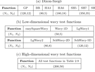
are taken for GLOBAL∗. For MLSL, N = 10 and N = 20 are taken for the first three and the last four problems of the Dixon-Szegö test bench [34], respectively.
For MATLAB’s GlobalSearch, the sample points that are evaluated before the local search is started are generated only once (whereas in SOMS, MLSL, and GLOBAL a new set of sample points is generated in each iteration). The two main algorithm parameters of GlobalSearch are the number of trial points (N1) and the number of points used in Stage 1 of the algorithm (N2). The default values for these two parameters are N1 = 1000 and N2 = 200, respectively. However, in our experiment, the maximum number of allowable
function evaluationsmf for each test functions are quite small. Thus, we used lower values for
N1andN2in order to enable several local searches before the budget of function evaluations is
exhausted. We experimented with different algorithm parameters for several combinations of (N1, N2)each with 30 trials to pick the best pair for each problem. The resulting parameters are shown in Table 2.2.
MATLAB’s MultiStart starts the local solver from a uniformly generated point (Algo-rithm 2.4), and thus there are no parameters to adjust.
For SOMS, the set of generated sample points of sizeN are not evaluated with the
expen-sive objective function. We use the computationally cheap surrogate model to predict the objective function values of these points. Thus,N can be chosen rather large. However, with
an increasing number of dimensions and increasingN, SOMS’ own computational complexity
increases, and thus a reasonable trade-off between algorithm efficiency and computational effort must be made by choosing N reasonably.
Denote by N(s), N(m), (N(GS)
1 , N
(GS)
2 ), and N(G) the parameters used in Algorithms 2.2,
2.3, 2.5, and 2.6, respectively. For example, ford= 20,mf = 2000, andN(s) =N(m) = 100d,
SOMS does 2000 computationally cheap function evaluations using the response surface. However, MLSL does these 2000 evaluation with the expensive objective function. Thus,
MLSL uses up the budget of allowable function evaluations before a local search could be started. Therefore, N(m) = 10d is a more appropriate choice. The same argument was
used when we select the parameters N for the other multistart methods. The values of the
parameters that are used for MLSL, SOMS and GlobalSearch are shown in Tables 2.1 and 2.2.
2.5
Numerical Experiments
In this section, we show the numerical results obtained for SOMS and the alternative algo-rithms. We did 30 trials with each algorithm for each test problem. For SOMS, the initial evaluation points for fitting the RBF model are generated by a symmetric Latin hypercube design (SLHD) [129]. This initial set of points is used only for fitting the RBF model and the points in this design are not used for starting the local search in Step 3a of SOMS.
2.5.1
Experimental Setup
The experiments are all run using MATLAB 7.14 (R2012a) on Intel(R) Core(TM) i7 CPU @3.40GHz 3.40 GHz. MATLAB’s fmincon is used as a local solver in all algorithms. The algorithm starts a new local optimization from the next selected point whenever the local solver has converged to a local minimum until the maximum number of function evaluations (mf) is reached. The termination tolerance of the fmincon was set to 10−8.
We chose fmincon as local solver since it is the only available local optimization method for GlobalSearch. We use the same local solver for all algorithms to facilitate a fair com-parison. We did not supply the gradient of the test function to fmincon because we treat the test functions as blackbox problems in order to determine the applicability of the var-ious methods for true blackbox problems. Thus, in each iteration of fmincon, the gradient