ENHANCEMENTS OF SPARSE CLUSTERING
WITH RESAMPLING AND CONSIDERATIONS ON
TUNING PARAMETER
by
Wenzhu Bi
B.E., Shanghai Jiao Tong University, Shanghai, China, 2000
M.S., Duquesne University, 2004
Submitted to the Graduate Faculty of
the Department of Biostatistics
Graduate School of Public Health in partial fulfillment
of the requirements for the degree of
Doctor of Philosophy
University of Pittsburgh
2012
UNIVERSITY OF PITTSBURGH
GRADUATE SCHOOL OF PUBLIC HEALTH
This dissertation was presented
by
Wenzhu Bi
It was defended on
April 9th 2012
and approved by
Lisa A. Weissfeld PhD, Professor, Department of Biostatistics
Graduate School of Public Health, University of Pittsburgh
George C. Tseng ScD, Associate Professor, Department of Biostatistics
Graduate School of Public Health, University of Pittsburgh
Yan Lin PhD, Research Assistant Professor, Department of Biostatistics
Graduate School of Public Health, University of Pittsburgh
Julie C. Price PhD, Professor, Department of Radiology
School of Medicine, University of Pittsburgh
Dissertation Director: Lisa A. Weissfeld PhD, Professor, Department of Biostatistics
Copyright c by Wenzhu Bi 2012
ENHANCEMENTS OF SPARSE CLUSTERING WITH RESAMPLING AND CONSIDERATIONS ON TUNING PARAMETER
Wenzhu Bi, PhD
University of Pittsburgh, 2012
Clustering methods are widely used to explore subgroupings in data when the true group membership is unknown. These techniques are very useful when identifying potential sub-populations of interest in the medical and public health setting. Examples of these types of subpopulations include subjects who have certain gene expression profiles related to a cancer subtype, and subjects who are in the very early, asymptomatic phase, of a chronic illness. All of these examples are of great public health relevance.
Many of the datasets of interest arise from the development of new technologies and are subject to the common problem wherep, the number of variables, is significantly larger than the sample size, n. The relatively small sample size, n, may result from the difficulties of subject recruitment and/or the financial burden of the actual data collection in fields such as imaging and genetic analysis. The earlier approaches to clustering treat all of the variables equally, which may not work well when not all of them are relevant to the subgroupings. Clustering methods with variable selection, also called sparse clustering, have been recently developed to deal with this problem. We propose a method to add resampling onto sparse clustering to improve upon the current clustering methodology. The addition of resampling methods to sparse clustering results in variable selection that is more accurate. The method is also used to assign an“observed proportion of cluster membership” to each observation, providing a new metric by which to measure membership certainty. The performance of the method is studied via simulation and illustrated in the motivating data example.
an adjusted Bayesian Information Criterion (BIC). Variable selection in sparse clustering is realized by applying Lasso or related penalties and the tuning parameter for these penalties has to be determined beforehand. The gap statistic, a distance-based approach, is used to choose the tuning parameter through permutation and it may behave poorly at times. The proposed BIC approach is an alternative developed under the more sophisticated model-based likelihood framework. Its performance is evaluated with simulations.
TABLE OF CONTENTS
PREFACE . . . x
1.0 INTRODUCTION . . . 1
2.0 SPARSE CLUSTERING WITH RESAMPLING . . . 6
2.1 Introduction . . . 6
2.2 Methods. . . 8
2.2.1 K-means Clustering . . . 8
2.2.2 Sparse K-means Clustering . . . 10
2.2.3 The Proposed Method. . . 11
2.3 Simulation Study . . . 13
2.3.1 Simulation 1 . . . 13
2.3.2 Simulation 2 . . . 15
2.3.3 Methods Comparison . . . 17
2.4 Application in Neuroimaging Data . . . 21
2.5 Conclusions and Discussion . . . 25
3.0 TUNING PARAMETER CHOICE FOR SPARSE K-MEANS CLUS-TERING . . . 28
3.1 Introduction . . . 28
3.2 Gap Statistic for Tuning Parameter Choice . . . 30
3.3 Tuning Parameter Choice in Penalized Model-based Clustering . . . 31
3.3.1 Model-based Clustering . . . 31
3.3.2 Penalized Model-based Clustering . . . 32
3.4 Problematic Results using Gap Statistic . . . 34
3.5 The Proposed Method: Using an Adjusted BIC for Tuning Parameter Choice in Sparse K-means Clustering . . . 38
3.5.1 The Proposed Method. . . 38
3.5.2 A Simple Example . . . 39
3.5.3 Simulation Results . . . 41
3.6 Conclusions and discussions . . . 41
4.0 OTHER WORK . . . 43
LIST OF TABLES
1 Tight cluster results in Simulation 1 . . . 15
2 Tight cluster results in Simulation 2 . . . 17
3 Cluster results in Simulation 3 . . . 19
4 Variable selection results in Simulation 3 . . . 20
5 Tuning parameter choice for a problematic scenario withp= 500 . . . 34
6 Tuning parameter choice for another problematic scenario with p= 1000 . . . 35
7 The results using the adjusted BIC for tuning parameter choice in an imaging dataset . . . 40
LIST OF FIGURES
1 The number of journal articles with k-means clustering. . . 3 2 Group average within each variable in an example of the simulated dataset. . 13 3 Voxel/Variable weights in the brain imaging example . . . 24 4 Variable weights in a problematic scenario with the gap statistics . . . 36
PREFACE
I thank my primary advisor Dr. Lisa A. Weissfeld for her vision, guidance, and help. She introduced me to the field of brain imaging research. With her encouragement and support, I have gained invaluable training and experiences. She supported me to join the graduate training program at the Center for the Neural Basis of Cognition to gain in-depth training in neuroscience. She encouraged me to take courses and to attend imaging workshops through-out the country to build up the skill set. During the dissertation work, she allowed me to pursue topics of my own interest and shared her wisdom along the way.
I thank my committee member and also co-advisor, Dr. George C. Tseng, for his in-valuable advice. He inspired my interest and confidence in clustering through classroom teaching and individual research meetings. He provided critical feedback for many aspects of the work. His research group provided me crucial support for using the Linux computing server. I also thank my committee member Dr. Yan Lin for her insightful suggestions to improve the quality of this dissertation.
Special gratitude goes to my imaging mentor Dr. Julie C. Price. She gave me the oppor-tunity to work on the radiotracer Pittsburgh compound-B, a major scientific breakthrough in Alzheimer’s disease research. Like Dr. Weissfeld, Dr. Price has been very supportive in every single step of my career development. I am thankful for her encouragement, support, and guidance.
Hearty thanks goes to my classmates, colleagues and friends in Pittsburgh for their help and support. I sincerely thank my closest friends and colleagues Dr. Bedda L. Rosario and Rhaven L. Coleman for their encouragements and support. At last, I thank my husband Darrick W. Mowrey and our family for their love, support and encouragements.
1.0 INTRODUCTION
Large datasets have been easily generated by the advancement in computation in the last twenty years. They exist in the fields of genetics, imaging, chemometrics and many others. Many of these datasets have the property of “high-dimension, low sample size” (p n), which means that the number of variables,p, is much larger than the number of observations, n. For example in DNA microarray data, the expression levels for tens of thousands genes can be observed while there are usually dozens or hundreds of subjects in a study. In neuroimaging, there could be hundreds of thousands of voxels per brain scan with only a few dozen subjects in a study. The challenge is to extract useful information from this abundance of data and statistical learning methods have evolved to address these issues.
Statistical learning can be roughly categorized into supervised learning and unsupervised learning depending on whether the true group membership is known or not. If the true membership is known, it can serve as a guide for the construction of the statistical learning method, hence it is named supervised learning. Classification is a classic example. When the true group membership is unknown, we lose this crucial information for guidance; hence it is called unsupervised learning. Clustering is a classic example of unsupervised learning and it is also the focus of this dissertation work.
Clustering analysis usually aims to group a collection of objects into clusters “such that those within each cluster are more closely related to one another than objects assigned to different clusters” as defined by Hastie, Tibshirani and Friedman[15]. Correspondingly, the algorithms try to maximize the between-cluster difference while minimizing the within-cluster difference. The difference is called dissimilarity, which can be Euclidean distance (i.e., squared difference), Manhattan distance (i.e., absolute difference) or other metrics depending on the problem. Euclidean distance is most commonly used for the dissimilarity measure.
Typical clustering methods include k-means clustering, k-medoids clustering, hierarchical clustering and model-based clustering.
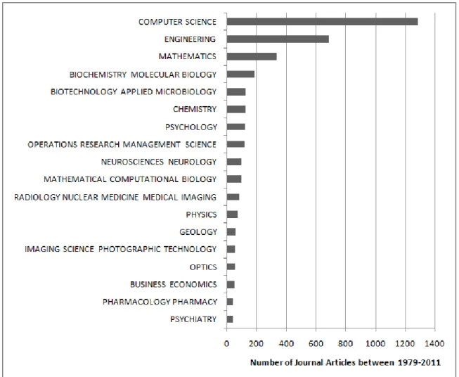
K-means clustering is one of the most popular clustering methods[15]. It and its variants have been widely applied in various fields such as computer science, engineering, business, economics, biology, chemistry, psychology, neurology, medical imaging, pharmacology and psychiatry as shown in Figure ??. It can be traced back to work done by Lloyd in 1957[20], by Forgy in 1965[6], by MacQueen in 1967[21] and by Hartigan and Wong in 1979[13]. The algorithm was significantly improved by Hartigan and Wong(1979)[13]. K-medoids clustering is very similar to k-means. The only difference is that the cluster center is the object closest to the cluster mean while in k-means the cluster center is the cluster mean; in other words, the cluster centers are medoids rather than centroids. K-medoids clustering is more robust to outliers for this reason[18]. K-means and k-medoids require the user to specify the number of clusters while hierarchical clustering does not require so. Hierarchical clustering[16] provides a dendrogram as the results, which shows a summary of the data. The dendrogram can be built with either an agglomerative(bottom-up) or a divisive(top-down) approach. The distance between clusters can be defined in various ways such as defined by the closest pair of objects between two clusters, or the furtherest pair, or as the average of all the pairs.
K-means, k-medoids and hierarchical clustering methods are considered to be heuristic distance-based clustering methods. Parametric models have also been developed for cluster-ing, resulting in model-based clustering techniques. The advantage of model-based clustering is the ability to draw statistical inference. A very successful model is the finite mixture model such as work done by McLachlan and Basford in 1988[25], Banfield and Raftery in 1993[1], and Fraley and Raftery in 1998[7] and 2002[8]. The last two papers discussed different co-variance structures. The estimation was realized by EM algorithm and the model selection by Bayesian Information Criterion (BIC).
For a dataset, Xn×p, with n observations and p variables per observation, earlier
ap-proaches to clustering tend to treat all of the variables equally. It may not work well when not all of them are relevant to the subgroupings, which is especially true in the case of the “high-dimension, low sample size” (p n) problem. Clustering methods with variable se-lection, also called sparse clustering methods, have been recently developed to deal with this
Figure 1: The number of journal articles between 1979 and 2010 with k-means clustering categorized by subject area. Shown above is a sample of the subject areas. Citation data is obtained from web of knowledge (http://wokinfo.com/).
problem. Many of the sparse clustering methods make use of anL1/Lasso penalty or related penalties to realize variable selection. A general framework for clustering was proposed by Witten and Tibshirani in 2010 [35]. It applied both an L1 and anL2 restraint to realize vari-able selection. It was demonstrated with sparse k-means and sparse hierarchical clustering. These penalties were also applied to the model-based clustering framework. Pan and Shen in 2007[27] proposed a penalized model-based clustering method, in which BIC was used for model selection. The penalized mixture model assumes independence between variables and the same diagonal covariance matrix across clusters. The development of sparse clustering analysis is moving clustering into a new era and allowing us to sift the data more closely than we have ever been able to.
In this dissertation work we develop two new methods under the scope of sparse clus-tering. The first method is motivated by the problem of small sample size. For example, a neuroimaging dataset with a few dozens of subjects is common due to the challenges in subject recruitment and the cost of scans. Clustering of such data is important in exploring the patterns associated with different underlying biological characteristics and in searching for a disease detection threshold. Often times, due to the limitations of the sample size, one would consider issues such as “How representative is the sample of the population?” or “If we were going to construct clusters, how much confidence can we have in the clustering results?” We propose a method to add resampling onto sparse clustering to address these concerns. This method will alleviate the effects of noise and outliers on the variable selection and clustering results and generate confidence levels for the clustering results.
The second method is about the choice of the tuning parameter. The results of theLasso -related penalties depend on the tuning/penalization parameter choice. The magnitude of the tuning parameter relates to the number of variables selected for clustering. The choice of the tuning parameter has been studied in regression and classification with cross-validation being the main approach. This method can not be easily applied to clustering methods due to the lack of information on the true group membership. Pan and Shen in 2007[27] used a modified BIC to determine both the number of clusters and the tuning parameter. Witten and Tibshirani in 2010[35] proposed using the gap statistic. Yet both of these methods rely on the correct specification of the tuning parameter pool. We have observed that given
a suboptimal pool the gap statistic method could choose a tuning parameter which yields poor performance when clustering, i.e. a high Classification Error Rate (CER). When this happens it usually chooses a tuning parameter that is either too small or too large, hence too few, or too many, variables are chosen for clustering. This is more likely to occur when the overlap between the clusters is more substantial. In this work, we would like to draw attention to this phenomenon and also to propose using the BIC for the choice of the tuning parameter for the sparse k-means method proposed by Witten and Tibshirani in 2010 [35].
The two methods will be described separately in the next two chapters. Chapter 2 includes an introduction to the background, the methods section, simulation study results and an application to the motivating imaging dataset. In chapter 3, we give an introduction to the background, the existing methods, scenarios where gap statistic has failed, and the proposed method to address the issue. The method is demonstrated via a real example and simulation studies. The last chapter summarizes the conclusions of this work.
2.0 SPARSE CLUSTERING WITH RESAMPLING
2.1 INTRODUCTION
Large datasets have become commonplace due to the advancement in computation and other technologies in the last twenty years. They exist in the fields of genetics, imaging, chemomet-rics and many others. Many of these datasets have the property of “high-dimension, small sample size” (p n), where the number of variables, p, is much larger than the number of observations, n. For example in DNA microarray data, the expression levels for tens of thousands of genes can be observed while there are usually dozens or hundreds of subjects in a study. In neuroimaging, there could be hundreds of thousands of voxels per brain scan with only a few dozen subjects in a study. The challenge is to extract useful information from this abundance of data and statistical learning methods, including clustering, have evolved to address these issues.
Clustering aims to group a collection of observations into clusters “such that those within each cluster are more closely related to one another than objects assigned to different clus-ters” as defined by Hastie, Tibshirani and Friedman [15]. It can be used to discover and identify biologically distinct subgroups from ann×pdataset without knowledge of the true group membership and plays an important role in the earlier stage of scientific studies when no definite group membership can be assigned to the observations. Clustering can also be used to establish rules for predicting memberships for additional observations, where par-simonious rules are desirable for prediction accuracy. As the definition implies, clustering algorithms are designed to maximize the between-cluster difference while minimizing the within-cluster difference. This difference, referred to as dissimilarity, can be measured using Euclidean distance (i.e., squared difference), Manhattan distance (i.e.,absolute
dif-ference) or other metrics depending on the problem. Typical clustering methods include k-means clustering, k-medoids clustering, hierarchical clustering and model-based cluster-ing, with k-means clustering being one of the most popular clustering methods. It and its variants have been widely applied in various fields such as computer science, engineering, business, economics, biology, chemistry, psychology, neurology, medical imaging, pharmacol-ogy and psychiatry. It can be traced back to work done by Lloyd in 1957 [20], by Forgy in 1965 [6], by MacQueen in 1967 [21] and by Hartigan and Wong in 1979 [13], with Hartigan and Wong significantly improving the algorithm for identifying clusters. Resampling was used as an approach in “tight clustering” by Tseng and Wong in 2005 [34] to deal with noisy observations and to construct reliable tight clusters. Compared to regular clustering analysis which tends to group all n observations into clusters, tight clustering will leave out those scattered noisy samples to construct stable and reliable clusters. This was motivated by microarray studies where the goal was to find robust patterns reflecting the underlying biological process.
For a dataset, Xn×p, with n observations and p variables per observation, earlier
ap-proaches to clustering tend to treat all of the variables equally. This may not work well when not all of the variables are equally relevant to the subgroupings, which is especially true in the case of the “high-dimension, small sample size” (p n) problem. Clustering methods with variable selection, also called sparse clustering methods, have been recently developed to deal with this problem. Many of the sparse clustering methods make use of an L1/Lasso penalty or related penalties to realize variable selection with Witten and Tibshi-rani in 2010 [35] applying both an L1 and an L2 restraint to implement variable selection. These penalties were also applied to the model-based clustering framework. Pan and Shen in 2007 [27] proposed a penalized model-based clustering method, in which BIC was used for model selection. The penalized mixture model assumes independence between variables and the same diagonal covariance matrix across clusters. Sparse clustering methods choose the variables that more accurately reflect the variability in the original dataset while diminishing or eliminating the effects of less relevant variables on the clustering. The resulting clustering rules are more parsimonious, easier to interpret, and could yield a more desirable prediction accuracy. This is true when p < nbut it is more evident when pn.
In this work our goal is to deal with the problem of small sample size. It is motivated by an example arising from the identification of potentially “positive” subjects for amyloid deposition, a protein that is believed to be key in identifying subjects that will go on to develop Alzheimer’s disease. The goal is to identify these subjects before they develop any of the symptoms of the disease with the hope of potential treatments to prevent the onset of symptoms. Clustering of such data is important in exploring the patterns associated with different underlying biological characteristics and in searching for a disease detection threshold. We propose a method to add resampling onto sparse clustering in order to provide a “certainty measure” for group membership.
This method combines sparse k-means and resampling, so that one can achieve variable selection and tight clusters at the same time. By resampling we will be able to more reli-ably select the variables and to compute a confidence level for the clustering results. This confidence level will be described in more detail in later sections. With this metric we could also construct tight clusters while leaving the outlier or noisy observations outside of these reliable clusters. We could also potentially identify the degree of the overlap between clus-ters. The methodology is described in Section 2. Simulation studies are shown in Section 3 to demonstrate how the proposed method works and to compare its performance to those of k-means and sparse k-means. The application of the proposed method in a neuroimaging dataset is shown in Section 4. In Section 5 we discuss the strength and limitations of the method and some problems we encountered during this work.
2.2 METHODS
2.2.1 K-means Clustering
LetXij denote a dataset of sizen byp, wherenis the number of observations in the dataset,
p is the number of variables observed for each observation, i = 1, ..., n and j = 1, ..., p. K-means clustering aims to group n observations into K clusters such that the within cluster dissimilarity across all clusters is minimized. The squared Euclidean distance is used as the
dissimilarity measure. The algorithm aims to minimize the within-cluster sum of squares (WCSS), so the target function is defined as
minimizeC1,C2,...CK ( K X k=1 1 nk X i∈Ck p X j=1 (xij −µkj)2 ) , (2.1)
where the clusters are denoted as C1, C2, . . . , CK, with nk being the number of observations
in each cluster. µk. is the cluster center for the kth cluster, also called centroid, which is
computed as the arithmetic average of all the observations in that cluster. µkj is the average
on the jth dimension.
The most widely used algorithm for k-means is the one that was developed by Hartigan and Wong in 1979. The main idea is an iterative algorithm with the following steps:
1. Set random cluster centers.
2. Assign each observation to the appropriate cluster based on the squared Euclidean dis-tance from each cluster center.
3. Given the cluster membership, compute the new cluster centers.
4. Iterate between Step 2 and Step 3 until the cluster membership does not change any more.
It is best to use more than one set of random cluster centers in Step 1 because of the potential problem of local maxima. We assume that the number of clusters, K, can be pre-specified. If the number of clusters is in question, it can be potentially determined by gap statistic [33] or many other methods.
Equation (2.1) is mathematically equivalent to maximizing the between-cluster sum of squares (BCSS), that is,
maximizeC1,C2,...CK ( 1 n n X i=1 (xi−µ..) 2 − K X k=1 1 nk X i∈Ck (xi−µk.) 2 ) , (2.2)
whereµ..is the cluster center ifK = 1, which is the average of allnobservations. The average
distance of all observations from this single cluster center is n1Pn
i=1(xi−µ..)
2
, which is also called total sum of squares (TSS).
If we calculate the values of TSS and BCSS on each dimension first and then sum across the variables, Equation (2.2) becomes:
maximizeC1,C2,...CK p X j=1 ( 1 n n X i=1 (xij −µ.j) 2 − K X k=1 1 nk X i∈Ck (xij−µkj) 2 ) , (2.3)
where µ.j is the value of µ.. on thejth dimension. Equations (2.2) and (2.3) form the basis
for understanding the equations for sparse k-means.
2.2.2 Sparse K-means Clustering
Sparse k-means clustering was proposed by Witten and Tibshirani in 2010 [35]. This ap-proach minimizes the target function of the weighted BCSS with the variable weights subject to an L1/Lasso condition and an L2 condition. An EM algorithm is used for obtaining the solutions and it alternates between the weighted k-means and convex optimization with a soft-thresholding operator until convergence is reached. The results are the variable weights and cluster membership. The variable weights are assigned to the variables so that greater weight is given to the variables of greatest importance. Note that some variables have zero weights meaning that they are not used in the final clustering results. The sparse k-means clustering criteria is parsimonious for prediction and most useful whenpnbut also works well whenp < n.
Instead of treating all variables equally as in k-means clustering, sparse k-means clus-tering will assign weights wj to variables. The target function and its constraints are the
following: maximizeC1,C2,...CK,w ( p X j=1 wj 1 n n X i=1 (xij−µ.j)2− K X k=1 1 nk X i∈Ck (xij −µkj)2 !) (2.4) subject to ∀j, wj ≥0,kwk2 ≤1,kwk1 ≤s, where
• w is a vector with length p. Each element wj serves as a weight for each variable. All
weights are nonnegative values.
• kwk1 ≤s is the L1/Lasso condition, meaning that the sum of the absolute values of the weights is less than s, the tuning parameter.
• kwk2 ≤1 is the L2 condition, meaning that the square root of the summation of the squared values of the weights is less than or equal to 1.
To solve for the weights and the cluster membership, Witten and Tibshirani [35] proposed the following iterative method:
1. Assume that all variables have the same weight √1
p.
2. Given the weights, find the cluster membership using the k-means algorithm. K-means is applied to the data after the variables are scaled appropriately by the squared root of the corresponding weights, which can be regarded as weighted k-means.
3. Given the cluster membership, solving for the weights can be regarded as a convex problem. To optimize the convex problem, one can apply soft-thresholding as described in Witten and Tibshirani [35].
4. Iterate between Step 2 and Step 3 until the weights converge.
The results of the sparse k-means clustering are the weights for all of the variables and the cluster membership of the individual observations. The variable weights were divided by the tuning parameter for standardization in this work. These standardized variable weights can be used for comparison between clustering results with different tuning parameters.
2.2.3 The Proposed Method
For the datasets with the property of “high-dimension, small sample size” (p n), we propose this method that combines sparse k-means and resampling, so that one can select the variables important to clustering and construct tight clusters at the same time. At each resampling of the dataset, the variable weights and the cluster membership are obtained. These results are then summarized across all of the resampling runs.
The main idea of the proposed method is to resample the original dataset Xn×p for
a number of times, B, and to apply sparse k-means clustering to each sample. For each resampling run, we randomly sample 70% of the observations without replacement and predict the cluster membership for the remaining 30% of the observations based on the sample results, similar as the method proposed in [34].
The algorithm is described as follows:
1. Randomly choose a sample with 70% of observations (or rows) without replacement from the original dataset Xn×p. Let us denote this subset of the dataset X0.
2. Apply sparse k-means on X0. The number of clusters, K, should be pre-specified and remains the same for all resampling runs.
3. Apply the clustering criterion obtained from Step (2) and predict the cluster membership for the remaining 30% of the original dataset X.
4. Repeat steps (1)-(3) for a number ofB times. Each variable is assigned a weight for each of the B times and the cluster membership for all n observations are obtained B times. 5. Select variables and construct tight clusters with information from Step (4). Since the tuning parameters may be different across the resampling runs, the variable weights were divided by the tuning parameter in that resampling run for standardization. The final weight for each variable can be simply computed as the average across its standardized weights from all B random samples.
Theconf idence levelis defined to be the proportion of times for an observation to appear in a cluster. For example, if the observation xi appears in the cluster Ck for a number
of bk times out of the B resampling runs, the confidence levelCLik is computed asbk/B
and PK
k=1CLik = 1. Confidence levels for all observations are computed.
To construct tight clusters, a threshold for the confidence level, denoted as t, should be specified. For example,t = 95% ort= 90%. The observations with a confidence level≥t will be included in the tight clusters and the remaining observations will be left outside of the tight clusters. If the true underlying groups overlap with each other, the proposed method can potentially identify the degree of this overlap through the construction of the tight clusters.
2.3 SIMULATION STUDY
2.3.1 Simulation 1
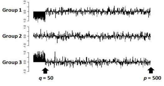
We simulated data as described in Witten and Tibshirani (2010) [35]. The simulated dataset, Xn×p, hadn = 60 observations andpvariables per observation. The sixty observations form
three groups with twenty observations per group Gk, where k = 1,2, and 3. These groups
were generated to have different means across the three groups for the first q= 50 variables but not for the remainingp-q variables. That is:
• For j = 1,2,· · · , q, Xi ∈ Gk ⇔ Xij ∼ N(µk,1), where µ1 = −µ, µ2 = 0, µ3 = µ. For the first q= 50 variables, the data were generated from three normal distributions with different mean values but the same variance 1.
• For j = q+ 1,· · · , p, Xij ∼ N(0,1). For the remaining p-q variables, the data were
generated from the same standard normal distribution.
Figure 2: Group average within each variable in an example of the simulated dataset.
We chose a scenario with p= 500 andµ= 0.7 to demonstrate how the proposed method works. We generated 250 simulated datasets and resampled each datasetB = 20 times.
The variable weight for the proposed method was computed as the average across the B = 20 resampling runs. The variable weights were then summarized over the 250 simulated
datasets. On average the first 50 variables have weights in the range of 0.012-0.016 (stan-dard error: 0.0006-0.0018) and the remaining 450 variables have weights in 0.0005-0.0009 (standard error: 3.3×10⁻⁵-0.0002). The weights for the first 50 variables were 13 to 32 times greater than those associated with the remaining uninformative 450 variables, indicating that the proposed method was able to identify the variables of greatest importance in determining cluster membership.
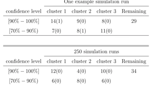
Table 1 shows the results for the tight clusters. The results for one example simulated dataset are presented in the top part of the table. The dataset was resampled 20 times. The confidence level is the observed proportion of times that an observation falls in a given cluster over the 20 resampling runs. For example, 100% indicates that 20 out of 20 times the observation was chosen to be in a specified cluster, 90% indicates that 18 out of 20 times the observation appeared in a cluster and 70% indicates that 14 out of 20 times. The confidence levels were computed for each observation for all of the clusters. With a confidence level ≥ 90%, there were 14 observations in cluster 1, 9 observations in cluster 2, and 8 observations in cluster 3 with one observation missclassified into cluster 1. The remaining 29 observations were left outside of these tight clusters. The three groups in the simulated dataset were overlapping because of µ = 0.7. These results were consistent with this overlap. If the groups were well separated, there should be fewer observations left outside of the tight clusters. At the confidence level ≥ 70% and < 90%, there were 7 addtional observations classified into cluster 1, 8 additional observations in cluster 2 and 11 additional observations in cluster 3 including one observation missclassified into cluster 2. If we relaxed the confidence level threhold to be ≥ 70% for the tight clusters, there were 21 observations in cluster 1, 17 observations in cluster 2, and 19 observations in cluster 3. Among these observations one observation in cluster 1 and another one in cluster 2 were misclassified. The remaining 3 observations were not included in any of these tight clusters.
The results for 250 simulated datasets are shown in the bottom part of Table 1. With a confidence level ≥90%, on average there were 12 observations in cluster 1, 4 observations in cluster 2, and 10 observations in cluster 3. The remaining 34 observations were left outside of these tight clusters. When the confidence level threshold was relaxed to be ≥ 70%, on
Table 1: Tight clusters for the scenario withµ= 0.7 andp= 500. Top Panel: The number of observations in a cluster for one example simulated dataset. Bottom Panel: Average number of observations in tight clusters across 250 simulated datasets. Each dataset was resampled B = 20 times. The numbers of misclassified observations are given in the parentheses.
One example simulation run
confidence level cluster 1 cluster 2 cluster 3 Remaining
[90%−100%] 14(1) 9(0) 8(0) 29
[70%−90%) 7(0) 8(1) 11(0)
250 simulation runs
confidence level cluster 1 cluster 2 cluster 3 Remaining
[90%−100%] 12(0) 4(0) 10(0) 34
[70%−90%) 6(0) 8(0) 6(0)
average there were 6 additional observations classified into cluster 1, 8 additional observations in cluster 2, and 6 additional observations in cluster 3. The remaining 14 observations were left outside of the tight clusters. These results were also consistent with the group overlap in the simulated datasets.
Simulation 1 demonstrated how the proposed method achieves variable selection, com-putes the clustering confidence level, and constructs tight clusters. It was able to identify the variables which were more important to clustering and to indicate the overlap in the simulated datasets.
2.3.2 Simulation 2
This simulation is similar to Simulation 1 except that more scenarios are considered. There was one scenario with p = 500 and µ = 0.7 in Simulation 1; In this simulation, p = 50, 200, 500 & 1000 and µ= 0.6, 0.7, 0.8, 0.9 & 1.0, so that there were a total of 20 scenarios.
Out of the p variables, the three groups were different in the first q= 50 variables while not distinguishable in the remaining p-q variables. The first q = 50 variables were different in a way that the first group was sampled from the normal distribution N(−µ,1), the second group from N(0,1), and the third group from N(µ,1). The remaining p-q variables were sampled from the same standard normal distribution. The value of µis an indicator of the overlap between the groups in theq variables. The overlap is most substantial whenµ= 0.6 and decreases as µ gets bigger. The groups were best separated when µ= 1.0. There were 25 simulated datasets for each scenario and each dataset was resampled B = 100 times.
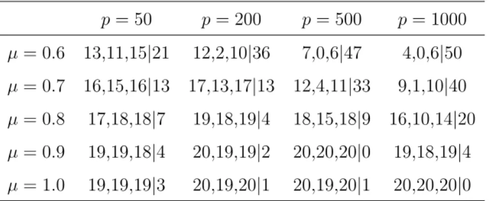
Table 2 presents the simulation results for 20 scenarios where p = 50, 200, 500 & 1000 and µ= 0.6, 0.7, 0.8, 0.9 & 1.0. Tight clusters were constructed to include the observations with a confidence level ≥90%, which indicates that the observation appeared in the cluster at least 90 times out of B = 100 times. The average values were computed across the 25 simulated datasets for the number of correctly classif ied observations in each cluster and the number of remaining observations. They are listed as (cluster 1, cluster 2, cluster 3 | remaining) in Table 2. For example, for the scenario with p= 500 and µ= 0.7, on average there were 12 observations in cluster 1, 4 observations in cluster 2 and 11 in cluster 3 and the number of remaining observations was 33.
We noticed that the method was able to identify the degree of the overlap between the groups indicating by the increasing number of remaining observations as µ gets smaller. When µ= 1.0, the groups were best separated and the method was able to correctly place at least 19 observations out of 20 observations in each tight cluster with a confidence level ≥ 90%. As µ decreases, there were fewer observations included in the tight clusters. The smallest tight cluster was the middle group since it overlapped with the other two groups on both sides. As the number of variables, p, gets larger and µ is closer to 0, the method struggles to identify the clusters, while it performs well in settings where there is some separation.
Table 2: The average number of correctly classified observations in each cluster and the average number of remaining observations (cluster 1, cluster 2, cluster 3 | remaining) with a confidence level ≥ 90%. The average was computed over 25 simulated datasets in each scenario. Each dataset was resampled B = 100 times. The number of the truly different variables was q= 50. p= 50 p= 200 p= 500 p= 1000 µ= 0.6 13,11,15|21 12,2,10|36 7,0,6|47 4,0,6|50 µ= 0.7 16,15,16|13 17,13,17|13 12,4,11|33 9,1,10|40 µ= 0.8 17,18,18|7 19,18,19|4 18,15,18|9 16,10,14|20 µ= 0.9 19,19,18|4 20,19,19|2 20,20,20|0 19,18,19|4 µ= 1.0 19,19,19|3 20,19,20|1 20,19,20|1 20,20,20|0 2.3.3 Methods Comparison
The goal of this simulation study was to compare three clustering methods: k-means, sparse k-means and the proposed method “sparse k-means and resampling”. We use all of the datasets generated in Simulation 2 for all 20 scenarios. K-means, sparse k-means and the proposed method were applied to these datasets with K = 3. The clustering results are summarized in Tables 3 and 4. For sparse k-means and the proposed method, the tuning parameter pool was the same in each scenario, which is a vector of 15 values within the range (3.5, 0.7×√p).
The performance of clustering was measured by the classif ication error rate or CER [35]. In this simulation study, it is a measure of disagreement between the true group mem-bership and the cluster memmem-bership. The CER value can range from 0 to 1. A classification error rate with value 0 indicates a perfect agreement, or no disagreement, between the group membership and the cluster membership. The bigger the CER value, the less accurate the clustering recovered the true group membership.
Table 3lists the average classification error rate (CER) values along with their standard errors across the 25 simulated datasets in each scenario. The results for each of the three methods were given. For the proposed method, this CER value was calculated for the subset of those observations in the tight clusters with confidence level ≥90%. We used the classification error rate for the comparison of these methods so that others can relate our results with those in Witten and Tibshirani (2010) [35], but we were aware of the limitations of this measure. In the simulation study the true group membership were assigned when the data were generated. If there was overlap between groups, the observations mixed in the overlap were given different group membership; When clustering was applied, it was blind to the true group memberhsip and could hardly disentangle this mixed overlap back into the correct clusters, so it was almost impossible to achieve clustering results which perfectly agrees to the true group memberhsip. With the tight clusters constructed by the proposed method, we were able to achieve smaller classification error rates because of the fact that it was calculated for the observations in the tight clusters only, which were usually not part of the overlap.
When p = q = 50 in Table 3, since all of the 50 variables were different and they were different in the same way between the groups, k-means achieved smaller CER values than sparse k-means. Sparse k-means might have tried to assign different weights to the variables, which could be the reason for the smaller CER values. It is worthwhile to point out, although it is not the case here, that if the group difference varies across the variables, sparse k-means may be a better method than k-means. When q = 50 andp= 200,500 and 1000, there were only a subset of q variables that were different across groups. The CER values for sparse k-means were smaller than those from k-means. This was because under these scenarios while k-means treated all of the variables the same way, sparse k-means was able to discover the variables important to clustering and to leave out the irrelevant variables. For all twenty scenarios the proposed method achieved even smaller CER values than the other two methods, this was because the CER value was computed for the subset of those observations in the tight clusters. These very small CER values (range: 0.000-0.032) indicates that the observations in the tight clusters were recovered from the corresponding true groups with a very high accuracy.
Table 3: The average classification error rate (standard error) over 25 simulated datasets for each scenario. For our proposed method “sparse k-means and resampling”, each dataset was resampled B = 100 times and the classification error rates were calculated for those observations with a confidence level ≥90%.
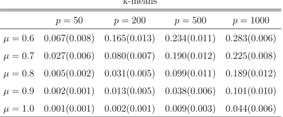
k-means p= 50 p= 200 p= 500 p= 1000 µ= 0.6 0.067(0.008) 0.165(0.013) 0.234(0.011) 0.283(0.006) µ= 0.7 0.027(0.006) 0.080(0.007) 0.190(0.012) 0.225(0.008) µ= 0.8 0.005(0.002) 0.031(0.005) 0.099(0.011) 0.189(0.012) µ= 0.9 0.002(0.001) 0.013(0.005) 0.038(0.006) 0.101(0.010) µ= 1.0 0.001(0.001) 0.002(0.001) 0.009(0.003) 0.044(0.006) sparse k-means p= 50 p= 200 p= 500 p= 1000 µ= 0.6 0.133(0.011) 0.137(0.014) 0.197(0.013) 0.252(0.011) µ= 0.7 0.067(0.008) 0.056(0.006) 0.087(0.016) 0.136(0.017) µ= 0.8 0.040(0.005) 0.017(0,005) 0.025(0.006) 0.045(0.011) µ= 0.9 0.015(0.004) 0.009(0.004) 0.006(0.002) 0.008(0.002) µ= 1.0 0.008(0.003) 0.001(0.001) 0.001(0.001) 0.002(0.001)
sparse k-means and resampling
p= 50 p= 200 p= 500 p= 1000 µ= 0.6 0.032(0.007) 0.016(0.006) 0.008(0.005) 0.004(0.004) µ= 0.7 0.009(0.003) 0.006(0.002) 0.003(0.002) 0.015(0.007) µ= 0.8 0.003(0.002) 0.000(0.000) 0.001(0.001) 0.002(0.001) µ= 0.9 0.001(0.001) 0.003(0.002) 0.002(0.001) 0.002(0.001) µ= 1.0 0.000(0.000) 0.000(0.000) 0.000(0.000) 0.000(0.000)
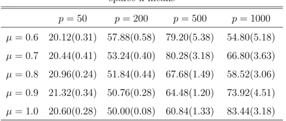
Table 4: The average number (standard error) of variables with weights>1/p. The average was computed over 25 simulated datasets for each scenario. For our proposed method “sparse k-means and resampling”, each dataset was resampled B = 100 times. The number of variables truly different between groups was q= 50.
sparse k-means p= 50 p= 200 p= 500 p= 1000 µ= 0.6 20.12(0.31) 57.88(0.58) 79.20(5.38) 54.80(5.18) µ= 0.7 20.44(0.41) 53.24(0.40) 80.28(3.18) 66.80(3.63) µ= 0.8 20.96(0.24) 51.84(0.44) 67.68(1.49) 58.52(3.06) µ= 0.9 21.32(0.34) 50.76(0.28) 64.48(1.20) 73.92(4.51) µ= 1.0 20.60(0.28) 50.00(0.08) 60.84(1.33) 83.44(3.18)
sparse k-means and resampling
p= 50 p= 200 p= 500 p= 1000 µ= 0.6 20.76(0.40) 50.96(0.46) 63.92(2.13) 102.00(4.25) µ= 0.7 21.20(0.42) 52.44(0.42) 59.00(1.12) 62.72(1.16) µ= 0.8 20.76(0.30) 51.48(0.37) 55.52(0.73) 56.80(0.65) µ= 0.9 21.04(0.35) 50.64(0.25) 55.80(0.51) 55.60(0.53) µ= 1.0 20.92(0.30) 50.04(0.09) 54.84(0.42) 51.76(0.35)
Table 4 lists the average number (and its standard error) of variables with the final standardized weights > 1/p. It was summarized from results with sparse k-means and the proposed method “sparse k-means and resampling”. Recall from the methods section, for sparse k-means the final variable weight was the standardized weight, which was the original variable weight divided by tuning parameter; for the proposed method the final variable weight was the average standardized weight over B = 100 resampling runs. Because of the standardization, the final weights were comparable between clustering results with different tuning parameters. If all of the variables were equally important to the clustering, each variable would have been assigned the same weight 1/p. We counted the number of the variables with final weights >1/p, which were also the variables that affect clustering more than they would have if all of the p variables were treated equally.
Recall that the number of variables that were truly different between groups was q = 50 while the number of variables p= 50, 200, 500, and 1000. When p= 50, both of the sparse k-means and the proposed method assigned weights>1/pto about 20 variables and weights ≤ 1/p to the remaining variables. These methods were not a good choice here since all of theq = 50 variables were generated to be similarly different between groups. Whenp= 200, 500, and 100, the proposed method were able to more closely identify important variables in that the number of variables with weights > 1/p was closer to the number q = 50 than that of sparse k-means in most of scenarios. An acceptable exception was the scenario with µ = 0.6 and p= 1000 because the aforementioned problem with this scenario. Overall the proposed method was able to identify the variables with greatest importance to clustering and its performance was better than that of sparse k-means in scenarios where pgets larger.
2.4 APPLICATION IN NEUROIMAGING DATA
We apply the proposed method to a brain imaging dataset. At first we will describe the background for this application. According to the Alzheimer’s Association 2011 Alzheimer’s Disease Facts and Figures, the neurological degenerative disease, Alzheimer’s Disease (AD), counts for about 60-80% cases of dementia. It is estimated that “5.4 million Americans
are living with” the disease. It is “the 6th leading cause of death” in the country and “the only cause of death among the top 10 that cannot be prevented, cured or even slowed” (http://www.alz.org/). Amyloid-β(Aβ) plaque deposition is a hallmark for AD neuropathol-ogy. Studies have shown that the amyloid deposition could have started more than a decade before the onset of any memory symptoms. It is of great interest to detect those people who are at risk of developing AD. Early detection of these individuals may allow a slowing or stoppage of the progress of the disease long before its onset.
The definitive diagnosis of AD can only be given by pathological tests after the patient has deceased; the ante-mortem diagnosis is “Probable AD”. The development of [11C] Pittsburgh compound-B (PiB) PET imaging agent allowed imaging of Amyloid-β(Aβ) deposition in living humans in 2003 [19,22]. PiB has been widely studied by many institutions and large-scale studies are under way in the United States, Japan and Australia. It can potentially serve as an in-vivo test to monitor the progress of amyloid deposition and a surrogate measure for treatment effectiveness. Developing thresholds for detecting those cognitively normal people who are at risk of developing AD based on the data from the PiB PET scans has been an ongoing research focus among the Pittsburgh Amyloid Imaging group, whom we collaborate closely with.
Establishing the AD early detection diagnostic criteria is facing crucial challenges due to the lack of information for a reference standard. To avoid confusion, it is worthwhile pointing out again that this threshold is going to be established and used for cognitively normal subjects only; this is different than the threshold used to differentiate controls and AD patients. Then the PiB early detection threshold should also be validated by the post-mortem pathological tests. But technical challenges remain in the area of combining and correlating the ante- and post-mortem data. Even if these technical challenges were solved, there are only a very small subset of subjects with both ante- and post-mortem data. Longitudinal follow-up may also serve as a validation of the threshold. But not enough longitudinal scans have been collected to date to make this approach feasible. Multiple studies are ongoing to collect all these data but due to the fact that amyloid accumulation is very slow, acquiring sufficient data will still take a while. With these challenges in mind, efforts have been made to establish the AD early detection diagnostic criteria based on baseline brain imaging data.
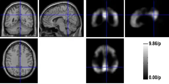
The goal of this example was to identify cognitively normal elderly people who were amyloid positive based on their brain imaging data. The dataset consisted of 64 normal control elderly subjects (43 female, 21 male) with an average age of 74 (standard deviation = 5.4; range: 65-89). A brain image was acquired for each subject with the value of each voxel reflecting the amount of amyloid deposition in the brain. There are 343,147 voxels in each image after the non-brain voxels were masked out. The input for the clustering analysis was a dataset with n = 64 subjects and p = 343,147 voxels per image for the analysis. We intended to classify the dataset into two clusters, so K is equal to 2. We applied the proposed method and the dataset were resampled 50 times.
A brain map of voxel (or variable) weights, which indicates their importance in distin-guishing clusters, was computed for each of these samples during the resampling. These weights were standardized for the different tuning parameters, which ranged from 305.56 to 383.89. A total of 50 brain maps were generated with one for each resampling run. As de-scribed in the methods section, the final weight for each voxel was computed as the average of the standardized weights across the 50 resampling runs. The image with the final voxel weights is shown as the right half in Figure ??, in which a brighter color means a bigger weight while a darker color means a smaller weight. On the left a high resolution Magnetic Resonance (MR) Image showed the corresponding brain anatomy. The slices shown here were representative of typical regions with amyloid deposition.
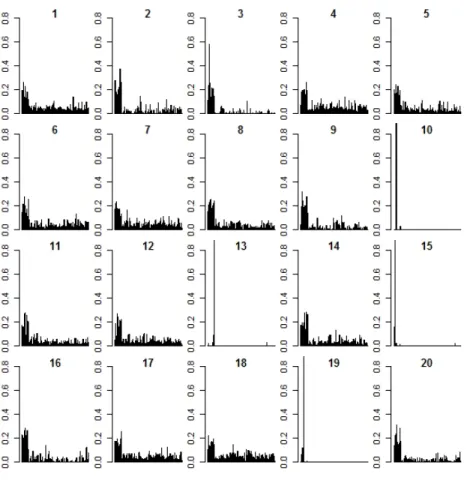
The range of the weights is from 0 to 9.86 fold of 1/p, where p = 343,147 and 1/p = 2.88×10⁻⁶. The voxel weights were bigger in the prefrontal, the precuneus, and the parietal cortex regions indicating that these regions were important for subgroupings while the voxel weights in the sensorimotor and cerebellar cortex were much smaller indicating they were not that important for the subgroupings. These findings were consistent with the distribution of amyloid deposition in the human brain across a spectrum of subjects and biologically meaningful.
Among all 64 subjects, there were 7 subjects identified as amyloid positive and 37 subjects identified as amyloid negative at the confidence level 100%. Another subject was identified as positive at a confidence level 84%. The remaining 19 subjects were negative at the confidence levels 98% (for four subjects), 96%(for one subject), 94% (for two subjects), 90% (for three
9.86/p
0.00/p
Figure 3: Voxel/Variable weights. (Left) Magnetic Resonance Image which shows the brain anatomy; (Right) The image with the final weights for each voxel (or each variable). The range of weights is 0 to 9.86 fold of 1/p, where p = 343,147 and 1/p = 2.88×10⁻⁶. The image dataset was resampled 50 times.
subjects), 88% (for four subjects), 84% (for one subject), 78% (for one subject), and 76% (for three subjects). These results indicates that there were 7 subjects who were always amyloid positive and 1 subject somewhat positive, and there were 37 subjects who were always amyloid negative, 5 who were very negative with confidence levels>95%, and 14 who were somewhat negative with a confidence level in the range of 76%−94%. In spite of the fact that the amyloid groups were not clearly separated because of these somewhat positive/negative subjects, all of the subjects were classified into a group with strong confidence with the confidence levels being ≥ 76% for the negative subjects and ≥ 84% for the positive ones. This may serve as evidence against the idea of a third cluster for these intermediate subjects. To further understand a potential classification of “amyloid positive”, we could examine the characteristics of the dataset with the information provided by the clustering results. For example, we could assess the difference between the somewhat positive subject against the group with seven always positive subjects or against the group with the fourteen somewhat negative subjects. We could also choose to compute cluster centers from the tight clusters with a confidence level threshold ≥ 95% and use these reliable cluster centers to predict membership for any additional PiB scans.
2.5 CONCLUSIONS AND DISCUSSION
The proposed method, “sparse k-means and resampling”, can achieve both variable selection and tight clusters for datasets with the property of “high-dimension, small sample size” (p n). The final standardized variable weights can serve as a more reliable metric to exclude the irrelevant variables and yield parsimonious clustering results. The confidence levels for the clustering results provided more information than the usual approach of dichotomizing results from clustering methods without resampling. These confidence levels can be used to construct tight clusters with different degrees of tightness and to potentially identify the degree of the overlap between the clusters. To date, this work is the first method to combine resampling with sparse clustering. This method is especially useful for neuroimaging datasets, where the small sample size is usually a concern.
The proposed method provides additional information on variable weights and clustering results through resampling. Bootstrapping was not used because bootstrapping resamples the data with replacement, which makes it very complicated to summarize the results across resampling runs. We illustrated the use of metrics such as the final standardized variable weight and the confidence level for the cluster results. Depending on the goal of the scientific question, other metrics may be more appropriate for summarizing the resampling results. For example, in the case of constructing rules for diagnostic tests, it may be of interest to find more reliable cluster centers and to use them for cluster membership prediction. In this case, the focus will be summarizing the cluster centers from the resampling results. Like sparse k-means, this method is most useful whenpn, but also works in the case ofp < n. One major limitation of this method is that resampling tends to be time-consuming. It is an inevitable trade off that we have to make to gain more confidence in the clustering results. The method does not perform as well when the underlying groups significantly overlap with each other and the number of variables, p, is much larger than the number of truly different variables, q. Prescreening of variables may be useful to decrease the number p before clustering is applied, and is a topic for future research. We have showed that the proposed method works well when the number of clusters is 2 or 3. We anticipate that its performance may be compromised when the number of clusters gets larger. For example, it may become very challenging to properly align the cluster centers from the different resampling runs.
We have also encountered the problems related to the tuning parameter choice based on gap statistic. The Witten and Tibshirani (2010) [35] paper pointed out that the performance of the gap statistic for selecting the tuning parameter was not always great. In our experience the gap statistic has worked well in choosing the tuning parameters in neuroimaging appli-cations. But when the default tuning parameter pool 1.2,0.9√p was used in Simulations 1 and 2, the tuning parameters that were either too small, or too large, yielded clustering results with unusually higher classification error rates. This was why we chose to use an adjusted tuning parameter pool in this paper. We have also been searching for methods that could potentially address this issue.
In summary, the proposed method of combining sparse clustering with resampling pro-vides an improvement over currently existing techniques. The use of a confidence metric, based on the observed proportion of times that an observation falls in a given cluster is extremely useful for assessing the potential classification of normal control subjects into “amyloid positive” and “amyloid negative” groups. These groupings are key for targeting future prevention strategies in Alzheimer’s disease.
3.0 TUNING PARAMETER CHOICE FOR SPARSE K-MEANS CLUSTERING
3.1 INTRODUCTION
Clustering is important in exploring and discovering distinct biological groups in the ear-lier stage of scientific studies when no definite group membership could be assigned to the observations. It can be used to establish rules for predicting memberships for additional ob-servations. Clustering methods with variable selection, also called sparse clustering, choose the variables that more accurately reflect the variability in the original dataset while dimin-ishing or eliminating the effects of less relevant variables on the clustering. The resulting clustering rules are more parsimonious, easier to interpret, and could yield a more desir-able prediction accuracy. This is true when p < n but it is more evident in the case of “high-dimension, low sample size” (pn).
Variable selection realized by penalties was first developed in linear regression. A very influential approach wasLasso[29], which stands for “Least absolute shrinkage and selection operator”. It was proposed by Tibshirani in 1996 and has been widely applied since then. For linear regression, an L1/Lasso penalty imposes an upper bound s to the summation of absolute values of the regression coefficients βi’s, i.e. Ppi=1|βi| ≤ s, where p is the
number of independent variables in the model. The algorithm minimizes the target function of the sum of squares with restrictions of this penalty. The resulting coefficients are then subject to shrinkage in absolute value (absolute shrinkage) or have a value of 0 (selection). When the coefficient is 0, the variable is not selected in the model. Solving for the problem can be regarded as convex optimization and solutions are obtained by applying the soft-thresholding operator because it satisfies the Karush-Kuhn-Tucker conditions [2,29]. Least
Angle Regression (LARS) was developed by Efron, Hastie, Johnstone and Tibshirani in 2002 to solve the Lasso in a much faster manner [5]. A further significant improvement in solving Lasso was coordinate descent algorithm [11, 9, 10, 37, 12]. These algorithms have evolved to be so efficient that the computing time is no longer a concern.
Lasso and related penalties have been applied to a wide range of traditional statisti-cal methods to realize variable selection. The resulting methods are statisti-called regularization methods. They have been applied to linear regression [29], generalized linear models [29], survival analysis [30], clustering [35, 27] and support-vector machine [14]. They have also been applied to dimension reduction methods such as principal component analysis [17, 36], canonical correlation analysis [36] and partial least squares [4]. Variants of penalties include the Grouped Lasso [38, 26], Elastic Net [41], Adaptive Lasso [40], Graphical Lasso [39, 9], Dantzig Selector [3] and others. A discussion of these penalties was given in [10, 31]. In this work we will focus on the application of these penalties in clustering and the tuning parameter choice.
Most of the clustering methods with variable selection are implemented with an L1 or Lasso penalty. A general framework for clustering was proposed by Witten and Tibshirani in 2010 [35]. It applied an L1 and an L2 restraint on k-means to realize variable selection, i.e. sparse clustering. The algorithm was implemented by an EM algorithm alternating between weighted k-means and convex optimization. The authors showed that it also works for hierarchical clustering and k-mediods clustering. These penalties were also applied in the model-based clustering framework. Pan and Shen in 2007 [27] proposed a penalized model-based clustering method, in which aLasso penalty and a modified BIC were used to realize model selection. The penalized mixture model assumes independence between variables and the same diagonal covariance matrix across clusters.
The sparse clustering method results depend on the choice of the tuning parameter [35] or the penalization parameter [27] (For simplicity reasons, we will only use the term “tuning parameter” from here on). For example in the Witten and Tibshirani paper [35] a larger tuning parameter usually allows for more of the variables to be selected for clustering and vice versa. The choice of the tuning parameter has been studied in regression and classification with cross-validation being the main approach. This method can not be easily
applied to clustering due to the lack of the true membership. Pan and Shen in 2007 [27] used a modified BIC to determine both the number of clusters and the tuning parameter. Witten and Tibshirani in 2010 [35] proposed using the gap statistic. Yet both of these methods rely on the correct specification of the tuning parameter pool.
We have observed that given a suboptimal pool the gap statistic method could choose a tuning parameter which yields poor performance when clustering, i.e. a high Classification Error Rate (CER). When this happens it usually chooses a tuning parameter that is too small or too large, hence too few, or too many, variables are chosen for clustering. This is more likely to occur when the overlap between the clusters is more substantial. In this work, we would like to draw attention to this phenomenon and also to propose using BIC for the choice of tuning parameter for the sparse k-means method proposed by Witten and Tibshirani in 2010.
3.2 GAP STATISTIC FOR TUNING PARAMETER CHOICE
The gap statistic was originally proposed by Tibshirani in 2001 [33] for the purpose of choosing the number of clusters when clustering is applied to a dataset and the number of clusters is unknown. The Witten and Tibshirani[2010] paper adopted it for the purpose of choosing the tuning parameter [35]. The definitions and notations in these two papers are different although the essence of it is the same. The gap statistic is defined to be the difference, i.e. gap, between the observed value and the expected value of the target function on the logarithm scale. In the Witten and Tibshirani[2010] paper, the target function in sparse k-means is to maximize the weighted Between-Cluster Sum of Squares (BCSS), which is defined as O(s) = p X j=1 wj 1 n n X i=1 n X i0=1 di,i0,j− K X k=1 1 nk X i,i0∈C k di,i0,j ! . (3.1)
The corresponding gap statistic is defined as
whereE[log(Ob(s)] is the expected value of the target function on the logarithm scale. The
expected target function value is obtained by permutation and will be discussed in detail next.
The permuted dataset is generated in a way such that the values in each column are randomly chosen from the corresponding column in the original dataset. There are B per-muted datasets. These perper-muted datasets are supposed to reflect the reference, or the null, distribution. For a given tuning parameter, sparse clustering will be applied to each of these datasets and a value of the target function can be calculated. The average of them
1
B
PB
b=1log(Ob(s)) is the expected value of the target function. Simply put, it is the average
of the weighted BCSS for the B permuted dataset. Thus the gap statistic is
gap(s) = log(O(s))− 1 B B X b=1 log(Ob(s)). (3.3)
We will compute the gap statistic for every choice in the tuning parameter pool. Intu-itively, the tuning parameter s∗ for which the clustering achieves the largest gap statistics is chosen for sparse clustering. The default pool for tuning parameter choice is 1.2,0.9√p.
3.3 TUNING PARAMETER CHOICE IN PENALIZED MODEL-BASED CLUSTERING
3.3.1 Model-based Clustering
For a dataset,Xn×p, with n observations andpvariables observed for each observation,
sup-pose that the number of clusters isK. Model-based clustering assumes that each observation of the dataset is drawn from a finite mixture distribution. Assume that each underlying clus-ter Ck follows a multivariate distribution fk(x;θk), where θk is a vector of the parameters
specifying the distribution. The K clusters form a mixture of these multivariate distribu-tions, which is a finite mixture distribution and can be denoted asf(x;θ) =PK
k=1πkfk(x;θk). Here πk is the probability of one observation belongs to the kth cluster and
PK
k=1πk = 1.
θk, which maximize the likelihood of observing the dataset. The log-likelihood can be written as logL(θ) = n X i=1 log[ K X k=1 πkfk(xi;θk)], (3.4)
where xi, i= 1,2, . . . , n, is the ith observation in the dataset, Xn×p.
EM algorithms are used to obtain the solutions as described in McLachlan and Peel[2002] [23, 24] and Fraley and Raftery[2002] [8].
3.3.2 Penalized Model-based Clustering
Under the model-based clustering framework and assuming a multivariate normal distribu-tion the Pan and Shen [2007] paper proposed a penalized model-based clustering approach [27]. It assumes that the dataset is sampled from a finite mixture of multivariate normal distributions. The method further assumes that the covariance for each component is a di-agonal matrix and they hold the same across all components. Recall that the p-dimensional multivariate normal distribution density with mean µ and covariance Σ is
f(x;µ,Σ) = 1 (2π)p/2|Σ|12 exp −1 2(x−µ) 0 Σ−1(x−µ) . (3.5)
Hence, each component of the mixture distribution can be denoted as
fk(x;µk, V) = 1 (2π)p/2|V|12 exp −1 2(x−µk) 0 V−1(x−µk) , (3.6)
where µk is the mean for the kth component; the covariance matrix is the same for each
component, it is V =diag(σ2
1, σ22, . . . , σp2) and |V| 1 2 =Qp
j=1σj. The penalized log-likelihood is
logL(θ) = n X i=1 log[ K X k=1 πkfk(xi;θk)]−hλ(θ), (3.7)
wherehλ(θ) = λPKk=1Ppj=1|µkj|. This L1-penalty term is imposed so that the mean values
µkj for the finite mixture distribution are subject to shrinkage. Similarly an EM algorithm
is used to solve for the clustering memberships and the distribution parameters. Details are described in [27]. When all theµkj values for the samej are estimated to be zeroes, thejth
3.3.3 BIC for Tuning Parameter Choice
The Fraley and Raftery [1998] paper [7] proposed to use Bayesian Information Criterion (BIC) [28] for model selection in the framework of model-based clustering, where
BIC =−2 logL( ˆΘ) +dlog(n), (3.8)
in which ˆΘ is the Maximum Likelihood Estimator (MLE) and d is the number of parameters to estimate.
For penalized model-based clustering since the models being compared may have dif-ferent numbers of parameters due to the degree of regularization, i.e. the value of the tuning/penalization parameter, a modified BIC is used for model selection. The modified BIC is defined as
BICe=−2 logL( ˜Θ) +delog(n), (3.9)
where ˜Θ is the Maximum Penalized Likelihood Estimator (MPLE) andde is the number of
parameters to estimate in the regularized model. Since the parameters to estimate without regularization areπk’s, σj’s, and µkj’s and
PK
k=1πk= 1, the number of parameters is
K+p+Kp−1. The number of free parameters is de =K+p+Kp−1−q where q is the
number of zero µkj’s.
The modified BIC BICe was used to determine both the number of clusters and the
tuning parameter. A tuning parameter pool will be specified as a vector with Nλ possible
tuning parameter values and a small possible number of K’s, say NK, will also be
pre-specified. Then penalized model-based clustering will be fitted to the dataset with every of the Nλ×NK scenarios. The model with the best BIC will be chosen from all theseNλ×NK
3.4 PROBLEMATIC RESULTS USING GAP STATISTIC
The Witten and Tibshirani[2010] paper pointed out that “the performance of the gap statis-tic” “for selecting the tuning parameter is mixed” [35]. In our experience the gap statistic has worked well in choosing the tuning parameters in neuroimaging applications either when p < nfor a dataset with regional outcome measures or whenpn with voxel-wise outcome measures. But when the default tuning parameter pool 1.2,0.9√p was used in the first simulation in the Witten and Tibshirani[2010] paper, the tuning parameters were chosen to be too small or too large in certain scenarios that yielded clustering results with higher CER values. We will dissect the problem in more detail next.
This simulation set up is similar to that outlined in section 2.3.2. The simulation was originally chosen [35] to compare sparse k-means and k-means. There are three groups in the original dataset with 20 observations in each group. The groups were different in the first q= 50 variables while not distinguishable in the remaining p−q variables, where p = 50, 200, 500 and 1000. The firstq = 50 variables were different in a way that the first group was sampled from the normal distributionN(−µ,1), the second group fromN(0,1), and the third group from N(µ,1), where µ = 0.6, 0.7, 0.8, 0.9 and 1.0. The value µ is an indicator of the overlap between the groups in the q variables. The overlap is most substantial when µ= 0.6 and decreases asµ gets bigger. The groups were best separated whenµ= 1.0.
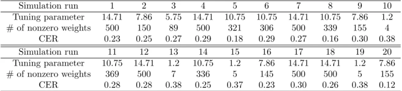
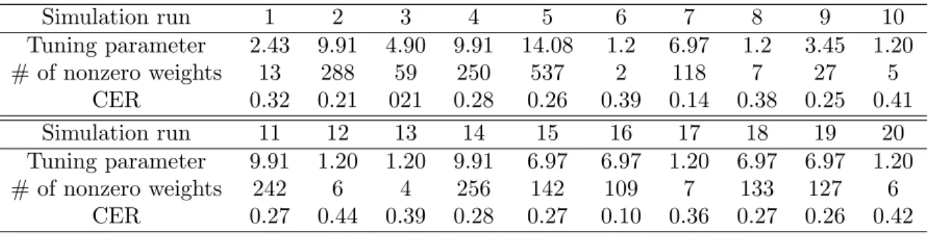
Table 5: Tuning parameter choice for µ= 0.6 and p= 500
Simulation run 1 2 3 4 5 6 7 8 9 10 Tuning parameter 14.71 7.86 5.75 14.71 10.75 10.75 14.71 10.75 7.86 1.2 # of nonzero weights 500 150 89 500 321 306 500 339 155 4 CER 0.23 0.25 0.27 0.29 0.18 0.29 0.27 0.16 0.30 0.38 Simulation run 11 12 13 14 15 16 17 18 19 20 Tuning parameter 10.75 14.71 1.2 10.75 1.2 7.86 14.71 14.71 1.2 7.86 # of nonzero weights 369 500 7 336 5 145 500 500 5 155 CER 0.28 0.28 0.38 0.25 0.37 0.23 0.30 0.26 0.38 0.12
The sparse k-means method proposed by Witten and Tibshirani requires that the tuning parameter is in the range 1,√p [35]. The default tuning parameter pool is specified as 1.2,0.9√p for the sparse k-means R routine implemented by the authors with the default number of tuning parameters in the pool being 10. The tuning parameters were chosen