Pre-processing feature selection for improved C&RT models for oral absorption

Pr

e

-pr

oce

ss

in

g

fea

tur

e

se

le

cti

o

n

“T

w

o

st

ag

e

app

roac

h

”

No

p

re

-p

roce

ss

in

g

“One

st

ag

e

ap

p

ro

ach

”

Oral ab

sorp

tion

Q

SAR Mod

el

s

V

s.

ACS Paragon Plus Environment

Pre-processing feature selection for improved C&RT models for oral absorption

1

Danielle Newbya, Alex. A. Freitasb, Taravat Ghafouriana,c*

2

a_{Medway School of Pharmacy, Universities of Kent and Greenwich, Chatham, Kent, ME4} 3

4TB, UK 4

b_{School of Computing, University of Kent, Canterbury, Kent, CT2 7NF, UK} 5

c _{Drug Applied Research Centre and Faculty of Pharmacy, Tabriz University of Medical}

6

Sciences, Tabriz, Iran 7

* Corresponding Author, Email: [email protected]; Tel +44(0)1634 202952; Fax 8 +44 (0)1634 883927 9 10 11 12 13 14 15 16 17 18 19 20 21 22 23 24 25 2 3 4 5 6 7 8 9 10 11 12 13 14 15 16 17 18 19 20 21 22 23 24 25 26 27 28 29 30 31 32 33 34 35 36 37 38 39 40 41 42 43 44 45 46 47 48 49 50 51 52 53 54 55 56 57 58

Abstract

26

There are currently thousands of molecular descriptors that can be calculated to represent a 27

chemical compound. Utilising all molecular descriptors in Quantitative Structure-Activity 28

Relationships (QSAR) modelling can result in overfitting, decreased interpretability and thus 29

reduced model performance. Feature selection methods can overcome some of these 30

problems by drastically reducing the number of molecular descriptors and selecting the 31

molecular descriptors relevant to the property being predicted. In particular, decision trees 32

such as C&RT, although they have an embedded feature selection algorithm, can be 33

inadequate since further down the tree there are fewer compounds available for descriptor 34

selection and therefore descriptors may be selected which are not optimal. In this work we 35

compare two broad approaches for feature selection: (1) a “two-stage” feature selection 36

procedure, where a pre-processing feature selection method selects a subset of descriptors, 37

and then classification and regression trees (C&RT) selects descriptors from this subset to 38

build a decision tree; (2) a “one-stage” approach where C&RT is used as the only feature 39

selection technique. These methods were applied in order to improve prediction accuracy of 40

QSAR models for oral absorption. Additionally, this work utilises misclassification costs in 41

model building to overcome the problem of the biased oral absorption datasets with more 42

highly-absorbed than poorly-absorbed compounds. In most cases the two stage feature 43

selection with pre-processing approach had higher model accuracy compared with the one 44

stage approach. Using the top 20 molecular descriptors from random forest predictor 45

importance method gave the most accurate C&RT classification model. The molecular 46

descriptors selected by the five filter feature selection methods have been compared in 47

relation to oral absorption. In conclusion, the use of filter pre-processing feature selection 48

methods and misclassification costs produce models with better interpretability and 49

predictability for the prediction of oral absorption. 50

Keywords:

51

Oral absorption, intestinal absorption, in silico, classification, feature selection, QSAR 52 53 2 3 4 5 6 7 8 9 10 11 12 13 14 15 16 17 18 19 20 21 22 23 24 25 26 27 28 29 30 31 32 33 34 35 36 37 38 39 40 41 42 43 44 45 46 47 48 49 50 51 52 53 54 55 56 57 58

1. Introduction

54

The cost of bringing a drug to the market keeps on increasing 1, 2_{. The expense is likely to rise}

55

further with higher costs of everything from consumables to clinical studies and also tighter 56

regulations governing acceptance of oral drugs on the market 3. Although there has been a

57

successful effort to reduce compound attrition rates by incorporating pharmacokinetic (PK) 58

assays in a high throughput manner earlier in drug discovery, compounds are now failing for 59

other reasons as well as poor PK such as efficacy and toxicity 4. There is specific interest in

60

predicting the intestinal absorption of new chemical entities (NCEs) as the oral route is the 61

dominant route of drug delivery due to ease of administration and patient acceptance 5, 6_{. In}

62

silico modelling of intestinal absorption using QSAR (Quantitative Structure-Activity 63

Relationships) can be used as a cost effective strategy to remove unsuitable compounds based 64

on physicochemical properties and chemical structure alone. Moreover, in silico modelling

65

can be used in tandem with high throughput assays in drug discovery and act as a guide to 66

select appropriate assays that will help understand the mechanistic absorption properties of 67

compounds 7.

68

QSAR involves the mathematical relationships between a molecular structure and biological 69

activity. However this relationship cannot be determined directly, therefore molecular 70

descriptors that describe the chemical structure are calculated to derive relationships between 71

the molecular descriptors and activity. Molecular descriptors are numerical representations of 72

the chemical structure. Molecular descriptors can be classed as 0, 1, 2, 3 and 4D groups 8_.

73

Simple 0D descriptors are counts of atom and bonds in structure such as molecular weight 74

and number of hydrogen atoms in a molecule. Molecular descriptors that count structural 75

fragments, atomic properties or fingerprints are classed as 1D. Examples of 1D are number of 76

hydrogen bond donors or acceptors. Topological descriptors based on the 2D structure of the 77

molecule are predicted using graph theory, vectors and indices, and examples include the 78

kappa shape, chi connectivity indices 9 and topological polar surface area 10. More

79

complicated molecular descriptors such as 3D and 4D require the 3D coordinates of the 80

structure. 3D descriptors are geometric descriptors and there are two types based on the 81

internal or external orientation properties of the molecule. Good examples of 3D descriptors 82

are energies relating to the orbitals of the atoms in the compound such as the lowest

83

unoccupied molecular orbital (LUMO) and the highest occupied molecular orbital (HOMO) 84

energies. These molecular descriptors are derived from quantum chemistry theories and relate 85 2 3 4 5 6 7 8 9 10 11 12 13 14 15 16 17 18 19 20 21 22 23 24 25 26 27 28 29 30 31 32 33 34 35 36 37 38 39 40 41 42 43 44 45 46 47 48 49 50 51 52 53 54 55 56 57 58

to the reactivity of the compound. Finally 4D descriptors are based on the 3D structure but 86

take into account the different flexibilities of the structure 8_.

87

In order to produce a model that is robust and high in predictive power, a wide choice of

88

molecular descriptors is very important. Identifying the relevant descriptors correlating with 89

intestinal absorption can be carried out using statistical feature selection methods although, 90

additionally, educated assumptions can be made about physiological and physicochemical 91

factors that influence the process of oral absorption to choose the useful descriptors 11.

92

Feature selection is used frequently in QSAR and data mining to selectively minimise the 93

number of independent variables (molecular descriptors) used to accurately describe the 94

dependent variable – i.e., absorption 12. Feature selection is important for numerous reasons.

95

Firstly, fewer molecular descriptors increase interpretability and understanding of resulting 96

models 13, 14. Secondly feature selection can provide improved model performance for the

97

prediction of new compounds 15, 16. Finally, it can reduce the risk of overfitting from noisy

98

redundant molecular descriptors 17.

99

Feature selection can be split into two broad categories: data pre-processing or embedded 100

methods. Data pre-processing feature selection involves reduction of the number of molecular 101

descriptors before model building, unlike embedded methods that incorporate the feature 102

selection into the training and building of the model 17, 18. Data pre-processing techniques can

103

be further split into filter and wrapper techniques. Filter techniques usually involve 104

calculating a relative score of the molecular descriptors and ranking them in order of best 105

score, and the descriptors that are at the top of the list are then used as input for classification. 106

Examples of these are chi square and information gain. Wrapper techniques consider a 107

number of subsets of molecular descriptors, evaluate each of these based on the predictive 108

performance of a classification model built from that descriptor subset and eventually select 109

the descriptor subset with the best predictive performance 19. In comparison of filter and

110

wrapper methods, there are advantages and disadvantages. The choice of method depends on 111

many things such as interpretability, predictability and computational cost. 112

Filter methods offer a fast and simple way to select important descriptors. In addition, 113

because they are independent of the classification algorithm, the score for each descriptor 114

only needs to be calculated once, and the selected descriptors can be used as input for a 115

variety of classification algorithms. A disadvantage of univariate filter methods is they fail to 116

account for interactions between independent variables as most measure the correlation 117 2 3 4 5 6 7 8 9 10 11 12 13 14 15 16 17 18 19 20 21 22 23 24 25 26 27 28 29 30 31 32 33 34 35 36 37 38 39 40 41 42 43 44 45 46 47 48 49 50 51 52 53 54 55 56 57 58

between the dependent variable and each independent variable separately. This can be 118

overcome by multivariate methods which take into account independent variable interactions. 119

Wrapper techniques on the other hand are usually more computationally expensive, but 120

unlike many univariate filter techniques, they take into account independent variable 121

interactions 17, 18_{. In addition, hybrid filter and wrapper methods have also been developed as}

122

successful feature selection techniques 20

123

Most oral absorption models in the literature have utilised feature selection methods either in 124

pre-processing or in model development. There are many types of research in the literature 125

that focus on different issues of oral absorption modelling; e.g. those that focus on obtaining 126

a high predictive model with the feature selection not as the primary focus, but just as a part 127

of the modelling process 21; and those that compare different feature selection techniques and

128

compare the molecular descriptors chosen by the different techniques 11, 20. However, an

129

underlying problem of oral absorption models in the literature is that they were developed 130

using current oral absorption datasets in the literature which are highly biased towards the 131

prediction of highly-absorbed compounds 21-24. This is due to availability of more data on

132

marketed drugs which are mostly highly-absorbed in contrast with data on compound and 133

drug candidates that never made into the market and failed during drug discovery. The 134

models in this case may predict high absorption rate for poorly-absorbed compounds, i.e. 135

false positives. This is not an ideal scenario as in drug discovery more compounds are now 136

poorly-absorbed due to higher lipophilicity and poor aqueous solubility of current drug

137

candidates 25, 26.

138

Two methods have been studied previously to overcome the problem of biased oral datasets 139

that show the effect of data distribution in the training sets for regression and classification. 140

Firstly under-sampling the majority class, highly-absorbed compounds, to create a balanced 141

training set with the same number of poorly and highly-absorbed compounds 27. The second

142

technique utilises the whole biased dataset but applies misclassification costs to reduce false 143

positives 28. The use of higher misclassification costs for model development should improve

144

the predictive power of the model built with the molecular descriptor subsets chosen by 145

appropriate feature selection methods. 146

This work investigates five pre-processing filter feature selection techniques for selecting 147

subsets of molecular descriptors. The comparison of these different feature selection 148

techniques is anticipated to give an idea of the relative abilities of the different techniques 149 2 3 4 5 6 7 8 9 10 11 12 13 14 15 16 17 18 19 20 21 22 23 24 25 26 27 28 29 30 31 32 33 34 35 36 37 38 39 40 41 42 43 44 45 46 47 48 49 50 51 52 53 54 55 56 57 58

based on their prediction ability on the validation set. Furthermore, we compare two broad 150

approaches for feature selection: (1) a “two-stage” feature selection procedure, where in the 151

first stage a pre-processing feature selection method selects a subset of descriptors, and in the 152

second stage classification and regression trees (C&RT), which is itself an embedded feature 153

selection method, selects a subset of the descriptors selected by the filter technique to build a 154

decision tree; (2) a “one-stage” approach where C&RT is used as the only feature selection 155

technique, without using data pre-processing feature selection methods. A comparison 156

between these two approaches could indicate the usefulness of pre-processing feature 157

selection for C&RT analysis. Additionally, this work utilises misclassification costs in model 158

building to overcome the problem of biased datasets. This work offers an investigation of 159

feature selection techniques which reduces the number of molecular descriptors, increasing 160

interpretability of resulting models and combined with this the use of misclassification costs 161

in model development to increase model predictability when analyzing a biased dataset. 162

Therefore this work offers a novel combination of pre-processing feature selection combined 163

with misclassification costs to develop models for biased oral absorption datasets. 164

2. Methods and Materials

165

2.1 Dataset and Misclassification Costs

166

The published dataset of Hou et al21 containing %HIA (Percent Human Intestinal Absorption)

167

data for 645 drugs and drug-like compounds was utilised for development and optimisation 168

of models. An additional set of data was collated from literature to serve as the external 169

validation set. The %HIA values and references for the external validation set can be found in 170

the Supporting Information. 171

All the compounds in Hou et al’s data set were sorted by ascending %HIA values and then by 172

logP values. The %HIA ascending values were put into groups of six then 5/6th of these 173

compounds were placed randomly in the training set and the remaining into the parameter 174

optimisation set (internal test set). The training set was used to train the model in C&RT; the 175

parameter optimisation set was used to obtain the best parameters for the models. In addition, 176

the external validation set was used to show the predictive ability of the models created with 177

an unseen validation set. All compound sets had similar data distributions of highly and 178

poorly-absorbed compounds to create a fairer more controlled validation of the models. The 179 2 3 4 5 6 7 8 9 10 11 12 13 14 15 16 17 18 19 20 21 22 23 24 25 26 27 28 29 30 31 32 33 34 35 36 37 38 39 40 41 42 43 44 45 46 47 48 49 50 51 52 53 54 55 56 57 58

exact number of compounds in the training, parameter optimisation and validation set are 180

shown in Table 1.

181

Table 1. Numbers of Compounds for training, parameter optimisation and validation sets 182

Data Set Number of

compounds (N)

Training set 534

Parameter optimisation set 107

Validation set 48

183

As stated previously the data set is highly skewed with many more highly-absorbed than 184

poorly-absorbed compounds. Therefore any model generated using this biased dataset will be 185

better at predicting highly-absorbed than poorly-absorbed compounds and there will be more 186

misclassified poorly-absorbed compounds (false positives). To overcome this problem 187

applying a higher misclassification cost to the poorly-absorbed misclassification (false 188

positive) will reduce the number of false positives and increase overall prediction accuracy. 189

In a previous investigation it was shown that applying misclassification costs to the 190

prediction of poorly-absorbed compounds improved the predictive power especially for 191

poorly-absorbed compounds by overcoming the distribution bias of the dataset 28. In this

192

work, in order to assign an objective number for the overall misclassification cost, we have 193

used the class distribution of the highly and poorly-absorbed compounds. Therefore we have 194

used a misclassification factor of four to one, for low and high classes, respectively. 195

2.2 Molecular descriptors

196

A variety of different software packages were used to compute molecular descriptors; they 197

include TSAR 3D v3.3 (Accelrys Inc.), MDL QSAR (Accelrys Inc.), MOE (Chemical 198

Computing Group Inc.) v2010.10 and Advanced Chemistry Development ACD Labs/ LogD 199

Suit v12. A total of 204 descriptors were initially used in this study before applying feature 200

selection methods. 201

2.3 Classification and Regression Trees (C&RT)

202

Classification of the compounds using C&RT analysis was carried out using STATISTICA 203

v11 (StatSoft Ltd). Compounds were placed into categorical classes of ‘high’ or ‘low’ 204

according to the observed %HIA value in the dataset. The threshold for the classes was 50%; 205

therefore any compounds with %HIA ≥ 50% was assigned to the ‘High’ class and any 206

compound with a %HIA less than 50% was assigned to the ‘Low’ class. 207 2 3 4 5 6 7 8 9 10 11 12 13 14 15 16 17 18 19 20 21 22 23 24 25 26 27 28 29 30 31 32 33 34 35 36 37 38 39 40 41 42 43 44 45 46 47 48 49 50 51 52 53 54 55 56 57 58

C&RT analysis is a statistical technique that uses decision trees to solve regression and 208

classification problems 29. For this work, the dependent variable (HIA Class) was categorical

209

and classification trees were produced which classed compounds either ‘high’ or ‘low’ 210

absorption. For this work the stopping factors were minimum number of compounds for 211

splitting at 30 based on preliminary experiments. This enables pruning of the tree and 212

prevents over-fitting of the decision tree 29, 30.

213

For this work, HIA Class was set as the dependent categorical variable and either all 203 214

molecular descriptors or a subset of these selected by various feature selection methods were 215

selected as continuous independent variables. The analyses also included one categorical 216

independent variable, N+ group, the indicator variable for presence or absence of quaternary 217

ammonium. If there were any trees with only one compound in the terminal nodes, manual 218

pruning was carried out to prevent this final split so that no terminal nodes contained only 219

one compound. All other settings used were default setting defined by the software. 220

It must be noted that C&RT performs embedded feature selection; therefore in this work we 221

are also investigating the use of feature selection methods in a pre-processing phase, before 222

inputting the descriptor subset into C&RT. By carrying out data pre-processing feature 223

selection the methods can avoid C&RT’s drawback of ‘data fragmentation’. In other words, 224

as the decision tree is built and compounds split into smaller nodes there are fewer 225

compounds to split; therefore, the selection of descriptors in that local node becomes less 226

statistically reliable. Figure 1 shows the work flow of this investigation and how the

pre-227

processing feature selection selects molecular descriptors as input for C&RT analysis 228

compared to the embedded C&RT approach. 229 230 2 3 4 5 6 7 8 9 10 11 12 13 14 15 16 17 18 19 20 21 22 23 24 25 26 27 28 29 30 31 32 33 34 35 36 37 38 39 40 41 42 43 44 45 46 47 48 49 50 51 52 53 54 55 56 57 58

Figure 1: Workflow for molecular descriptor generation for pre-processing feature

231

selection and embedded C&RT analysis

232

2.4 Missing values

233

Missing values for molecular descriptors can be a problem when building QSAR models. 234

Depending on the software, procedures used to overcome the problems of missing values will 235

vary 20, 31. For example, with general C&RT analysis in STATISTICA any compounds with

236

missing values for certain molecular descriptors will be removed at the tree root. This means 237

that there are fewer compounds used to build the C&RT models and the possibility of 238

reducing the chemical coverage of the resulting QSAR model. In comparison, interactive 239

trees will remove chemical compounds from the decision tree on a case by case basis, so only 240

when that particular molecular descriptor is picked in the C&RT analysis will the chemical 241

compounds be removed. Missing molecular descriptors values for compounds can identify 242

patterns relating to certain functional groups or structural features that give rise to the missing 243

values. In this work it was noted that compounds that contained a permanent quaternary 244

ammonium ion had more missing descriptor values than other compounds in the dataset. 245

Therefore, an indicator variable that described the permanent positive nitrogen (YES/NO) 246

was calculated. Molecular descriptors that are difficult to compute and result in missing 247

values may not be suitable to be used in resulting models as the molecular descriptors may 248

not be able to be calculated for new compounds, leading to poor performance of the model

249

for classification of these compounds. Therefore, we removed all molecular descriptors that 250

had 10 or more missing values based on preliminary work, and therefore had a final number 251

of 204 descriptors available for feature selection techniques. 252

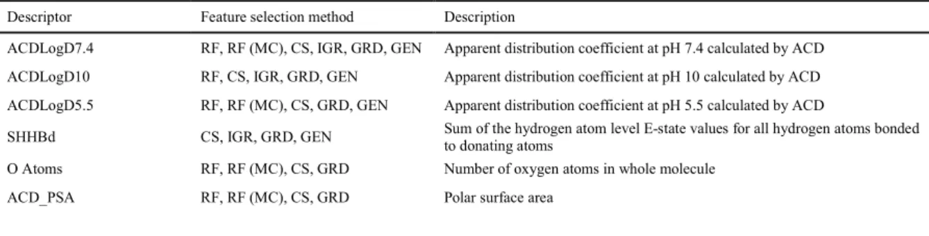
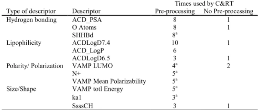
2.5 Feature Selection

253

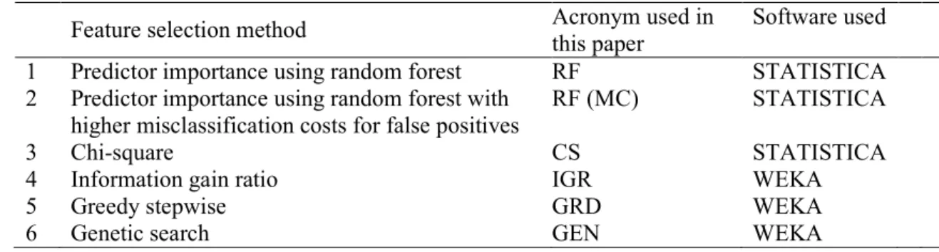
We used feature selection methods in pre-processing step to reduce the number of molecular 254

descriptors to a smaller subset that accurately describes the dependent variable, in this case 255

HIA Class. The software used for feature selection was STATISTICA v11 and WEKA v 3.6 256

32_{. The feature selection techniques to select molecular descriptors for the classification}

257

models of oral absorption are shown in Table 2. The descriptors selected by the feature

258

selection techniques in Table 2 were used as input by C&RT which then performed further

259

(embedded) feature selection (Figure 1).

260 261 262 2 3 4 5 6 7 8 9 10 11 12 13 14 15 16 17 18 19 20 21 22 23 24 25 26 27 28 29 30 31 32 33 34 35 36 37 38 39 40 41 42 43 44 45 46 47 48 49 50 51 52 53 54 55 56 57 58

Table 2. Pre –processing feature selection methods utilised in this work 263

Feature selection method Acronym used in

this paper

Software used

1 Predictor importance using random forest RF STATISTICA

2 Predictor importance using random forest with

higher misclassification costs for false positives

RF (MC) STATISTICA

3 Chi-square CS STATISTICA

4 Information gain ratio IGR WEKA

5 Greedy stepwise GRD WEKA

6 Genetic search GEN WEKA

264

It is also important to define which parts of dataset were used for the different feature 265

selection techniques. The training set is used by all methods; however, for the filter methods 266

CS, IGR, GRD and GEN the parameter optimisation set was combined with the training set 267

to carry out feature selection using these techniques. For random forest and C&RT 268

(embedded feature selection) the training set was used to train the model and separately the 269

parameter optimisation set was used to obtain optimal parameters for the method (Figure 2).

270

271

Figure 2. Compound sets were used for pre-processing and embedded feature selection.

272

In this work for methods RF, CS, IGR the top 20 molecular descriptors were selected based 273

on the highest values of the descriptor scoring function. Other numbers of selected molecular 274

descriptors were tried; however, based on the C&RT analysis results on the parameter 275

optimisation set, the top 20 descriptors gave the highest classification accuracy and was 276 selected. 277 2 3 4 5 6 7 8 9 10 11 12 13 14 15 16 17 18 19 20 21 22 23 24 25 26 27 28 29 30 31 32 33 34 35 36 37 38 39 40 41 42 43 44 45 46 47 48 49 50 51 52 53 54 55 56 57 58

2.5.1 Predictor importance ranking using Random forest (RF) 278

Random forest generates a set of decision trees based on random subsets of compounds and 279

descriptors in the training set. The ensemble of decision trees vote based on the individual 280

tree results and then the majority vote for a particular compound determines the classification 281

of that compound 33, 34.

282

This method was carried out for the training set and the parameters of the analysis were 283

optimised using the parameter optimisation set. The top 20 descriptors based on a ranking 284

function called predictor importance in STATISTICA were obtained from the selected model. 285

In STATISTICA software, for every molecular descriptor, the drop in each node impurity 286

(delta) is summed for all nodes in the trees and expressed relative to the largest sum – i.e. the 287

most significant descriptor. The delta is calculated for every descriptor (even if not used in 288

the node for the splitting of the tree) and summed for every node and tree produced in the 289

forest. The larger the delta the more significant the molecular descriptor is. The final summed 290

delta value for every descriptor is normalized against the most important molecular descriptor 291

and therefore expressed relative to the molecular descriptors with the largest delta. This 292

means that important molecular descriptors that may not have been picked to be in the trees 293

may still appear in the final predictor importance table. 294

Optimization of the random forest method was carried out based on the plot of 295

misclassification error on the parameter optimisation set vs. the number of trees. The 296

misclassification rate is the number of misclassified compounds divided by the total number 297

of compounds. The lower the misclassification rate for the parameter optimisation set, the 298

better the model. Based on the misclassification rate, the optimum number of trees was 299

selected and used to repeat the analysis again with the new optimized value. The maximum 300

number of levels for each tree was set to three. The software default value of eight was used 301

for the number of molecular descriptors used in each tree. For random forest there was an 302

option to apply misclassification costs, therefore two sets of molecular descriptors were 303

selected using this technique: a descriptor set selected using equal misclassification costs 304

(RF) and a descriptor set selected using a misclassification cost ratio of 4:1 for false 305

positives: false negatives (RF (MC)). 306

2.5.2 Chi Square (CS) 307

In STATISTICA the CS function can be calculated and molecular descriptors ranked 308

accordingly. CS is a statistical measure of the association (or dependence) between two 309 2 3 4 5 6 7 8 9 10 11 12 13 14 15 16 17 18 19 20 21 22 23 24 25 26 27 28 29 30 31 32 33 34 35 36 37 38 39 40 41 42 43 44 45 46 47 48 49 50 51 52 53 54 55 56 57 58

categorical variables 35. The greater the CS value, the more statistically significant the 310

molecular descriptor is in relation to the %HIA class, therefore allowing the most statistically 311

important molecular descriptors to be ranked. The main drawback of using CS as well as 312

many other filter techniques is that it is a univariate feature selection method; therefore it 313

does not take into account interactions between the molecular descriptors. This could be a 314

potential issue in relation to intestinal absorption, where there are many interlinking factors 315

influencing absorption with many molecular descriptors describing them 6, 36. CS is an

316

association measure for categorical descriptors, therefore there may be problems when 317

continuous variables are used that contain a large spread of numerical values, since the 318

conversion of numerical variables into categorical ones (required for the use of the chi square 319

measure) may lose relevant information. The software default number of bins (ten) was used 320

for chi square discretizing of the molecular descriptors. 321

2.5.3 Information gain ratio (IGR) 322

Information gain ratio is a normalised function of the information gain feature selection 323

method developed by Quinlan37 _{as part of the ID3 (Iterative Dichotomiser) decision tree}

324

algorithm. This feature selection method is used to split the decision tree into nodes and 325

identify molecular descriptors that are the best for the individual splits 37. Information gain

326

works to minimise the information needed to classify compounds into resulting nodes. It is 327

the difference between the original information (before the data is spilt) and the new 328

information produced after using the molecular descriptor to split the training set data. This 329

difference is the gain of information achieved by using a specific molecular descriptor, 330

therefore the molecular descriptor with the highest gain is the one used for the split 14.

331

Information gain ratio was first described by Quinlan38 _{in the context of the C4.5 algorithm,}

332

which superseded ID3. Information gain ratio overcomes the bias towards selecting those 333

molecular descriptors with many numerical values by normalising the information gain. The 334

higher the ratio value the better the molecular descriptor for the split. This feature selection 335

technique was carried out using WEKA 3.6. 336

2.5.4 Greedy Stepwise (GRD) 337

The previous feature selection methods are based on ranking the molecular descriptors based 338

on a certain criteria and do not take into account the interactions between the molecular 339

descriptors. Therefore two additional feature selection methods were used that utilise a search 340

method which takes molecular descriptor interaction into account as well as the correlation 341

with HIA class. These methods seek to maximise the correlation between HIA and the 342 2 3 4 5 6 7 8 9 10 11 12 13 14 15 16 17 18 19 20 21 22 23 24 25 26 27 28 29 30 31 32 33 34 35 36 37 38 39 40 41 42 43 44 45 46 47 48 49 50 51 52 53 54 55 56 57 58

molecular descriptors being tested, and minimise correlations between the molecular 343

descriptors. 344

The first of these methods is greedy stepwise, which is a forward stepwise feature selection 345

method 39. This is a local search method that firstly considers all the molecular descriptors

346

and picks the best one – i.e., the one that correlates with HIA class. It then starts again with 347

all the remaining molecular descriptors, and picks the best molecular descriptor that pairs 348

with the previously selected molecular descriptor in relation to HIA class. The iterations carry 349

on until a local maximum is reached. Due to the nature of this technique only a local search 350

can be carried out based on the molecular descriptor(s) selected in all the previous iterations, 351

therefore the potential for a global search of all the different possible subsets is limited, and 352

promising regions of molecular descriptor space can be missed 15. To guide the greedy search

353

in the feature selection process, in the WEKA software an evaluator is used. The evaluator 354

function used was correlation-based feature selection subset evaluator (CfssubsetEval). This 355

evaluator not only aims to maximise the correlation between the best molecular descriptors 356

and HIA class, but also to minimise the correlation or redundancy between the descriptors for 357

the search subsets generated. 358

2.5.5 Genetic Search (GEN) 359

GEN is a filter (rather than wrapper) version of the genetic algorithm 40. Genetic algorithm

360

(GA) was first created by Holland41_{, although the concept of genetic algorithm was being}

361

researched before this. Now termed generally as an evolutionary algorithm, GA mimics the 362

process of natural evolution. An initial population is created containing random candidate 363

solutions. In the context of this work, a candidate solution is a molecular descriptor subset. 364

Each candidate solution is evaluated in terms of its fitness (quality), and candidate solutions 365

are then selected to be reproduced and to undergo modifications with a probability 366

proportional to their fitness values. The process of selecting “parent” candidate solutions 367

based on fitness and producing “offspring” solutions that are based on the parents is 368

iteratively performed for a number of iterations, so that the population of candidate solutions 369

gradually evolves towards better and better candidate solutions. 41. In this work we have

370

utilised the genetic search feature selection method using WEKA software 42_{. This method}

371

carries out a global search in the ‘molecular descriptor space’ to find the best subset of 372

molecular descriptors relating to HIA class, guided by a subset evaluator that generates a 373

numerical value of ‘fitness’ (quality) of any given feature subset. Like with the greedy search 374

technique, the evaluation function used for the genetic search method was ‘CfssubsetEval’. 375 2 3 4 5 6 7 8 9 10 11 12 13 14 15 16 17 18 19 20 21 22 23 24 25 26 27 28 29 30 31 32 33 34 35 36 37 38 39 40 41 42 43 44 45 46 47 48 49 50 51 52 53 54 55 56 57 58

2.6 Statistical significance of the models

376

Specificity (SP), sensitivity (SE), cost normalized misclassification index (CNMI), and SP × 377

SE were used to show the predictive performance of classification models. Specificity is the 378

fraction of poorly-absorbed compounds correctly classified by the model and is inversely 379

proportional to the number of false positives (poorly-absorbed compounds wrongly classified 380

as highly-absorbed compounds). Specificity is defined as SP = TN/(TN + FP), where TN is 381

the number of true negatives (absorbed compounds correctly classified as poorly-382

absorbed) and FP is the number of false positives. Sensitivity is the ratio of highly-absorbed 383

compounds correctly classified by the model, and is inversely proportional to the number of 384

false negatives. Sensitivity is defined as SE = TP/(TP + FN), where TP is the number of true 385

positives (highly-absorbed compounds correctly classified as highly-absorbed) and FN is the 386

number of false negatives (highly-absorbed compounds wrongly classified as poorly-387

absorbed compounds). The overall predictive performance of a model was measured by 388

multiplying the specificity and sensitivity (SP x SE). This is an effective measure of a 389

model’s predictive performance as it takes into account the effect of unbalanced class 390

distribution. In contrast, the overall accuracy measure, usually defined by the ratio of the 391

number of correct predictions made by the model over the total number of (correct or wrong) 392

predictions, does not take into account the effect of unbalanced class distributions or 393

misclassification costs. To take into account misclassification costs in the models, the cost 394

normalised misclassification index (CNMI) was calculated. CNMI can be calculated by 395 Equation 1 below. 396 397 Eq. 1 398

CostFP and CostFN are the misclassification costs assigned for false positives and false 399

negatives and Neg and Pos define the total number of negative and positive observations, 400

respectively. The CNMI value will be between zero and one, zero showing no 401

misclassification errors and as the number increases towards one the number of 402

misclassifications increases. For a more detailed explanation of Equation 1, see reference 28

403

3. Results

404

A full list of molecular descriptors selected by each of the feature selection methods can be 405

found in the supporting information (Supporting information). For GRD and GEN, as these

406 2 3 4 5 6 7 8 9 10 11 12 13 14 15 16 17 18 19 20 21 22 23 24 25 26 27 28 29 30 31 32 33 34 35 36 37 38 39 40 41 42 43 44 45 46 47 48 49 50 51 52 53 54 55 56 57 58

are not ranking feature selection methods the number of descriptors picked by the method 407

will depend on the technique. GRD selected a total of 21 descriptors and GEN selected 64. 408

Tables 3 and 4 show the predictive performance measures from the classification trees using 409

different sets of molecular descriptors from feature selection methods. In Table 3 equal

410

misclassification costs have been applied to false positive and false negatives for C&RT 411

analysis, while in Table 4 the ratio of misclassification costs is 4:1 for false positives: false

412

negatives. In Table 3 and 4 the best models are those that have the highest SE, SP and SP x

413

SE measures and the lowest CNMI. These have been highlighted in bold for the training (t),

414

parameter optimisation (po) and validation (v) sets. For the random forest feature selection 415

method there was an option to apply misclassification costs. Therefore the descriptor sets 416

selected by RF with equal (models 1 and 8) and higher misclassification costs applied to false 417

positives (models 2 and 9) were used and also compared. All the C&RT decision trees from 418

Tables 3 and 4 can be found in the Supporting Information. 419

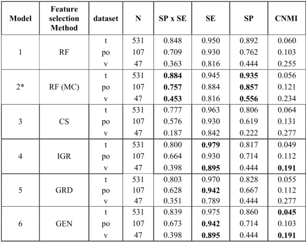
Table 3. The results of C&RT classification analysis using different feature selection

420

methods with equal misclassification costs applied to the C&RT algorithm

421

Model

Feature selection

Method dataset N SP x SE SE SP CNMI

1 RF t 531 0.848 0.950 0.892 0.060 po 107 0.709 0.930 0.762 0.103 v 47 0.363 0.816 0.444 0.255 2* RF (MC) t 531 0.884 0.945 0.935 0.056 po 107 0.757 0.884 0.857 0.121 v 47 0.453 0.816 0.556 0.234 3 CS t 531 0.777 0.963 0.806 0.064 po 107 0.576 0.930 0.619 0.131 v 47 0.187 0.842 0.222 0.277 4 IGR t 531 0.800 0.979 0.817 0.049 po 107 0.664 0.930 0.714 0.112 v 47 0.398 0.895 0.444 0.191 5 GRD t 531 0.803 0.970 0.828 0.055 po 107 0.628 0.942 0.667 0.112 v 47 0.351 0.789 0.444 0.277 6 GEN t 531 0.839 0.975 0.860 0.045 po 107 0.673 0.942 0.714 0.103 v 47 0.398 0.895 0.444 0.191 2 3 4 5 6 7 8 9 10 11 12 13 14 15 16 17 18 19 20 21 22 23 24 25 26 27 28 29 30 31 32 33 34 35 36 37 38 39 40 41 42 43 44 45 46 47 48 49 50 51 52 53 54 55 56 57 58

7 C&RT

t 531 0.784 0.959 0.817 0.066

po 105 0.694 0.942 0.737 0.095

v 47 0.281 0.842 0.333 0.255

SE= Sensitivity, SP = Specificity; SP × SE = accuracy; CNMI = Cost normalised misclassification index, * misclassification

422

costs applied to feature selection method

423

Comparing models built with equal misclassification costs (Table 3); the best overall model

424

to choose would be model 2. This model has the highest SP x SE, plus the highest specificity 425

values for the training, parameter optimisation and validation sets. However, this model does 426

not achieve the highest sensitivity values, with SE = 0.945, 0.884 and 0.816 for the training, 427

parameter optimisation and validation set respectively. All other models have better SE than 428

model 2 for the three data subsets; apart from model 1, which has the same SE for the 429

validation set, and model 5 (GRD), with a lower SE of 0.789. If the aim of the model was to 430

achieve the best sensitivity then model 6, using genetic search feature selection, would be the 431

best model to use as it achieved the best sensitivity for the parameter optimisation and the 432

highest SE for the training set amongst the three selected models above, along with the lowest 433

CNMI for the training set. Model 2 was able to classify correctly all the permanent 434

ammonium-containing compounds used in the training and parameter optimisation set, and 435

this reflected in the correct prediction of a permanent ammonium containing compounds in 436

the validation set. The classification tree using the molecular descriptors from this model is 437 shown in Figure 3. 438 2 3 4 5 6 7 8 9 10 11 12 13 14 15 16 17 18 19 20 21 22 23 24 25 26 27 28 29 30 31 32 33 34 35 36 37 38 39 40 41 42 43 44 45 46 47 48 49 50 51 52 53 54 55 56 57 58

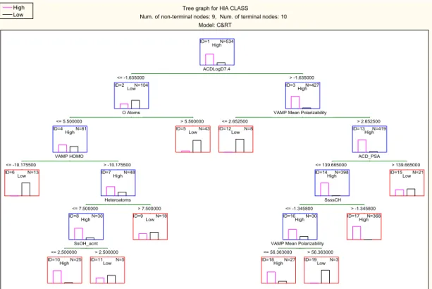
439

Figure 3. Tree graph for C&RT analysis using random forest predictor importance as feature 440

selection method with equal misclassification costs applied to pre-processing C&RT (Model 441

2 in Table 3) 442

Table 4. The results of C&RT classification analysis using different feature selection

443

methods with higher misclassification costs applied to false positives to the C&RT

444

algorithm (misclassification cost ratio of FP: FN = 4:1)

445 Model Feature selection Method dataset N SP x SE SE SP CNMI 8 RF t 531 0.887 0.927 0.957 0.026 po 107 0.725 0.895 0.810 0.068 v 47 0.675 0.868 0.778 0.081 9* RF (MC) t 531 0.879 0.909 0.968 0.028 po 107 0.738 0.860 0.857 0.066 v 47 0.635 0.816 0.778 0.093 10 CS t 531 0.838 0.906 0.925 0.037 po 107 0.687 0.849 0.810 0.079 v 47 0.544 0.816 0.667 0.118 11 IGR t 531 0.853 0.934 0.914 0.033 po 107 0.673 0.884 0.762 0.082

Tree graph for HIA CLASS

Num. of non-terminal nodes: 9, Num. of terminal nodes: 10 Model: C&RT ID=1 N=534 High ID=2 N=104 Low ID=4 N=61 High ID=7 N=48 High ID=8 N=30 High ID=3 N=427 High ID=13 N=419 High ID=14 N=398 High ID=16 N=30 High ID=6 N=13 Low ID=10 N=25

High ID=11Low N=5

ID=9 N=18 Low

ID=5 N=43

Low ID=12Low N=8

ID=18 N=27

High ID=19Low N=3

ID=17 N=368 High ID=15 N=21 Low ACDLogD7.4 <= -1.635000 > -1.635000 O Atoms <= 5.500000 > 5.500000 VAMP HOMO <= -10.175500 > -10.175500 Heteroatoms <= 7.500000 > 7.500000 SsOH_acnt <= 2.500000 > 2.500000

VAMP Mean Polarizability

<= 2.652500 > 2.652500

ACD_PSA

<= 139.665000 > 139.665000

SsssCH <= -1.345800 > -1.345800

VAMP Mean Polarizability <= 56.363000 > 56.363000 High Low 2 3 4 5 6 7 8 9 10 11 12 13 14 15 16 17 18 19 20 21 22 23 24 25 26 27 28 29 30 31 32 33 34 35 36 37 38 39 40 41 42 43 44 45 46 47 48 49 50 51 52 53 54 55 56 57 58

v 47 0.544 0.816 0.667 0.118 12 GRD t 528 0.892 0.943 0.946 0.025 po 106 0.654 0.872 0.750 0.085 v 47 0.725 0.816 0.889 0.068 13 GEN t 531 0.885 0.895 0.989 0.027 po 107 0.640 0.895 0.714 0.090 v 47 0.614 0.789 0.778 0.099 14 C&RT t 531 0.911 0.932 0.978 0.020 po 107 0.726 0.907 0.800 0.066 v 47 0.544 0.816 0.667 0.118

FP = False positive; FN = False negative; SE= Sensitivity, SP = Specificity; SP × SE = accuracy; CNMI = Cost normalised

446

misclassification index, * misclassification costs applied to feature selection method

447

For Table 4, based on the SP x SE for the external validation set the best model is model 12 448

with a SP x SE value of 0.725 but this model also had one of the lowest SP x SE for the po 449

set (0.654) which has a higher number of chemicals compared to the external validation set. 450

In comparison, models 8 and 9 achieved higher SP x SE of 0.725 and 0.738 respectively, 451

where the po set was not used for molecular descriptor selection and hence it was also an 452

external set. From models 8 and 9, model 9 had a similar balance of high estimation of SP 453

and SE compared to model 8 which was slightly worse at predicting poorly-absorbed 454

compounds for the po set. What was interesting to note about model 9 was the feature 455

selection method using predictor importance from random forest, which allowed 456

misclassification costs to be applied at the feature selection level. Then the resulting C&RT 457

model (with misclassification costs) achieved high prediction accuracy for the unseen 458

validation set as well as training and parameter optimisation sets. The C&RT tree for model 9 459 is shown in Figure 4. 460 2 3 4 5 6 7 8 9 10 11 12 13 14 15 16 17 18 19 20 21 22 23 24 25 26 27 28 29 30 31 32 33 34 35 36 37 38 39 40 41 42 43 44 45 46 47 48 49 50 51 52 53 54 55 56 57 58

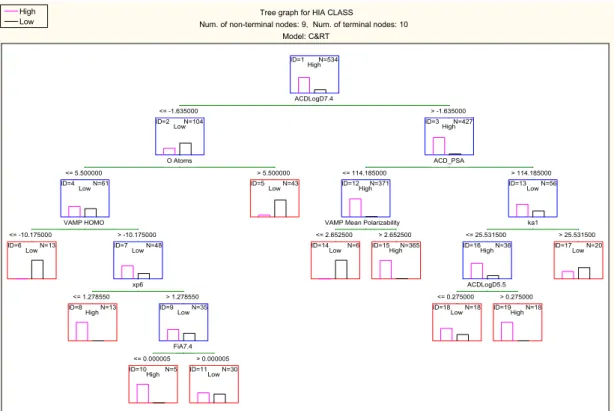
461

Figure 4. Tree graph for C&RT analysis using random forest predictor importance as feature 462

selection method with higher misclassification costs applied to reduce false positives (model 463

9 in Table 4) 464

3.1 Interpretation of the selected models (models 2 and 9)

465

Both models 2 and 9 have been developed using the 20 most significant molecular descriptors 466

selected by random forest analysis. Although the top 20 molecular descriptors were given as 467

input to the C&RT analysis, not all of the molecular descriptors were used to build the 468

decision trees. The first split variable in both models is ACDLogD7.4, the logarithm of the 469

apparent distribution coefficient between octanol and water, and a measure of hydrophobicity 470

at pH 7.4. This molecular descriptor along with logP is used in numerous publications for 471

oral absorption modelling, and has been found to have a positive effect for transcellular 472

absorption 43, 44. For compounds to be split into the high absorption class, LogD7.4 has to be

473

greater than -1.63 according to both models. For compounds with low logD7.4 (≤-1.63), if 474

they contain more than five oxygen atoms they are classed as poorly-absorbed in this terminal 475

node according to both models. This molecular descriptor is linked to the number of 476

hydrogen bond acceptors, highlighted in Lipinski’s rule of five 45_{; which states that a}

477

molecule will be highly likely to be poorly-absorbed if two or more of the following rules are 478

Tree graph for HIA CLASS

Num. of non-terminal nodes: 9, Num. of terminal nodes: 10 Model: C&RT ID=1 N=534 High ID=2 N=104 Low ID=4 N=61 Low ID=7 N=48 Low ID=9 N=35 Low ID=3 N=427 High ID=12 N=371

High ID=13LowN=56

ID=16 N=36 High ID=6 N=13 Low ID=8 N=13 High ID=10 N=5

High ID=11LowN=30

ID=5 N=43 Low

ID=14 N=6

Low ID=15HighN=365

ID=18 N=18

Low ID=19HighN=18

ID=17 N=20 Low ACDLogD7.4 <= -1.635000 > -1.635000 O Atoms <= 5.500000 > 5.500000 VAMP HOMO <= -10.175000 > -10.175000 xp6 <= 1.278550 > 1.278550 FiA7.4 <= 0.000005 > 0.000005 ACD_PSA <= 114.185000 > 114.185000

VAMP Mean Polarizability <= 2.652500 > 2.652500 ka1 <= 25.531500 > 25.531500 ACDLogD5.5 <= 0.275000 > 0.275000 High Low 2 3 4 5 6 7 8 9 10 11 12 13 14 15 16 17 18 19 20 21 22 23 24 25 26 27 28 29 30 31 32 33 34 35 36 37 38 39 40 41 42 43 44 45 46 47 48 49 50 51 52 53 54 55 56 57 58

broken: if molecular weight >500 Da, sum of OH and NH hydrogen bond donors >5, 479

calculated logP (C LogP) >5 and sum of N and O atoms as hydrogen bond acceptors >10. 480

Examples of poorly-absorbed compounds classed in this node are ceftriaxone and raffinose. 481

In both models, the next important descriptor selected for the partitioning of compounds with 482

low logD7.4 and less than six oxygen atoms is VAMP HOMO. This molecular descriptor is 483

the energy of the highest occupied molecular orbital calculated by AM1 semi-empirical 484

method using the VAMP programme in TSAR 3D software. The higher the value (>-10.18 in 485

the split in the trees) indicates higher absorption classification. Compounds with low HOMO 486

values are in the low absorption terminal nodes; and correlates with previous research 28. The

487

majority of compounds with low HOMO energy (<-10.18) according to this split contain a 488

permanent quaternary ion such as pralidoxime and bethanechol, which are small polar 489

molecules mainly related to the neurotransmitter acetylcholine, or compounds such as 490

fosmidomycin and fosfomycin, which contain phosphorus atoms. Compounds with a higher 491

HOMO energy are further split with different molecular descriptors in the two trees. 492

In Figure 3 compounds with more than seven heteroatoms are classed as poorly-absorbed. 493

This corresponds to Lipinski’s rule of five, more precisely the number of hydrogen bond 494

acceptors rule. In this node the majority of compounds are antibiotics such as meropenem and 495

imipenem, which are both poorly-absorbed. There are also some misclassified antibiotics 496

such as penicillin V and amoxicillin, which are highly-absorbed. However, both these 497

compounds have been found to be substrates for the oligopeptide transporter, PEPT1 498

(SLC15A1), influx transporter in the small intestine 46_{. The remaining 30 compounds are}

499

classed as highly-absorbed if they contain less than three OH groups (SsOH_Acnt). 500

In Figure 4 however, compounds with low xp6 values are classed as highly-absorbed. The 501

descriptor xp6 is the sixth order single path molecular connectivity index 9, which may be

502

regarded as a size descriptor with some shape/connectivity elements. Examples of 503

compounds in this node are of a small, polar often peptide like nature with no permanent 504

charge and mainly natural or semi-synthetic compounds such as phenylalanine and captopril 505

which may have the possibility to be absorbed using oligopeptide transporters (Figure 4,

506

Node ID=8). The remaining 35 compounds are classed as poorly-absorbed if they have 507

acidic groups with ionization fraction > 0.000005. 508

Highly-absorbed compounds with logD value greater than -1.63 are split differently in 509

Figures 3 and 4. Despite this, the best molecular descriptors for splitting of these 427 510 2 3 4 5 6 7 8 9 10 11 12 13 14 15 16 17 18 19 20 21 22 23 24 25 26 27 28 29 30 31 32 33 34 35 36 37 38 39 40 41 42 43 44 45 46 47 48 49 50 51 52 53 54 55 56 57 58

compounds in both trees are the same, namely polarizability (VAMP mean polarizability) and 511

polar surface area (ACD_PSA). In both trees, compounds with polarizability values ≤ 2.65 512

are poorly-absorbed. This molecular descriptor indicates the distortion of a compound’s 513

electron cloud by an external electric field 47. Examples of compounds with ≤2.65

514

polarizability values (Node ID = 12 in Figure 3 and 14 in Figure 4) are bephenium and

515

vecuronium, both with low polarizability due to the permanent quaternary ion present in the 516

molecules. Polar surface area (PSA) is a common molecular descriptor used in oral 517

absorption models 20, 28. PSA is the area of the Van der Waals surface that arises from oxygen

518

and nitrogen atoms or hydrogen atoms bound to these atoms. In both trees compounds with 519

high PSA are poorly-absorbed. In Figure 3 a compound is poorly-absorbed if the PSA is

520

greater than 139.67Å, which matches the literature threshold value where it was cited that a 521

molecule will be poorly-absorbed (<10% FA) if the PSA is ≥140Å 43, 48_{. In Figure 4, a}

522

threshold value of 114.19 Da has been used but these high PSA compounds have been 523

partitioned further and those with smaller molecular size as indicated by ka1, and higher 524

logD5.5 values than 0.275 are classed as highly-absorbed. An interesting feature can be 525

observed in Figure 3, where for the compounds with PSA values ≤139.67 and low index for

526

>CH- groups (SsssCH ≤ -1.35), if polarizability is too high (VAMP mean polarizability 527

>56.363) then oral absorption will be poor. Examples of these drugs are two pro-drug ACE 528

inhibitors moexipril diacid and fosinopril plus the cardiac glycoside cymarin. 529

3.2 Chemical space and repeating misclassifications in models

530

There were a few compounds that were continually misclassified by most models. Within the 531

validation set the compounds misclassified by all models was lovastatin, while frovatriptan 532

was misclassified by the majority of models. These compounds are poorly-absorbed, but the 533

models misclassified them as highly-absorbed. Lovastatin is a naturally occurring product 534

used to reduce cholesterol; this compound has poor solubility issues in aqueous medium 49,

535

plus it has been identified as heavily undergoing gut metabolism both of which could account 536

for the misclassification 50. In addition, this compound has been identified as a potential

537

substrate and inhibitor of the efflux transporter P-gp 51. Frovatriptan, according to the Varma

538

et al (2010), has a fraction escaping gut metabolism of 69% meaning potentially, 30% could 539

be metabolised by the gut, specifically UDP-glucuronosyltransferases (UGT’s) in the gut due

540

to their substrate specificity of the indole group present in frovatriptan and the similarity of 541

this compound to serotonin, a UGT substrate. However there is no direct evidence of this in 542

the literature however this could explain the misclassification by our models 52, 53.

543 2 3 4 5 6 7 8 9 10 11 12 13 14 15 16 17 18 19 20 21 22 23 24 25 26 27 28 29 30 31 32 33 34 35 36 37 38 39 40 41 42 43 44 45 46 47 48 49 50 51 52 53 54 55 56 57 58

4. Discussion

544

Thousands of molecular descriptors can be calculated to represent molecular features or 545

properties of the compounds. The use of feature selection to reduce the number of molecular 546

descriptors is a common practice in QSAR as a part of pre-processing or embedded methods. 547

Feature selection increases interpretability by reducing the number of molecular descriptors, 548

it reduces overfitting associated with noisy or redundant descriptors and often improves 549

predictability of resulting classification models. 550

In this paper we used various filter feature selection methods for data pre-processing, to pick 551

significant descriptors related to intestinal absorption. These descriptor sets were used as 552

input for C&RT analysis, which has an embedded feature selection method, to classify 553

compounds into high or low absorption in a biased dataset. The application of higher 554

misclassification costs for false positives to the C&RT analysis was also investigated to 555

overcome the problem of biased datasets (which contain many more highly-absorbed 556

compounds than poorly-absorbed compounds) and to see if models with greater prediction 557

accuracy could be achieved. 558

The feature selection methods used in this work were predictor importance using random 559

forest (RF), chi square (CS), information gain ratio (IGR), greedy search (GRD) and genetic 560

search (GEN). The feature selection methods were compared based on the predicted ability of 561

the C&RT algorithm. There were certain expectations of the feature selection methods based 562

on how they work and their advantages and disadvantages. To begin, it was expected that the 563

combination of a pre-processing feature selection method and C&RT, which has an 564

embedded feature selection, to have higher prediction accuracy when compared to using 565

C&RT with no pre-processing feature selection method. This was on the basis that when 566

C&RT splits compounds, further down the tree there are fewer compounds in the deeper 567

nodes, therefore less statistical support for an effective selection of the best descriptor 568

especially when there are a larger number of molecular descriptors to choose from. Therefore 569

as a result the C&RT algorithm could pick descriptors that may be less relevant to molecular 570

descriptors higher up in the tree. However, C&RT is a successful technique in its own right 571

with an embedded feature selection function which is used in model development for the 572

prediction of oral absorption 28, 54. The benefits of using C&RT are that it can cope with noisy

573

data (to some extent) of moderately sized biased datasets 11 and produces models (decision

574 2 3 4 5 6 7 8 9 10 11 12 13 14 15 16 17 18 19 20 21 22 23 24 25 26 27 28 29 30 31 32 33 34 35 36 37 38 39 40 41 42 43 44 45 46 47 48 49 50 51 52 53 54 55 56 57 58

trees) that in principle can be easily interpreted. In addition it is less time consuming than 575

pre-processing the molecular descriptors first. 576

The expectations of the feature selection methods themselves can be considered and 577

compared to the obtained results in this work. The benefits of simple univariate filter 578

techniques such as CS and IGR are that they are simple and fast to compute; however they 579

fail to take into account molecular descriptor interactions 18, 55. This is in contrast to GRD and

580

GEN, which take molecular descriptor interactions into account but are more computationally 581

expensive. In a comparison of GRD and GEN, due to the way these feature selection methods 582

work, GEN should achieve higher accuracy, as it performs a global search in the molecular 583

descriptor space, whilst GRD performs a local search in the molecular descriptor space. 584

Using the predictor importance in the random forest method is computationally expensive; 585

however, there is the added advantage that misclassification costs can be applied using the 586

software as well as being applied for the C&RT analysis. Finally, based on previous research, 587

the application of higher misclassification costs to false positives will produce models with 588

increased overall accuracy and reduced false positive misclassifications, therefore 589

overcoming the problem of biased datasets compared with equal misclassification costs. 590

Overall, one of the best feature selection methods according to the models produced in this 591

work was predictor importance using random forest. This was expected for this method, as it 592

was possible to apply higher misclassification costs to the feature selection technique itself as 593

well as applied to the C&RT analysis. Even when misclassification costs were not applied to 594

predictor importance, the produced models still had higher overall accuracies over most 595

models. This is down to the ensemble nature of this method, which is known to perform 596

better than single tree analysis 56. In comparison with C&RT where no pre-processing feature

597

selection was utilised, the predictor importance feature selection method had higher overall 598

accuracy for the validation set in all cases. The high classification accuracy on the training set 599

but low prediction accuracy on the validation set could indicate overfitting of the models 600

produced by C&RT. Models produced by other pre-processing feature selection techniques 601

were better compared with models produced by C&RT with no pre-processing feature 602

selection on the validation set, except for the models produced by CS feature selection. In the 603

majority of the cases, using C&RT alone gave better prediction accuracy for the parameter 604

optimisation set compared with IGR, GRD and GEN; however these latter methods had better 605

overall prediction accuracy for the validation set. This shows that C&RT without pre-606

processing can cope with redundant and meaningless molecular descriptors, however is prone 607 2 3 4 5 6 7 8 9 10 11 12 13 14 15 16 17 18 19 20 21 22 23 24 25 26 27 28 29 30 31 32 33 34 35 36 37 38 39 40 41 42 43 44 45 46 47 48 49 50 51 52 53 54 55 56 57 58

to overfitting (even with pruning of the trees) and can lack predictive accuracy for the 608

prediction of the validation set. 609

Comparing the expectations set out initially, it was found that comparing univariate methods 610

such as CS and IGR with those that take into account molecular descriptor interactions (GEN 611

and GRD) there is no clear pattern in the difference between their results. However, overall, 612

when equal misclassification costs were applied to the C&RT analysis, GEN as expected had 613

better or comparable predictor performance than CS and IGR. On the other hand, GRD had 614

comparable performance with CS and weaker compared with IGR. When misclassification 615

costs were applied to C&RT, GEN and GRD models were better than CS and IGR for the 616

training and validation set, again it is difficult to state which method is better overall. This 617

effect is also seen in the next example when comparing GEN and GRD feature selection 618

methods based on the predictive accuracy of the C&RT analysis. GEN performs better than 619

GRD when equal misclassification costs were used; this matches the predictions previously 620

made. This is in some agreement with work using numerical regression analysis 57. However

621

upon applying higher misclassification costs the molecular descriptors pre-processed by the 622

GRD model outperformed the GEN model. This could be due to the correlation-based feature 623

selection subset evaluator used by the GEN method not being suitable for use with C&RT 624

and misclassification costs, and potentially highlight overfitting by the GEN based model. 625

The effect of applying higher misclassification costs to either false positives or false 626

negatives has been investigated in previous research 28_{. In this work the application of higher}

627

misclassification costs to false positives resulted in better overall accuracy and specificity as 628

expected in the majority of cases. 629

In this work we have shown that for most models using pre-processing feature selection does 630

appear to improve classification accuracy compared to the control (C&RT using all molecular 631

descriptors) based on prediction accuracy. This agrees with work carried out by Xue and co-632

workers16 _{who considered three different datasets including prediction of oral absorption.}

633

They used recursive feature elimination for feature selection and SVM to classify 634

compounds. They compared the results with and without the feature selection method and 635

found that for oral absorption improved accuracy was obtained when the feature selection 636

method was used. For one of the datasets, feature selection gave comparable predictive 637

ability, which with a smaller descriptor subset will increase the interpretability of resulting 638

models 16. However, a study by Suenderhauf11 carried out regression and classification for

639

oral absorption using a variety of techniques including C&RT, Support Vector Machine 640 2 3 4 5 6 7 8 9 10 11 12 13 14 15 16 17 18 19 20 21 22 23 24 25 26 27 28 29 30 31 32 33 34 35 36 37 38 39 40 41 42 43 44 45 46 47 48 49 50 51 52 53 54 55 56 57 58