New methods for the sensitivity analysis of
black-box functions with an application to
sheet metal forming
A doctoral Thesis
by
Jana Fruth
in fulfillment of the requirements for the degrees “Doktorin der Naturwissenschaften der Technischen Universit¨at Dortmund” and “Docteur de l’´Ecole Nationale Sup´erieure des Mines de Saint-´Etienne”
Submitted to TU Dortmund University and Mines Saint-Etienne
Prof. Dr. Katja Ickstadt Head of the jury Prof. Dr. Sonja Kuhnt Reviewer
Prof. Cl´ementine Prieur Reviewer Prof. Dr. Joachim Kunert Reviewer Prof. Olivier Roustant Supervisor Prof. Rodolphe Le Riche Examiner
Acknowledgements
I deeply thank my supervisors Sonja Kuhnt in Dortmund and Olivier Roustant in Saint-´Etienne for giving me the chance to research on such an interesting topic, to get insight into the research work of two difference places, and to meet so many exciting people. I feel very lucky for that and as well for the great, constant support which I could not have imaged any better.
Furthermore, I want to thank some of the many people that helped me to write this thesis, e.g. by inspiring scientific conversations and inputs, amazing programming support, great cooperations, constant assistance, or kind encouragements: Thomas M¨uhlenst¨adt, Laurent Carraro, Cl´ement Chevalier, David Ginsbourger, Bertrand Iooss, Roland Jegou, Art B. Owen, Cl´ementine Prieur, Marc Roelens, David Steinberg, Mom-chil Ivanov, Hamad ul Hassan, Andr´e K¨onig, Uwe Ligges, Olaf Mersmann, Daniel Vogel, Stefan Hess, Simon Neum¨arker, Malte Jastrow, Matthias Borowski, Thoralf Mildenberger, Andr´e Rehage, Nikolaus Rudak, Henrike Weinert, Ieva Zelo, and Jakob Wieczorek.
Last but not least, I want to thank the Deutsche Forschungsgesellschaft for funding via SFB 708 project C3.
Contents
1 Introduction 1
2 Sensitivity Analysis 5
2.1 Background . . . 5
2.2 The role of metamodels . . . 6
2.3 Variance-based indices . . . 8
2.3.1 Definition of various variance-based indices . . . 10
2.3.2 Monte Carlo estimation . . . 12
2.3.3 Frequency-based estimation . . . 17
2.4 Derivative-based methods . . . 20
2.4.1 Morris screening by elementary effects . . . 20
2.4.2 DGSM . . . 21
2.5 Ongoing developments in sensitivity analysis . . . 23
3 Sensitivity Analysis for Interaction Screening 25 3.1 Total interaction indices . . . 28
3.2 TII estimation . . . 31
3.3 Theoretical properties of TII estimators . . . 34
3.4 Estimating the full set of TIIs . . . 41
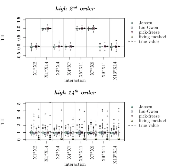
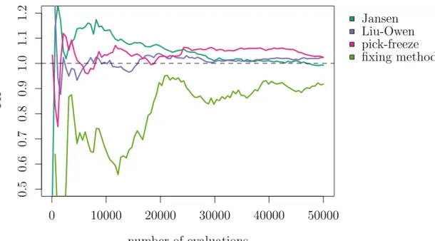
3.5 Simulation study . . . 42 i
3.6 Threshold decision . . . 48
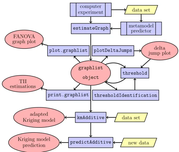
3.7 Implementation . . . 54
3.8 Crossed DGSM . . . 56
4 Sensitivity Analysis for Functional Input 61 4.1 Sequential functional sensitivity analysis . . . 64
4.2 Error-free test cases . . . 70
4.3 Splitting and design . . . 74
4.4 Implementation . . . 77
4.5 Analytical example . . . 77
5 Support Analysis 83 5.1 Support index functions . . . 84
5.2 Analytical example . . . 89
5.3 Expected values . . . 89
6 Application to a Sheet Metal Forming Process 93 6.1 Thickness reduction . . . 95
6.2 Functional input application . . . 103
7 Conclusion and Outlook 109
A Notations 111
B Data 115
Chapter 1
1.
Introduction
This work deals with the topic of sensitivity analysis for computer experiments. In the situation that statistical experiments are too expensive, time-consuming, might harm lives, or are simply impossible to perform, computer simulations can sometimes be used as a replacement. These computer experiments are complex mathematical models constructed from known physical relations, e.g. in engineering or environmen-tal problems, or chemical and medical experiments, where computer experiments are also known as in silico experiments. Specific examples for computer experiments are traffic simulation models (Punzo and Ciuffo, 2011), where the interest lies in observing those effects that lead to congestions, models of manufacturing processes like the deep drawing model which motivated this work, or highly complex weather models, used in the climate impact research (Katz, 2002). Computer experiments have become every-day procedures in those fields and are also rising in other areas like social sciences and economics. None the less, it has to be kept in mind that computer experiments are only approximations of the real process and should be validated by real experiments whenever possible.
From the statistical point of view, computer experiments have to be treated specially since they are usually deterministic, contain a high number of input variables and are highly complex in terms of nonlinear relations and interactions. The inherent mathematical equations are most often solved numerically which results in long-lasting
computations, so computer experiments can be very time-consuming. Methods have been developed for the design of computer experiments, above all space-filling designs like Latin hypercubes, maximin design, or entropy design (Santner et al., 2003). For deterministic modeling and prediction, advanced interpolation methods exist which respect the high complexity, with the most popular being the Gaussian process emula-tor, also called Kriging. Finally, there are also optimization procedures for computer experiments, which make use of the prediction models, one popular method being the Kriging-based EGO algorithm, which utilizes the fact that Kriging provides an estima-tion of the uncertainty of unobserved points.
In this work, the focus lies on a further broad field in the analysis of computer ex-periments, sensitivity analysis, which has importance in all steps beginning with the building of the computer experiment over its use and understanding to model building and model validation. It analyzes how sensitive the computer experiment responds to variations in the input.
The analysis of the response’s sensitivity is of interest on its own, e.g. to answer the question what happens in a car crash simulation when the tire friction changes. Based on Saltelli et al. (2000), five further points of sensitivity analysis application can be named:
(1) To check, if a model resembles the real process, i.e. if sensitivities reflect expec-tations,
(2) to determine the most important input variables and optimal regions in the space of input variables for calibration studies,
(3) to select and rank input variables by importance,
(4) to detect regions in the space of input variables for which the model variation is maximum, and
3
This work presents new sensitivity analysis methods, motivated by and framed around applications in the analysis of shape accuracy in sheet metal forming. Shape defor-mation after the removal of the forming punch is a serious problem in production processes, but can be simulated by finite elements methods (FEM).
With regard to point (5), the total interaction index (TII) for the analysis of computer experiments is presented, an extension to the usual Sobol indices. Defined for two input variables at a time, it gives the sum of Sobol indices of any order interaction containing both input variables. If we estimate the TII for all combinations of the two input variables, we can get an overview of the complete interaction structure of the computer experiment, a difficult task with Sobol indices due to the curse of dimensionality. The structure can be intuitively drawn in a so-called FANOVA graph (M¨uhlenst¨adt et al., 2012). Furthermore, similar to the input variable screening by Sobol indices, we can use TIIs for interaction screening. This leads to a block-additive decomposition of the computer experiment. An inactive interaction indicates that the two input variables come from two groups of variables that have no interaction in common and thus are additive. This knowledge about a block-additive structure in the computer experiment can be applied in subsequent procedures. Metamodels like Kriging can be adapted to follow the block-additive structure and optimization can be simplified and parallelized when being performed in each block separately. We present several estimation methods for the TII and analyze their statistical properties. Methods for interaction screening, including a suitable thresholding algorithm for inactive interactions, are developed. In addition, derivative-based indices, which provide a faster-to-compute upper bound for the TII, are presented.
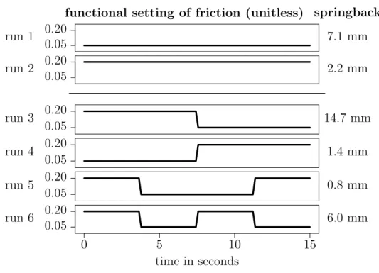
Usually the process parameters are kept on a constant level during the computer exper-iment. For the deep drawing analysis, finite element simulations have been developed that allow the user to change parameters during the forming process in order to further improve the accuracy of the analysis. Here new methods are necessary for the sensi-tivity analysis of those temporal changeable parameters. This work presents an idea
for an effective sensitivity analysis of functional input including design and graphical representation of the functional influences of the inputs. To keep the number of func-tion evaluafunc-tions as low as possible, a sequential algorithm is introduced that increases the accuracy of the functional sensitivity analysis with every step. The points (1), (2) and (3) can be handled by the methods for functional input variables.
The ideas of the sequential algorithm are further developed for the analysis of the support of scalar input variables, the support analysis. Regarding point (4) the aim is to analyze the sensitivity of the different regions of the variables’ distribution support. This information gives closer insight into the impact of the variables in the process and can furthermore help in finding optimal support settings for screening, modeling, and sensitivity analysis. In this work, support index functions as well as visualization methods are suggested and their relations to other indices are derived.
The thesis is structured as follows. Chapter 2 gives an introduction to sensitivity analysis together with a panorama of the current state of research in the field with special focus on variance-based global sensitivity indices. Chapter 3 introduces the TII along with the complete methodology for sensitivity analysis of the interaction structure. Chapter 4 presents the approach of sensitivity analysis for functional input and in Chapter 5 the developed technique for support analysis is presented. All methods are then applied in deep drawing simulations in Chapter 6. The work is concluded with a summary and outlook in Chapter 7.
Chapter 2
2.
Sensitivity Analysis
2.1
Background
In the field of computer experiments, sensitivity analysis generally explores the rela-tionships between information flowing in and out of the experiment. More specifically, it studies how the uncertainty in the output of the computer experiment can be appor-tioned to different sources of uncertainty in the inputs with the direct aim of process understanding and input variable screening, but also calibration, metamodel building and finally optimization. An elaborate overview can be found in the standard work of sensitivity analysis by Saltelli et al. (2000) and in the comparison of sensitivity analysis techniques by Confalonieri et al. (2010). This chapter starts with a brief outline of the background of sensitivity analysis.
In the beginning, sensitivity analysis was based on standard statistical methods like scatter plots. There, the influence of a variable can be read from plots of the output against each input variable. Further methods were regression analysis, where regres-sion coefficients qualify the linear sensitivity of each input (e.g. Kleijnen (1997)) and correlation analysis. A next step were one-at-a-time methods (e.g. Daniel (1973)). Here, one input variable is changed while keeping all other at a constant level, thus information can be obtained only for that particular region in the input space. A sim-ilar approach came from chemical modeling (e.g. Chapter 5 of Saltelli et al. (2000)),
which uses partial derivatives around a nominal value as local sensitivities. In con-trast to those local methods, Schaibly and Shuler (1973) developed a global sensitivity analysis method called FAST (Fourier amplitude sensitivity test), which allows for all input variables to be varied at the same time. Here, the input variables are sampled in such a way that the amplitudes obtained by a Fourier analysis of the output can be interpreted as sensitivity indices of the input variables. Later on, Sobol’ (1993) introduced indices, which are now called Sobol indices, global sensitivity indices, which have been proved by Saltelli and Bolado (1998) to predict the same quantities as the FAST indices. Because of their clear interpretation, unbiased estimation and their access to interactions, Sobol indices have been widely used and are being further de-veloped continuously. Parallel to that, alternative sensitivity analysis methods were introduced like derivative-based indices (Kucherenko et al., 2009) and, based on one-at-a-time methods, very effective screening designs have been developed with the most important being Morris screening (Morris, 1991).
2.2
The role of metamodels
The estimation of sensitivity indices usually requires a high number of model evalu-ations, as crude discrete integration methods are applied. Time-consuming computer experiments are therefore often replaced by a faster-to-evaluate second model, which is called a metamodel, surrogate model, emulator or response surface. Possible meta-models come from the large field of the modeling of computer experiments (e.g. Fang et al., 2006), a popular one being the Gaussian process model described below, but also polynomials, Polynomial Chaos Expansion, splines, or Neural Networks. As the metamodel is only an approximation of the real experiment, a metamodel error has to be taken into account and the accuracy of the model has to be assessed carefully, e.g. by leave-one-out cross validation.
2.2 The role of metamodels 7
Throughout this thesis, there will be no distinction between the true computer exper-iment and the metamodel. The term underlying model, symbolized by f, can either refer to the direct computer experiment or to a metamodel with negligible error. The underlying model f will be regarded as a black-box function, whose specific shape is inaccessible. However, there are some approaches that are able to utilize the specific properties of a metamodel. Blatman and Sudret (2010) compute Sobol indices analyti-cally from Sparse Polynomial Chaos Expansion models and Marrel et al. (2009) define indices for the Gaussian process model that use the Gaussian process directly instead of the prediction function.
The Gaussian process model, also called Kriging as it was proposed by Krige (1951), is a standard tool in computer experiments for various reasons. It interpolates the data, which is important for deterministic computer codes. In addition, the Kriging model performs well in predicting, even for highly complex functions, and it gives a measure of uncertainty at unobserved points (Fang et al., 2006). The basic idea is to assume that the function is a realization of a Gaussian process with a linear trend as mean,
Y(x) = p
X
`=1
β`f`(x) +Z(x), (2.1)
where x = (x1, . . . , xd) represents the vector of d input variables, f1(x), . . . , fp(x) are p known regression functions with β1, . . . , βp the corresponding parameters, and Z(.) is a Gaussian process with zero mean and covariance function, or kernel k. A particular class for the covariance kernel is the stationary family, which implies that k depends only on the difference between two different locations, k(x(1)−x(2)) with k(.) =σ2R(.;θ), where σ2 is the process variance, R the correlation function and θ a vector of covariance parameters.
As the Gaussian process model in (2.1) returns a Gaussian process instead of a function, the predictor has to be defined separately,
b y(x∗) = p X `=1 β`f`(x∗) +k(x∗)0K−1(y−F β), (2.2)
with x∗ a new point at which to predict, K the covariance matrix at all data points,
k(x∗) the covariance vector between the data andx∗, and F the experimental matrix containing the trend values at all data points. Usually, the parameters βk, σ2 and θ are estimated by numerical maximization of the likelihood and inserted into Equation (2.2).
In practice, the kernels are often modeled as tensor products of one-dimensional kernels,
k(h) =σ2 d
Y
`=1
g`(h`;θ`), (2.3)
where popular one-dimensional covariance functions are the Gaussian, g(h;θ) = exp −h 2 2θ2 ,
and the Mat´ern 5/2,
g(h;θ) = 1 + √ 5|h| θ + 5h2 3θ2 ! exp − √ 5|h| θ ! .
An overview of possible covariance functions and their properties can be found in Rasmussen and Williams (2006). In the one-dimensional covariance functions, the parameter to be estimated,θi, controls the covariance in the direction of input variable xi. If all input variables are scaled equally, the estimates of θi can be used as a first impression of the influence of the variables. A high covariance indicates a flat curve and thus a small influence of the variable whereas a low covariance indicates a higher fluctuation and a stronger influence.
2.3
Variance-based indices
The most popular global sensitivity analysis method, the so-called Sobol indices, is based on the variance of the function, decomposed into additive terms. One of the first
2.3 Variance-based indices 9
to mention this decomposition was Hoeffding (1948), who used it to obtain independent random variables to study properties of U-statistics. Efron and Stein (1981) showed the uniqueness of the decomposition and Sobol’ (1993) revisited it in the context of sen-sitivity analysis. A generalization of the decomposition, the so-called high-dimensional model representation (HDMR), was introduced by Rabitz et al. (1999), who aimed at representing functions as a sum of low-dimensional components. Basing on so many (and more) contributors, the decomposition is known under a variety of names. In this work, it will be referred to as functional ANOVA (FANOVA) decomposition as it provides an ANOVA decomposition of the variance of the function.
Let us consider a black-box function Y = f(X), where X = (X1, . . . , Xd)0 is a vector of independent random variables with distribution µ = µ1 ⊗ · · · ⊗µd, and f is a d-dimensional function f : ∆ → R with f(X) ∈ L2(µ), where L2(µ) denotes the space of square-integrable functions with respect to the measure µ. The function can be decomposed into additive terms,
f(X) = f0+ d X i=1 fi(Xi) + X i<j fi,j(Xi, Xj) +· · ·+f1,...,d(X1, . . . , Xd). (2.4) The terms represent first-order effects (fi(Xi)), second-order interactions (fi,j(Xi, Xj)), and all higher combinations of input variables. The decomposition is unique if all terms fI(XI), I ⊂ {1, . . . , d} have zero mean,
E(fI(XI)) = 0, I ⊆ {1, . . . , d} (2.5)
and the conditional expectations fulfill the non-simplification conditions
E(fI(XI)|XJ) = 0, J ⊂I ⊆(1, . . . , d). (2.6) From (2.5) and (2.6), it follows that the terms also have zero correlation,
E(fI(XI)fI0(XI0)) = 0, I 6=I0.
The decomposition can be obtained by recursive integration, f0 = E(f(X)),
fi(Xi) = E(f(X)|Xi)−f0,
fi,j(Xi, Xj) = E(f(X)|Xi, Xj)−fi(Xi)−fj(Xj)−f0,
and so on. By computing the variance of (2.4), an ANOVA-like variance decomposition is obtained, where each part quantifies the impact of the input variables on the response,
D= Var(f(X)) = Var(f0) + d X i=1 Var(fi(Xi)) + X i<j Var(fi,j(Xi, Xj)) +· · ·+ Var(f1,...,d(X1, . . . , Xd)). (2.7)
2.3.1 Definition of various variance-based indices
The variances
DI = Var(fI(XI)) (2.8)
are known as unscaledSobol indices (Sobol’, 1993). The first-order Sobol index (forI ∈ {1, . . . , d}) is widely used as a sensitivity measure for quantifying the influence of first-order effects. WhenI contains more than one input variable, the Sobol index quantifies the pure interaction influence of the variables indexed in I. As the estimation of the interactions of all possible variable combinations is usually laborious, other indices presented in the following have been developed for the assessment of interactions. The Sobol index is often divided by the overall varianceD, leading to the scaled Sobol index SI = Var(fI(XI)) D = DI D. (2.9)
By this division by the overall variance, the index is normalized to fall between 0 and 1 and thus is easier to assess. The same applies for all indices introduced in the following. For the sake of brevity, they will however be introduced in their unscaled versions since the scaling is equal for all methods considered.
2.3 Variance-based indices 11
An important extension of the Sobol index is the total sensitivity index DT
I (Homma and Saltelli, 1996). Defined for a group of input variables XI for any I ⊆ {1, . . . , d}, it describes the influence of the variables including all interactions of any order that contain at least one of them. Thus, the influence on all orders instead of only the first is measured, which makes it more useful for the screening of input variables. The total sensitivity index is defined as the sum of all partial variances that contain at least one of the variables,
DIT = X J∩I6=∅
DJ. (2.10)
Another way to describe the influence of a group of input variables is the closed sensi-tivity index DC
I , see e.g. Sobol’ (1993), DIC =X
J⊆I
DJ = Var (E[f(X)|XI]). (2.11)
In contrast to total indices, interactions with variables not in XI are not included in this index, but all effects, first-order effects as well as interactions, caused by subsets of it. It is equal to the variance of the conditional expectation and is therefore also known under this name (or shorter VCE) in the literature (McKay, 1995). In its first-order version, it matches the Sobol index.
Sobol indices of higher order can be obtained as a sum of closed sensitivity indices of this order and lower,
DI = |I| X M=1 (−1)|I|−M X J⊆I, |J|=M DCJ. (2.12)
The total and the closed sensitivity index are related by
D=DC−I+DIT, (2.13)
where−I denotes the complement of the setI. Through theformula of total variance, this leads to a further representation of the total sensitivity index,
2.3.2 Monte Carlo estimation
As the computer experiments considered here are treated as black-box functions, the different indices cannot be computed directly, but have to be estimated. The most forward way to estimate the indices, that is the expected values resulting from (2.4), is by crude Monte Carlo integration. A high numbern – typically not less than 1 000×d – of random or quasi-random sampled Monte Carlo runs x(1), . . . ,x(n) is drawn from µ, the distribution of X, to approach the integral,
1 n n X k=1 f(x(k))−−−→n→∞ Z f(X)dµ(X) = E(f(X)). (2.14)
The size of the Monte Carlo sample is denoted bynthroughout this work, except when its specific role is of interest. The approximation is unbiased and, following the strong law of large numbers, convergent with probability one (Caflisch, 1998).
To estimate the closed sensitivity indices, and via them through (2.12) the Sobol in-dices, we need a representation of the index that can directly be adapted to Monte Carlo integration. A common way, sometimes called thepick-and-freeze (or justpick-freeze)
formula, is given by Sobol’ (1993),
DCI = E [f(X)f(XI,Z−I)]−f02, (2.15)
where here as well as in the following, Z stands for an independent copy of X. The constant term and overall variance can be obtained by
f0 = E(f(X)) and D= Var(f(X)).
The corresponding Monte Carlo estimate for twon×d-Monte Carlo samplesx and z
drawn fromµ is straightforward. pf b DIC = 1 n n X k=1 f(x(k))f(x(k)I ,z(k)−I)−fb02, (2.16) b f0 = 1 n n X k=1 f(x(k)), (2.17) b D = Var (fd (x)). (2.18)
2.3 Variance-based indices 13
Alternative expressions, which also take the evaluations f(XI,Z−I) into account in the estimation of f0 and D and thus enable greater numerical stability, have been introduced by Monod et al. (2006, p. 86),
f0 = E f(X) +f(XI,Z−I) 2 , * b f0 = 1 n n X k=1 f(x(k)) +f(x(k) I ,z (k) −I) 2 , (2.19) and D= E f(X)2+f(XI,Z−I)2 2 − E f(X) +f(XI,Z−I) 2 2 , * b D= 1 n n X k=1 f(x(k))2+f(x(k) I ,z (k) −I)2 2 − * b f02. (2.20)
One problem of the pick-freeze estimator (2.16) is that its variance gets very large when f2
0 is large in comparison to DCI. Sobol’ (1993) therefore suggests to shift f by an amount close to f0. Another possibility is to avoid the subtraction of f02. In Owen (2013a), two such estimation strategies called Correlation 1 (Mauntz, 2002, Formula 18) and Correlation 2 are compared. They are based on the representations
DIC = E [f(X) (f(XI,Z−I)−f(Z))]
= E [(f(X)−f(ZI,X−I)) (f(XI,U−I)−f(U))],
with U a further independent copy of X. The corresponding estimates, using Monte Carlo samples x,z, andu fromµ, are much more accurate for small closed sensitivity indices. Cor1 b DCI = 1 n n X k=1 f(x(k))f(x(k)I ,z(k)−I)−f(z(k)), Cor2 b DCI = 1 n n X k=1 f(x(k))−f(z(k)I ,x(k)−I) f(x(k)I ,u(k)−I)−f(u(k)). (2.21)
Though they require more — 3 and 4 — vectors of function evaluations in the integral, no additional evaluations are necessary when applying the strategy of simultaneous estimation of all indices by Saltelli (2002), described later in this Section.
index by Sobol indices by variances computation D(overall variance) P J DJ Var(f(X)) E h f(X)2i−f2 0 E f(XI)2+f(XI,Z−I)2 2 −f2 0
DI (Sobol index) DI Var(fI(XI))
|I| P M=1 (−1)|I|−M P J⊆I, |J|=M DC I DC
I (closed sensitivity index)
P J⊆I DJ Var (E[f(X)|XI]) E [f(X)f(XI,Z−I)]−f02, E [f(X) (f(XI,Z−I)−f(Z))], E [(f(X)−f(ZI,X−I)) (f(XI,U−I)−f(U))] DT
I (total sensitivity index)
P J∩I6=∅ DJ E (Var[f(X)|X−I]) D−DIC, 1 2E h (f(X)−f(X−I,ZI))2 i
Table 2.1: Overview of (unscaled) variance-based indices and their computations.
The total sensitivity index can on the one hand be obtained via the pick-freeze formula using the relation between closed and total sensitivity indices (2.13),
DTI =D−D−IC
=D−E [f(X)f(ZI,X−I)] +f02. (2.22)
Another way, sometimes called the Jansen formula, which avoids the outer sum was first mentioned in Sobol’ (1993) and later improved in Jansen (1999),
DTI = 1 2E (f(X)−f(ZI,X−I))2 . (2.23)
The corresponding estimator Jan b DIT = 1 2n n X k=1 f(x(k))−f(z(k)I ,x(k)−I) 2 .
is proved to be more efficient than (2.22) in Sobol’ (2001, Theorem 4). A proof of its asymptotical efficiency will follow in Chapter 3.
An overview of all presented variance-based indices together with their estimation methods can be found in Tab. 2.1.
2.3 Variance-based indices 15
Estimation of a full set of indices
Saltelli (2002) presents a strategy to recycle runs when the full set of all dindices shall be estimated simultaneously, which is usually the case in applications. They exploit the fact that the two input data setsxand z can be used in more than one way in the estimation of an index. For instance the two pick-freeze formulas
1 n
n
X
k=1
f(x(k))f(x(k)i,j,z(k)−{i,j})−fb02 and
1 n n X k=1 f(zi(k),x(k)−i)f(xj(k),z(k)−j)−fb02
are both estimators for DC
i,j, as they both freeze the variables corresponding to{i, j}. Only the names are changed from xi and xj in the first formula to zi and xj in the second one. Saltelli (2002) shows in his Theorem 1 that, using n(d+ 2) evaluations f(x), f(z), f(x1,z−1), . . . , f(xd,z−d), it is possible to compute
a) each first-order Sobol indexDbi = n1
Pn k=1f(x(k))f(x (k) i ,z (k) −i)−fb02,
b) each total sensitivity index DbiT =Db− n1
Pn k=1f(z (k))f(x(k) i ,z (k) −i) +fb02,
c) each (d−2)-order closed effectDbC−{i,j} = n1
Pn k=1f(x (k) i ,z (k) −i)f(x (k) j ,z (k) −j)−fb02. Dand f2
0 can be estimated from the evaluations as well, e.g. by (2.19) and (2.20). The method further allows for the estimation of all second-order total sensitivity indices and all the corresponding scaled indices.
If in additionn×dmore evaluations f(z1,x−1), . . . , f(zd,x−d) are available, it is possi-ble to obtain second-order closed sensitivity indices as well as doupossi-ble estimates, which allow for more efficient estimation by taking the mean of both estimates. More pre-cisely, we can compute
a) an additional estimate of each first-order Sobol index
b Di = n1 Pn k=1f(z (k))f(z(k) i ,x (k) −i)−fb02,
b) an additional estimate of each total sensitivity index
b DTi =Db − 1n Pn k=1f(x (k))f(z(k) i ,x (k) −i) +fb02,
c) an additional estimate of each (d−2)-order closed effect
b DC−{i,j} = n1 Pn k=1f(z (k) i ,x (k) −i)f(z (k) j ,x (k) −j)−fb02,
d) double estimates of each second-order closed effect b Di,jC = n1 Pn k=1f(x (k) i ,z (k) −i)f(z (k) j ,x (k) −j)−fb02 and b Di,j∗C = n1 Pn k=1f(z (k) i ,x (k) −i)f(x (k) j ,z (k) −j)−fb02,
which further allows again for the estimation of all scaled indices, second-order total sensitivity indices and second-order Sobol indices. Although not mentioned there, it is obvious that the same applies for the total indices estimated by the Jansen formula instead of pick-freeze, which needs the same function evaluations.
Properties of Monte Carlo estimators
To assess the error coming from the Monte Carlo estimation, a straightforward idea is to use bootstrap (Archer et al., 1997). To do this, in the Monte Carlo estimation of an index of interest, thensummands in formula (2.14) are resampled with replacement for a high number of times (≈ 10 000). Each time, the corresponding index is computed and confidence intervals can be constructed from the resulting bootstrap sample. No new evaluations off are necessary, as only the already present evaluations are used. On the other hand, some theoretical results are sometimes available. Janon et al. (2013) discover asymptotic properties of two estimators for the closed sensitivity index (2.11) scaled by the overall variance, DCI
D . Both estimators use formula (2.16) for the estimation, but f0 and the overall variance D are estimated differently. The first estimator, Sbn1, uses the straightforward expressions fb0 (2.17) and Db (2.18),
b Sn1 = 1 n n P k=1 f(x(k))f(x(k) I ,z (k) −I)− 1 n n P k=1 f(x(k)) 2 1 n n P k=1 f(x(k))2− 1 n n P k=1 f(x(k)) 2 , (2.24)
2.3 Variance-based indices 17
whereas in the second, Sbn2, the more stable estimators
* b f0 (2.19) and * b D (2.20) are applied, b Sn2 = 1 n n P k=1 f x(k) fx(k)I ,z(k)−I− 1 n n P k=1 f(x(k))+fx(k) I ,z (k) −I 2 2 1 n n P k=1 f(x(k))2+fx(k) I ,z (k) −I 2 2 − 1 n n P k=1 f(x(k))+fx(k) I ,z (k) −I 2 2 . (2.25)
Janon et al. (2013) show that both estimators are consistent,
b Sn1 −→a.s. n→∞ DC I D , Sb 2 n a.s. −→ n→∞ DC I D ,
and that they are asymptotically normal in the form of √ n b Sn1− D C I D d −→ n→∞ N 0, σ 2 1 , √n b Sn2− D C I D d −→ n→∞ N 0, σ 2 2 .
See Janon et al. (2013, Prop. 3.3) for the specification of the variances σ2
1 and σ22. In their main result, they show that Sbn2 is asymptotically efficient for the estimation of
DC
I/D in the notion of van der Vaart (1998, Chapter 25) in a framework with
exchange-able variexchange-ables.
2.3.3 Frequency-based estimation
Beside direct Monte Carlo estimation, there is a further class of estimation methods, the frequency-based estimation, which is computationally cheaper than Monte Carlo estimation, but also slightly biased.
The first method introduced is the Fourier amplitude sensitivity test (FAST) by Cukier et al. (1978), which allows for the estimation of first-order Sobol indices. Sample points of X are chosen such that the indices can be interpreted as amplitudes obtained by Fourier analysis of the function. More precisely, the design ofnFASTpoints is such that
x(k)i =Gi(sin(ωisk)), i= 1, . . . , d, k = 1, . . . , nFAST, sk= 2π(k−1) nFAST
with Gi functions to ensure that the sample points follow the distribution of X. The set of integer frequencies {ω1, . . . , ωd}, associated to the input variables, is chosen to be as free of interferences as possible, where free of interferences up to the order M means thatPp
i=1aiωi 6= 0 for
Pp
i=1|ai| ≤M+ 1 (Tissot and Prieur, 2012). In practice M = 4 orM = 6 are used.
For a weightω, the Fourier coefficients for each input variable can then be numerically estimated by b Aω = 1 nFAST nFAST X j=1 f(x(sj)) cos(ωsj), b Bω = 1 nFAST nFAST X j=1 f(x(sj)) sin(ωsj), (2.26)
and the first-order Sobol indices can be estimated by the sum of the corresponding amplitudes up to the orderM,
FAST b Di = 2 M X p=1 (Ab2pω i+Bb 2 pωi). (2.27)
An estimate of the overall variance is given by the sum of all amplitudes, FAST b D= 2 nFAST/2 X n=1 (Ab2n+Bbn2). (2.28)
Extended FAST (EFAST), first presented in Saltelli et al. (1999), is a method to also compute total sensitivity indices for single input variables using FAST. Here, a high frequencyωiis assigned to the variable in questionXiand low frequencies, e.g. ω−i = 1, are assigned to all other variables. Then the total sensitivity index of Xi is estimated over the amplitude for the low frequencies,
EFAST b DTi =D−2 M X p=1 (Ab2pω −i+Bb 2 pω−i).
2.3 Variance-based indices 19
A similar method, which avoids the problem of interferences, is RBD-FAST, where the RBD stands for random balanced design. RBD-FAST is a group of modifications of FAST, which use random permutations of design points to avoid interferences. The original idea by Tarantola et al. (2006) is to assign the same frequency to all input variables, but to randomize their values independently before evaluating f. The first-order Sobol index ofXi can then be estimated by reordering the evaluations in the way Xi was permuted, so that the amplitude at the frequency returns the sensitivity of Xi only. This works because the order of the evaluations is important in (2.26). Thus, all first-order Sobol indices can be estimated simultaneously with one set of evaluations. In the same work a further RBD-FAST method called Hybrid is mentioned by which second-order and second-order closed sensitivity indices can be estimated.
Mara (2009) suggests a RBD-FAST method to compute the total sensitivity index of a group of variables DbTI. Here, simple frequencies like ω ={1, . . . , d} are assigned to
the variables. Then nRBD = 2(M d+L) design points are generated over a periodic curve, with L > 100 a tunable integer number, which regulates the sample size. The values of all variables in I are then randomly permuted, either differently per variable or identically, and the experiment is evaluated at the points. The total sensitivity index is estimated by RBD b DTI = nRBD L nRBD/2 X p=dM+1 (Ab2p+Bbp2). (2.29)
The EASI algorithm by Plischke (2010) is a further frequency-based method for the estimation of first-order Sobol indices. It has the advantage that no specific sampling scheme is necessary, which makes it possible to use already available data. It can be seen as a reverse RBD-FAST approach. The evaluations are reordered so that the xi are approximately triangular-shaped, which corresponds to the frequencyω= 1. Then the first-order Sobol index can be estimated as for RBD-FAST.
2.4
Derivative-based methods
This section shows different sensitivity analysis methods that, in contrast to variance-based methods, use the partial derivative of an input variable as an indicator of its influence. As the derivative quantifies the change in the output when the variable is changed, it can be used as a sensitivity measure.
2.4.1 Morris screening by elementary effects
In the field of input variable screening in computer experiments, that is finding the important variables out of a large number of variables using a minimal number of runs, Morris screening is one of the most popular methods (Morris, 1991). Among the advantages of the method over common screening methods are that it covers the entire input space and that it is not restricted to linear influences. Partial differences at different points in the input space, so-called elementary effects, are computed
di(x) =
|y(x1, . . . , xi + ∆p, . . . , xk)−y(x)| ∆p
,
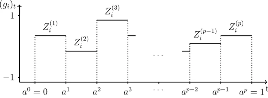
where the values of x are sampled on a grid with p levels for each input and ∆p is a predetermined multiple of 1/(p−1). The distribution of the di provides information on the behavior of Xi. The mean, the so-called Morris Importance Measure, indicates the overall influence. The standard deviation indicates the linearity of the influence. A value close to 0 suggests linear behavior, a high value nonlinear or interaction behavior. To obtain the distribution of elementary effects, the values ofxare sampled randomly or by a more elaborate design that uses trajectories in the space of the input variables, starting from random points on the grid. This reduces the number of necessary runs almost by half compared to random sampling, resulting in a total number of r(d+ 1) runs, with r the number of elementary effects per variable.
2.4 Derivative-based methods 21
2.4.2 DGSM
A more accurate method based on Monte Carlo integration was introduced by Kucherenko et al. (2009). They use indices they call derivate-based global sensitivity measures (DGSM), first presented by Sobol’ and Gershman (1995) as an interpretation of variance-based indices. In contrast to Morris screening, the square of the partial derivative is used, νi = Z ∂f(X) ∂Xi 2 dµ(X). (2.30)
Like variance-based indices, the DGSM quantify the influence of the input variables and they share with the total sensitivity indices the ability that, (under the mild assumption thatµis continuous and its support is equal to the domain ∆ ofX), ifνi = 0, thenf(x) does not depend on xi. Indeed, Sobol’ and Kucherenko (2009) could show a connection between the two sensitivity methods for the uniform and normal distributions, which was extended by Lamboni et al. (2013) for general continuous distributions. It states that
DiT≤ C(µi)νi, (2.31)
provided that µ belongs to a class of distributions that satisfy a Poincar´e inequality,
Z
g(X)2dµ(X)≤C(µ)
Z
k∇g(X)k2dµ(X), (2.32)
for all functions g in L2(µ) such that R
g(X)dµ(X) = 0, and k∇gk ∈ L2(µ). A
Poincar´e constant C(.) is a characteristic of the corresponding distributionµ. The best possible constant for a given distribution, the optimal Poincar´e constant, is denoted by Copt(µ). When C(µ) =Copt(µ), there can exist certain functions fopt for which the Poincar´e inequality is an equality. See Lamboni et al. (2013) or Roustant et al. (2014) for a comprehensive summary.
Formula (2.31) implies that the DGSM can be used as upper boundaries for the total sensitivity indices and thus can serve as a cheaper method for the screening of non-influential input variables since, after Lamboni et al. (2013), the DGSM seems to be
computationally more tractable than variance-based measures, especially for problems with higher numbers of inputs. This applies especially when the computer experiment additionally provides the partial derivatives. Then, the Monte Carlo integration can be performed directly. If not, the derivatives can be approximated numerically by finite differences. The DGSM for a n×d data set x and a small real number δ∗ can be estimated by b νi = 1 n n X k=1 f(x(k)i +δ∗,x(k)−{i})−f(x(k)) δ∗ !2 .
To explore the difference between the DGSM and variance-based indices, let us compare two one-dimensional case functions,
f1(x) = 1 1 + 49 exp(−2 log(49)x), f2(x) = 1 2sin(50x) + 1 2. (2.33)
Plots are shown in Fig. 2.1. In this one-dimensional situation, the total index, the main index, and the overall variance coincide, the variance-based index reduces to
D1 =DT1 =D= 1 Z 0 f(x)2dx− 1 Z 0 f(x)dx 2 ,
and for the DGSM we have ν1 =
1
Z
0
(f0(x))2 dx.
When computing these values for the two functions, we see that the DGSM is much higher for function f2 (≈ 310.9) than for f1 (≈ 1.3), as it visibly varies much more. Nevertheless, the overall variance is for both functions almost the same (≈ 0.126), as the function evaluations over the space of x share a similar variance. The variance-based index ignores the local variance. This highlights the difference of the notion
sensitivity for variance-based indices and DGSM. In an hypothetical underlying model y=f1(x1)+f2(x2), the DGSM would rank the second variable much higher whereas the
2.5 Ongoing developments in sensitivity analysis 23 0.0 0.2 0.4 0.6 0.8 1.0 0.0 0.2 0.4 0.6 0.8 1.0 x f1 ( x ) ,f 2 ( x ) f1(x) f2(x)
Figure 2.1: Plot of f1 and f2 of Equation (2.33).
based indices would see both variables as equally important. The variance-based indices return the variance of the output evoked by the input, the DGSM sum-marize the local variation.
2.5
Ongoing developments in sensitivity analysis
To complete the overview of methods in sensitivity analysis, we want to show some interesting topics of current research in order to give a little insight into the progression of the field.
Owen (2013b) creates a general framework for variance-based indices by using linear combinations of Sobol indices. The various possible estimators for the different indices are summarized and categorized, which leads to some new estimators. Among others, it supplies a bias-corrected pick-freeze estimator and estimators for Sobol indices with a reduced number of necessary function evaluations.
For the case of multivariate output, several ideas exist that incorporate correlations between output variables to global sensitivity analysis. Indices were introduced by Lamboni et al. (2011) and studied further by Gamboa et al. (2013) that extend sensi-tivity indices to multivariate output, which – relating to the FANOVA decomposition – base on the decomposition of the covariance of the output. An overview of different approaches to the analysis of multivariate output can be found in Garcia-Cabrejo and Valocchi (2014).
Control variates is a technique to reduce the variance in Monte Carlo integration. Applying control variates to the estimation of total sensitivity indices via the Jansen formula, Kucherenko et al. (2014) find the formula
DTi = 1
2E [f(X)−fi(Xi)−(f(Zi,X−i)−fi(Zi))] 2
+Di,
which can indeed improve the estimators efficiency. It requires the FANOVA decom-position term fi as well as the first-order Sobol index Di. If not known analytically, these terms have to be extracted from metamodels.
A further interesting idea is an extension to Sobol indices that takes the goal of further analysis into consideration (Fort et al., 2014). The idea is that the estimation of a mean or a median could involve different input variables than the estimation of extreme quantiles. They set up a framework they callGoal Oriented Sensitivity Analysis, where new sensitivity indices for each statistical purpose are defined by applying contrast functions. When considering the estimation of α-quantiles, a function of indices over α is returned.
This chapter presented the basic sensitivity analysis techniques used for the exploration of input variables in computer experiments. The following chapter will present and examine methods that focus on the exploration of interactions between variables.
Chapter 3
3.
Sensitivity Analysis for Interaction
Screening
The total interaction index (TII) is a sensitivity index for interaction screening in computer experiments, which can further be used for visualization and block-additive decomposition of the computer model. As the total sensitivity index, introduced in Chapter 2, is ideal for input screening, since it sums up the total influence of the input variables, the screening of interactions can be done by the TII. It contains, for any pair of input variables, the influence of the interaction of the pair plus all interactions containing the pair. Thus, corresponding to the total sensitivity index where a value close to zero is a strong indicator that a variable can be excluded (Saltelli et al., 2006), a TII close to zero indicates that the two variables do not interact. It has been used but not investigated closer in M¨uhlenst¨adt et al. (2012) in order to set up so-called FANOVA graphs and Kriging models with block-additive kernels. Liu and Owen (2006) introduced a more general index for uniform distributions as a measure of importance of interactions, which was also used in Hooker (2004) in the data mining framework.
This chapter starts with an example that gives a direct motivation to the TII. Then, several variance-based estimation methods for the TII are introduced. Their properties are analyzed theoretically as well as on simulations. The problem of finding a threshold is addressed as well as the implementation within the statistical software programming
environment R (R Core Team, 2014). In addition, crossed DGSM, extensions of the DGSM to second-order interactions, are presented, which provide upper bounds for the TII.
Some results from this chapter are published in the contributions “Total interaction index: a variance-based sensitivity index for second-order interaction screening” (Fruth et al., 2014b) and “Crossed-derivative based sensitivity measures for interaction screen-ing” (Roustant et al., 2014).
Motivational example
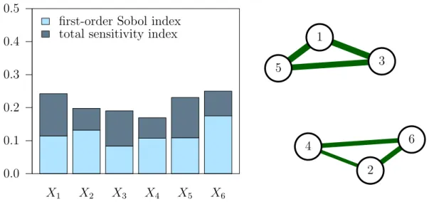
With the TII, it is possible to discover the block-additive structure of the underlying function, that is we can identify a decomposition into groups of input variables such that variables between groups do not interact. As an illustration, we analyze the following function,
f(X1, . . . , X6) = cos([1, X1, X3, X5]α) + sin([1, X2, X4, X6]γ),
with Xi i.i.d.
∼ U[−1,1], i = 1, . . . ,6, α = [−0.8,−1.1,1,1.1]0 and γ = [−0.51,0.9,−1.1]0, where the prime 0 stands for the transpose.
Clearly, the variables in the group {X1, X3, X5} do not interact with the variables in the group {X2, X4, X6}, which induces a block-additive structure of the form f(x) = f135(x1, x3, x5) + f2,4,6(x2, x4, x6). This, however, cannot be seen from the common first-order and total sensitivity indices (Fig. 3.1, left). We only see that all variables have first-order and total effects, but do not know how variables interact with each other.
If we now estimate the TII for each combination of input variables, we obtain such information, which can be conveniently plotted in a so-called FANOVA graph in Fig. 3.1 on the right (M¨uhlenst¨adt et al., 2012). The TII of the two variables is represented by
27 X1 X2 X3 X4 X5 X6 0.0 0.1 0.2 0.3 0.4 0.5
first-order Sobol index
total sensitivity index 1
2 3
4 5
6
Figure 3.1: Sensitivity analysis of the motivational example. First-order Sobol and total sensitivity indices (left), FANOVA graph of total interaction indices (right).
the thickness of the edge between the two corresponding vertices. With the graph, the partition into the two additive groups is clearly visible.
This information about the block-additive interaction structure of a function can be exploited in several fields of computer experiment analysis. M¨uhlenst¨adt et al. (2012) show that it can be used to improve Kriging model predictions by adapting the Kriging kernel to the block-additive structure. For the example above that would mean to modify the kernel k from Equation (2.3) as follows,
k(h) = k1(h2, h4, h6) +k2(h1, h3, h5).
Furthermore, the block-additive structure can be exploited to simplify and parallelize optimization, as described in Ivanov and Kuhnt (2014). There, the idea is to optimize the separate groups independently, which reduces the optimization dimensions and enables parallelization, an important property as optimization techniques are usually sequential. For the example above, the six-dimensional optimization problem of mini-mizingf simplifies into two three-dimensional ones, where the c1, . . . , c6 are constants,
which are not varied in the optimization, min x1,...,x6 f(x1, . . . x6) = min x1,x3,x5 f(x1, c2, x3, c4, x5, c6) + min x2,x4,x6 f(c1, x2, c3, x4, c5, x6).
3.1
Total interaction indices
The TII measures the total influence of a second-order interaction between two input variables. It contains, for any pair of input variables, the influence of their interaction plus all interactions containing both indices. This is different from the second-order Sobol index (2.8), which does not contain higher interactions, and from the second-order total sensitivity index (2.10), which additionally contains first-second-order effects as well as higher-order interactions of only one of the two variables.
Definition 3.1. The total interaction index (TII) of two input variables Xi and Xj is
defined by Di,j =Var X I⊇{i,j} fI(XI) = X I⊇{i,j} DI. (3.1)
The TII is a special second-order version of the more general superset importance, which was introduced by Liu and Owen (2006) for uniform distributions (Υ2u) as a measure of importance of interactions and their supersets. It was also investigated by Hooker (2004) in the data mining framework (σ2u). The superset importance Υ2u is defined for any subset u⊆ {1, . . . , d} as
Υ2u =σ2u =X I⊇u
DI. (3.2)
One important property of the TII is its link to total sensitivity indices and closed indices respectively.
3.1 Total interaction indices 29 Proposition 3.1. Di,j = DTi +D T j −D T i,j, (3.3)
Di,j = D+DC−{i,j}−D−iC −DC−j. (3.4)
Proof. The proof of (3.3) is obtained by simple set transformation. Since
X I⊇{i}∨I⊇{j} DI = X I⊇{i} DI + X I⊇{j} DI− X I⊇{i,j} DI, it holds that X I⊇{i,j} DI = X I⊇{i} DI+ X I⊇{j} DI− X I⊇{i}∨I⊇{j} DI.
Equation (3.4) then can be deduced from (3.3) using the connection between total and closed indices (2.13), Di,j = DTi +D T j −D T i,j = (D−DC−i) + (D−D−jC )−(D−D−{i,j}C ) = D+DC−{i,j}−D−iC −DC−j.
From the connection to the superset importance, another representation of the TII is given by Liu and Owen (2006).
Proposition 3.2. Liu and Owen’s formula Di,j = 1 4E f(Xi, Xj,X−{i,j})−f(Xi, Zj,X−{i,j}) −f(Zi, Xj,X−{i,j}) +f(Zi, Zj,X−{i,j}) 2i , (3.5)
Proof. A proof is given in Liu and Owen (2006). In addition, (3.5) can be connected to (3.4). When expanding the squared sum in (3.5), of the 10 resulting terms the four squared terms are simply equal to E(f(X)2) =D+f2
0. The six double products gather two by two, and result in the pick-freeze formula (2.15)
• E[f(Zi, Xj,X−{i,j})f(Zi, Zj,X−{i,j})]
=E[f(Xi, Xj,X−{i,j})f(Xi, Zj,X−{i,j})] =DC−j+f02 • E[f(Xi, Zj,X−{i,j})f(Zi, Zj,X−{i,j})]
=E[f(Xi, Xj,X−{i,j})f(Zi, Xj,X−{i,j})] =DC−i+f02 • E[f(Zi, Xj,X−{i,j})f(Xi, Zj,X−{i,j})]
=E[f(Xi, Xj,X−{i,j})f(Zi, Zj,X−{i,j})] =D−{i,j}C +f02 Finally, combining all the terms gives (3.4).
Remark: Connection to ANOVA Liu and Owen (2006) state that formula (3.5)
“can also be obtained through the classical formulas for expected mean squares in the discrete ANOVA as established by Cornfield and Tukey (1956)”. This connection becomes evident when looking at the formula for the interaction Sum of Squares in an ANOVA with two input variables A and B (Cornfield and Tukey, 1956, p. 916),
SSAB =n a X i=1 b X j=1
(¯yij·−y¯i··−y·j·¯ + ¯y···)2,
with aand b the number of levels and yijk, i= 1, . . . , a, j = 1, . . . , b, k = 1, . . . , nthe realized output values with n the number of repetitions.
For a further TII computation notion, say we keep all variables other thanXi and Xj fixed and look at the Liu and Owen formula for the resulting two-dimensional function ffixed(Xi, Xj),
Di,j = 1 4E
(ffixed(Xi, Xj)−ffixed(Xi, Zj)−ffixed(Zi, Xj) +ff ixed(Zi, Zj))2
3.2 TII estimation 31
Then we see that the TII of the original function can be computed as the expected value over this second-order interaction index of the two-dimensional function obtained by fixing all variables exceptXiandXj. Thus, the Liu and Owen formula is a so-called
fixing method, introduced by M¨uhlenst¨adt et al. (2012).
Proposition 3.3. (Fixing method). For anyx−{i,j}, defineffixedas the two-dimensional function ffixed : (xi, xj)→ f(x) obtained from f by fixing all input variables except xi
and xj. Let Di,j|X
−{i,j} denote the second-order Sobol index of ffixed(Xi, Xj), which
depends on the fixed variables X−{i,j}. Then the TII of Xi and Xj is obtained by
integrating Di,j|X
−{i,j} with respect to X−{i,j},
Di,j =E Di,j|X −{i,j} . (3.6)
Proof. Since the function ffixed is two-dimensional, it has only one interaction, which is a second-order one, and coincides with its TII. Hence, this interaction can be computed by applying (3.5) to ffixed,
Di,j|X
−{i,j} = 1
4E [ffixed(Xi, Xj)−ffixed(Xi, Zj)−ffixed(Zi, Xj) +ffixed(Zi, Zj)] 2
.
Now we can rewrite the right hand side by using conditional expectations, Di,j|X
−{i,j} = 1 4E
f(Xi, Xj,X−{i,j})−f(Xi, Zj,X−{i,j})
−f(Zi, Xj,X−{i,j}) +f(Zi, Zj,X−{i,j})2|X−{i,j}
i
.
Taking the expectation with respect to X−{i,j} gives the result.
3.2
TII estimation
The different representations of the TII derived in the last section and the estima-tion methods of the common indices from Secestima-tion 2.3 are now combined to construct estimation methods for the TII, followed by remarks on their properties.
Estimation via total sensitivity indices
To apply the link between the TII and total sensitivity indices from Prop. 3.1, formula (3.3), estimators for the total sensitivity index of first- and second-order are required. Thus, either the Monte Carlo estimator via the Jansen formula (2.23) or the RBD-FAST method (2.29) can be used, resulting in the TII estimatorsJansen TII estimator
and RBD-FAST TII estimator,
Jan b Di,j = Jan b DTi +JanDbjT − Jan b DT{i,j} (3.7) RBD b Di,j = RBD b DiT +RBDDbjT − RBD b D{i,j}T (3.8)
For the Jansen TII estimator, evaluations can be saved by computing the last term Jan
b
DT
{i,j} via f(x−i,zi) and f(x−j,zj), which have been evaluated in the computation of the previous terms, rather than via f(x) and f(x−{i,j},z{i,j}). The approach is discussed further in Section 3.4.
Estimation via closed sensitivity indices
The second link from Prop. 3.1 between the TII and the closed sensitivity indices (3.4) requires the estimation of high-order closed indices DC−i and Di,jC. To this point, no reliable FAST or RBD-FAST method exists, so Monte Carlo integration is considered. As the required closed indices are of high order, they are expected to be large. Thus, the estimator based on the pick-freeze formula (2.15, 2.16) is more suitable here than the one based on the strategies fromCorrelation 1 andCorrelation 2 (2.21) since they are not recommended when the index to be estimated is rather large (Owen, 2013a). The pick-freeze TII estimator of the TII is constructed as
pf b Di,j =Db + pf b DC−{i,j}−pfDbC−i− pf b DC−j. (3.9)
3.2 TII estimation 33
As for the Jansen TII estimator, evaluations can be reused in the second-order term by using f(x−i, zi) and f(x−j, zj) rather than f(x) and f(x−{i,j},z{i,j}).
Estimation via Liu and Owen’s formula
Another TII estimation method is directly obtained by Liu and Owen’s formula in Prop. 3.2, the Liu and Owen TII estimator
LO b Di,j = 1 4× 1 n n X k=1 f(xki, xkj,xk−{i,j})−f(xki, zjk,xk−{i,j}) −f(zik, xkj,xk−{i,j}) +f(zki, zjk,xk−{i,j})2. (3.10)
Estimation via fixing method
Following Prop. 3.3, the TII can be computed by averaging the second-order interaction of two-dimensional functions in the way it has been done in M¨uhlenst¨adt et al. (2012) by the following scheme:
Let us consider a couple of integers (i, j), with i < j. Fork = 1, . . . , nMC carry out the following steps.
1. Simulate xk−{i,j} from the distribution of X−{i,j}, that is take a single sample of all input variables except Xi and Xj.
2. Create the two-dimensional function ff ixed by fixing f on xk−{i,j} ffixed(Xi, Xj) =f(xk1, . . . , Xi, . . . , Xj, . . . , xkd).
3. Using the FAST estimator (Section 2.3.3), compute the second-order Sobol index of ffixed, denoted Dbk i,j|X−{i,j} , by b Dki,j|X −{i,j} = FAST b D|kX −{i,j}− FAST b Di|kX −{i,j}− FAST b Dj|kX −{i,j},
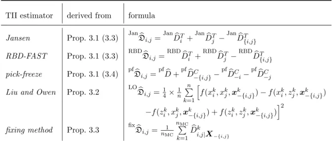
TII estimator derived from formula
Jansen Prop. 3.1 (3.3) JanDbi,j =
Jan b DiT +JanDbTj − Jan b D{i,j}T RBD-FAST Prop. 3.1 (3.3) RBDDbi,j =
RBD b DiT +RBDDbTj − RBD b DT{i,j} pick-freeze Prop. 3.1 (3.4) pfDbi,j =
pf b D+pfDbC−{i,j}− pf b DC −i− pf b DC −j Liu and Owen Prop. 3.2 LODbi,j = 1
4× 1 n n P k=1 h f(xki, xkj,xk−{i,j})−f(xki, zkj,xk−{i,j}) −f(zik, xkj,xk−{i,j}) +f(zik, zkj,xk−{i,j})i2
fixing method Prop. 3.3 fixDbi,j = n1 MC nMC P k=1 b Di,j|k X −{i,j}
Table 3.1: Overview of considered TII estimators.
whereDbk
|X−{i,j}
denotes the overall variance offfixedandDbk
i|X−{i,j}
andDbk
j|X−{i,j} the first-order indices of Xi and Xj, respectively.
After carrying out the three points for all k = 1, . . . , nMC, compute the fixing method
TII estimator by fix b Di,j = 1 nMC nMC X k=1 b Dki,j|X −{i,j}. (3.11)
A summary of all considered TII estimators can be found in Tab. 3.1.
3.3
Theoretical properties of TII estimators
In the following, the introduced TII estimators are compared according to different statistical properties.
3.3 Theoretical properties of TII estimators 35
Nonnegativity
As the indices measure the sum of variances, the estimates should be nonnegative. This holds for the Liu and Owen TII estimator (3.10) which is a sum of squares. However, negative estimates can occur for the Jansen (3.7), the pick-freeze (3.9) and the RBD-FAST TII estimator (3.8). For thefixing method TII estimator (3.11), there is a sufficient condition, which results from the following proposition:
Proposition 3.4. Let f be a two-dimensional function, and consider its second-order interaction D12 =D−D1−D2. Denote by Db12 = FAST b D−FASTDb1− FAST b D2 its FAST
estimate (see Section 2.3.3) and assume that:
(i) ω1 and ω2 are free of interference up to order 2M,
(ii) N ≥2M ×max(ω1, ω2). Then Db12≥0.
Proof. Denote the sets Wωi,M = {pωi, p = 1, . . . , M} for i = 1,2, and WN =
{1, . . . , N/2}. With (2.27) and (2.28), we have
b D12/2 = X n∈WN (Ab2n+Bbn2)− X n∈Wω1,M (Ab2n+Bbn2)− X n∈Wω2,M (Ab2n+Bbn2).
Now, the condition (i) ensures thatWω1,M∩Wω2,M =∅while (ii) implies thatWωi,M ⊆
WN, fori= 1,2. Hence, b D12/2 = X n∈WN −(Wω1,M∪Wω2,M) (Ab2n+Bbn2)≥0.
It is a direct consequence of Prop. 3.4 that if (i) and (ii) are satisfied, then (3.11) returns positive values. In practice, one can use for instance ω1 = 11, ω2 = 35 (Mara, 2009), which are free of interferences up to 2M for the usual orders M = 4,6. Then the minimal value of N is 2×6×max{11,35}= 420.
Bias
The methods based on direct Monte Carlo estimation, Jansen and Liu and Owen TII estimator, are unbiased since only direct mean estimators are used for the conditional expectations. This is especially remarkable in combination with the positivity of theLiu and Owen TII estimator, as it implies that when the true value is zero, the estimator is identical to zero as well.
Proposition 3.5. If Di,j = 0, then the Liu and Owen TII estimator is equal to zero:
LO
b
Di,j ≡0.
Proof. Starting with the FANOVA decomposition (2.4), if Di,j = 0, then all of the terms containing bothxi and xj vanish. So the decomposition reduces to
f(x) = X i /∈I∧j /∈I fI(xI) + X i∈I∧j /∈I fI(xI) + X i /∈I∧j∈I fI(xI) = a0(x−{i,j}) +ai(xi,x−{i,j}) +aj(xj,x−{i,j}).
Inserting this representation of f into the squared term of the Liu and Owen TII estimator (3.10) returns zero,
f(xki, xkj,xk−{i,j})−f(xki, zjk,xk−{i,j})−f(zki, xkj,xk−{i,j}) +f(zik, zjk,xk−{i,j}) =ai(xki,xk−{i,j})−ai(xki,xk−{i,j})−ai(zik,xk−{i,j}) +ai(zik,xk−{i,j})
+aj(xkj,xk−{i,j})−aj(zjk,xk−{i,j})−aj(xkj,xk−{i,j}) +aj(zjk,xk−{i,j}) = 0.
In the pick-freeze TII estimator, the estimation of f2
0 is necessary in the estimation of the closed sensitivity indices (2.16). If we estimatef02 by taking the square of fb0 (2.17)
or*fb0 (2.19), we introduce a bias of −Var(f0), as was noted by Owen (2013b),
[E(f0)] 2
= E(f0) 2
3.3 Theoretical properties of TII estimators 37
However, as long as E(f(X)4)<∞, the bias is asymptotically negligible. Owen (2013b) remarks that the bias may be important in the case of small closed sensitivity indices, but those are not expected in the estimation ofpfDbi,j, as mentioned in Section 3.2. To
nonetheless ensure unbiasedness, unbiased estimators for the closed sensitivity index can be used such as Cor1DbCI or
Cor2
b
DC
I or (2.21), which do not need an estimate of f02, or the estimator eτ2 proposed in Section 7 of Owen (2013b).
Frequency-based estimators are generally prone to bias (Tissot and Prieur, 2012). This bias might even be enhanced here through the use of a combination ofFAST estimators for thefixing method TII estimator andRBD-FAST estimators for theRBD-FAST TII estimator.
Asymptotic properties of the Liu and Owen TII estimator
Corresponding to the asymptotic properties of the pick-freeze estimator of closed sen-sitivity indices (end of Section 2.3.2), it is possible to derive asymptotic properties of the Liu and Owen TII estimator (3.10). To do this, the estimator for a pair of input variables {Xi, Xj}is written as
Tn= LO b Di,j = 1 n n X k=1 ∆k i,j 2 4 , with
∆ki,j =f(Xik, Xjk,Xk−{i,j})−f(Xik, Zjk,Xk−{i,j})−f(Zik, Xjk,Xk−{i,j})
+f(Zik, Zjk,Xk−{i,j}).
Proposition 3.6. LetP be the set of all cumulative distribution functions of exchange-able random vectors in L2(R2), that is for a P ∈ P it holds for any random vectors X
and X0 that P(X, X0) = P(X0, X). Then the following propositions hold for the Liu and Owen TII estimator Tn.
a) Tn is consistent for Di,j,
Tn a.s. −→ n→∞ Di,j.
b) Tn is asymptotically normally distributed,
√ n(Tn−Di,j) d −→ n→∞ N 0,Var[(∆ 1 i,j)2] 16 .
c) Tn is asymptotically efficient in the notion of van der Vaart (1998) for estimating
Di,j for P ∈ P.
Proof. The results a) and b) are a direct application of the law of large numbers and the central limit theorem, applied to the variables (∆ki,j)2.
Result c) follows from the fact that estimators with symmetrical expressions are asymp-totically efficient in the framework of exchangeable variables, as proved by Janon et al. (2013) in their Lemma 2.6 (2):
Let Φ2 :R2 →R be a symmetric function in L2(P) and f a deterministic function on
R ⊂Rp1+p2 of independent random input variables X ∈
Rp1 and Z ∈Rp2. Z0 denotes
an independent copy of Z and Xk,Zk,Z0k, k = 1, . . . , n denote independent samples of the corresponding variables. The sequence {Φ2
n}n∈N given by Φ2n= 1 n n X k=1 Φ2 f(Xk, Zk), f(Xk, Zk0)
is asymptotically efficient for estimating E(Φ2(f(X, Z), f(X, Z 0
))) for P ∈ P. More precisely, denote Xk = (Xjk, Zjk,X
k
−{i,j}), Zk = Xik, Z 0
k =Zik, and let g be the function defined over Rd×
R by g(a, b) =f(b, a1, a3, . . . , ad)−f(b, a2, a3, . . . , ad). Then ∆ki,j =g(Xk,Zk)−g(Xk,Z 0 k).
3.3 Theoretical properties of TII estimators 39 Therefore Tn= 1 n n X k=1 Φ2(g(Xk,Zk), g(Xk,Zk0)), and Di,j = E(Φ2(g(X1,Z1), g(X1,Z 0 1))),
where Φ2 is the two-dimensional function defined overR2 Φ2(u, v) =
(u−v)2
4 .
Remark thatZk andZ 0
k are independent copies of each other, both independent ofXk, and that Φ2 is a symmetric function. With the following change in notation
i←k, X ←X, Z ←Z, Z0 ←Z0, f ←g
the result follows from the Lemma of Janon et al. (2013) named above.
The two last propositions can be extended to the general superset importance (3.2), including the case of the total sensitivity index of one input variable.
Proposition 3.7. Let ΥI =PJ⊇IDJ be the superset importance for a set I. Define TI,n = 1 n n X k=1 (∆k I)2 2|I| , with ∆kI =P J⊆I(−1)|I−J|f(Z k J,X k
−J), where |.| stands for the number of elements in
a set and A−B ={x|x∈A and x /∈B} denotes the difference of two sets A and B. Then TI,n is asymptotically normal and asymptotically efficient for ΥI.
Proof. Note that TI,n is the sample version of the formula (10) given by Liu and Owen (2006) for ΥI (with suitable change of notations). The proof of asymptotic normality is thus a direct consequence of the central limit theorem. For asymptotic efficiency, the proof relies on arguments similar to Prop. 3.6.
• When I ={i}is a single input variable, we have
∆kI =f(Zik,X−ik )−f(Xik,Xk−i), which is of the formg(Xk,Zk)−g(Xk,Z
0
k) with Zk =Zik, Z 0
k=Xik,Xk =Xk−i, and g(a, b) = f(b,a).
• When |I| ≥ 2, let us choose i ∈ I. Then, by splitting the subsets of I into two parts, depending whether they contain {i}, we have
∆kI = X J⊆I−{i}
(−1)|I−J|f(ZkJ,Xk−J)
+ X
J⊆I−{i}
(−1)|I−(J∪{i})|f(ZkJ∪{i},Xk−(J∪{i}))
= X J⊆I−{i} (−1)|I−J|f(ZkJ, Xik,Xk−(J∪{i})) − X J⊆I−{i} (−1)|I−J|f(ZkJ, Zik,Xk−(J∪{i})),
which is also of the formg(Xk,Zk)−g(Xk,Z 0
k) withZk =Xik, Z 0
k =Zik,Xk = (XkI−{i},ZkI−{i},Xk−I), and a suitable g since the second term in the difference is obtained from the first one by exchangingXk
i and Zik.
The result is then obtained by applying Lemma 2.6 in Janon et al. (2013) to the symmetric function Φ2(u, v) =
(u−v)2
2|I| , remarking that Zk and Z 0
k are independent copies of each other, both independent of Xk.
Corollary 3.1. It follows from Prop. 3.7 that the Jansen estimator of the total sensi-tivity index of a single variable DT
3.4 Estimating the full set of TIIs 41
3.4
Estimating the full set of TIIs
In most of the practical applications, the full set of d(d−1)2 TIIs, that is the TII of each possible pair of the d input variables, is required simultaneously. The function evaluations, especially in the case without a metamodel, where f represents the actual computer experiment, are usually the most time-consuming part of the estimation. Table 3.2 therefore gives an overview of the number of evaluationsN that are required by each method for the estimation of the full set of TIIs, depending on the different parameter settings for each method.
In each of the n Monte Carlo runs, the Liu and Owen TII estimator requires one es-timate corresponding to f(x), d estimates corresponding to f(zi,x−i) — and at the same time to f(zj,x−j) — and d2
estimates corresponding to f(zi, zj,x−{i,j}). Simi-larly, theRBD-FAST TII estimator requiresdestimates ofRBDDbTi and d2
estimates of RBD
b
DT
{i,j}, and each estimate requires a number of 2(M d+L) runs. The fixing method
TII estimator requires for each of the d2 indices a number of nM C FAST estimates. For the Jansen and the pick-freeze TII estimator, strategies that reuse computations corresponding to the strategy by Saltelli (2002) (Section 2.3.2) can be applied, as addressed in their definitions (3.7) and (3.9). In the estimation of the first- and second-order total indices for the Jansen TII estimator as well as in the estimation of the (d− 1)- and (d −2)-order closed indices for the pick-freeze TII estimator, only the (d+ 1)n samples f(xk) and the f(zk
i,xk−i), 1≤k ≤n, 1≤i ≤d are required for the estimation of all TII indices. In addition, those function evaluations can be used to estimate the full set of first-order total sensitivity indices using either (2.22) or (2.23). By adding only the n samplesf(zk), 1≤k ≤n, all first-order Sobol indices (2.16) can be estimated as well.
Table 3.2 clearly shows that in contrast to the other estimators, the Jansen as well as the pick-freeze TII estimator are scalable in the sense that the number of required runs increases linearly with the number of input variables d.