A modified indicator-based evolutionary algorithm (mIBEA)

(1)

Li, Wenwen and Özcan, Ender and John, Robert and

Drake, John H. and Neumann, Aneta and Wagner,

Markus (2017) A modified indicator-based evolutionary

algorithm (mIBEA). In: IEEE Congress on Evolutionary

Computation 2017, 5-9 June 2017, Donostia-San

Sebastian, Spain.

Access from the University of Nottingham repository:

http://eprints.nottingham.ac.uk/41420/1/A%20Modified%20Indicator-based%20Evolutionary

%20Algorithm%20%28mIBEA%29%20final%20submission.pdf

Copyright and reuse:

The Nottingham ePrints service makes this work by researchers of the University of

Nottingham available open access under the following conditions.

This article is made available under the University of Nottingham End User licence and may

be reused according to the conditions of the licence. For more details see:

http://eprints.nottingham.ac.uk/end_user_agreement.pdf

A note on versions:

The version presented here may differ from the published version or from the version of

record. If you wish to cite this item you are advised to consult the publisher’s version. Please

see the repository url above for details on accessing the published version and note that

access may require a subscription.

(2)

A Modified Indicator-based Evolutionary Algorithm

(

m

IBEA)

Wenwen Li, Ender ¨

Ozcan, Robert John

School of Computer Science University of Nottingham Jubilee Campus, Wollaton Road,

Nottingham, UK, NG8 1BB Email: [email protected]

[email protected] [email protected]

John H. Drake

Operational Research Group Queen Mary University of London

Mile End Road, London, UK, E1 4NS Email: [email protected]

Aneta Neumann, Markus Wagner

School of Computer Science The University of Adelaide

Ingkarni Wardli Building, Adelaide, Australia SA 5005 Email: [email protected]

[email protected]

Abstract—Multi-objective evolutionary algorithms (MOEAs) based on the concept of Pareto-dominance have been successfully applied to many real-world optimisation problems. Recently, research interest has shifted towards indicator-based methods to guide the search process towards a good set of trade-off solutions. One commonly used approach of this nature is the indicator-based evolutionary algorithm (IBEA). In this study, we highlight the solution distribution issues within IBEA and propose a modification of the original approach by embedding an additional Pareto-dominance based component for selection. The improved performance of the proposed modified IBEA (mIBEA) is empirically demonstrated on the well-known DTLZ set of benchmark functions. Our results show that mIBEA achieves comparable or better hypervolume indicator values and epsilon approximation values in the vast majority of our cases (13 out of 14 under the same default settings) on DTLZ1-7. The modification also results in an over 8-fold speed-up for larger populations.

I. INTRODUCTION

In multi-objective optimisation, where multiple objectives are optimised simultaneously, the goal is to find a set of

P areto-optimal solutions known as the Pareto front (PF). The PF consists of a set of solutions that are not dominated by each other, which are termed asnon-dominatedsolutions, represent-ing the trade-off that exists between different objectives. This dominance relation, also known asPareto dominancerelation, (≺) is defined between solutions x1 _and_x2_{. We say w.l.o.g.,} in a minimisation problem that x1 _dominates _x2 ₍_x1 _≺ _x2₎ if and only if fi(x1) ≤ fi(x2) for all k objective functions

(i∈ {1, . . . k}), andfi(x1)< fi(x2)for at least one objective

function. One of the difficulties in multi-objective search is to find a set of solutions to minimise the distance to the true Pareto front (PF) while maintaining the diversity of the solution set in the objective space.

Multi-objective evolutionary algorithms (MOEAs) are widely used to solve various multi-objective optimisation problems [16] and are considered to be general and robust search mechanisms [1]. Evolutionary algorithms (EAs) are a class of stochastic optimisation methods that mimic the process of evolution in nature. Examples of EAs, such as genetic algorithms, evolutionary programming, and evolution

strategies [1] operate on a set of solutions using the ba-sic principles of natural evolution: selection, reproduction by means of recombination and mutation. The algorithmic difference between single-objective EAs and MOEAs is that additionally in an MOEA, the multiple objectives of a solution must be transformed into a single fitness value to facilitate the comparison of individual solutions [6]. Thus, MOEAs often vary in the method of this transformation, considering the balance of convergence and diversification during the search. Some MOEAs, such as NSGA-II [7], SPEA2 [18], and AGE [3, 13] incorporate Pareto-based ranking of the individuals and an additional density measurement (crowding

distance in NSGA-II, k-th nearest neighbour in SPEA2,

-dominancein AGE) in the objective space. However, between

two non-dominated solutions, purely Pareto-based MOEAs are not able to ascertain which solutions have better potential for convergence. IBEA [17] was one of the earliest indicator-based MOEAs proposed in the literature. Originally, it came in two variants: one using-dominance for guidance, denoted IBEA,

and another based on hypervolume, denoted IBEAHD (‘HD’

stands for hypervolume difference) which will be referred to as IBEA from this point onward in this study. IBEA associates a fitness value with each solution based on the selected indicator (hypervolume or ), attempting to guide the search towards the true PF. IBEA was shown to achieve significantly better performance on various benchmark functions than NSGA-II and SPEA2 [17], however the distribution of the solutions found by IBEA has rarely been reported or discussed in detail. In this paper, we propose a modified variant of IBEAHD,

termed mIBEA, which adds a Pareto-based element to this indicator-based method, analysing the distribution of non-dominated solutions found. For further information about MOEAs and indicator-based MOEAs in particular, we refer the interested reader to [5, 6, 16].

The remainder of the paper is structured as follows. We first describe the original IBEA in Section II-A, then present ob-servations of the solution distributions observed using existing MOEAs in Section II-B. The proposedmIBEA is introduced in Section III. Experimental results comparing IBEA andmIBEA are presented in Section IV. We draw conclusions and provide

(3)

ideas for future work in Section V.

II. INDICATOR-BASEDEVOLUTIONARYALGORITHM

Since the focus in the paper is on the hypervolume variant of IBEA, i.e. IBEAHD, we first give a detailed description of

the original IBEA. We then provide visualisations and obser-vations for the non-dominated solution sets found using IBEA and two other existing MOEAs, one Pareto dominance-based (NSGA-II [7]) and one indicator-based (SMS-EMOA [2]).

A. Description of IBEA

The core idea of IBEAHD is to employ a binary

hyper-volume indicator in the selection process, when determining which solutions survive to the next generation. The binary hypervolume indicator assigns a real-valued number to two solution sets with respect to a reference point. The formula of

IHD(A, B)is defined as space that is dominated by population B, but not byA, shown in Equation (1) [17].

IHD(A, B) =

(

IH(B)−IH(A),∀x2∈B∃x1∈A:x1≺x2 IH(A+B)−IH(A), o.w.

(1) where IH(A) denotes the hypervolume formed by the

solution set A. Correspondingly, IH(A+B) means the

hy-pervolume of the union of solution set A andB.IHD(A, B)

is negative if all solutions inB are dominated by solutions in

A. Note thatIH(A)6=IH(B).

The pseudocode of the original IBEA is given in Alg. 1. IBEA first randomly generates an initial population in Step1, then the following steps loop until the stopping criterion is satisfied. The objective values are scaled and the fitness is assigned to each individual in Step2 and Step3. Step4 performs environmental selection, iteratively removing the worst individual in the populationP based on indicator value untilµindividuals remain (this step will do nothing in the first iteration of the algorithm as P =µ). Upon removal of each solution, the indicator values of the remaining solutions must be updated. This step continues until the number of solutions inP does not exceedµ. The standard mating selection (Step6) and variation (Step7) steps are performed to generate new individuals and add them to the population P.

B. Solution distribution issues in existing MOEAs

It is common in the MOEA literature to use various quantitative indicators, such as hypervolume,-approximation and inverted generational distance (IGD) [19], to compare the performance of different MOEAs. However, the distribution of non-dominated solutions over the resultant solution fronts is relatively rarely reported, at least in part due to the lack of quantitative indicators to measure it in the objective space.

One method for measuring the spread of solutions over the objective space we will use here is Generalised Spread (GS) [15]. GS computes the average Euclidean distance of any two consecutive solutions [7] (or nearest neighbours in [15]) in the population, and considers this average in the context of the minimal achieved distances to the extreme points of the true

Algorithm 1:(Adaptive) IBEAHD as described in [4, 17]

Inputs:

µ: population size;

N: number of total solution evaluations;

ρ: objective values scaling factor;

κ: indicator value (hypervolume difference) scaling factor Output:A: Pareto set approximation

Step1: Initialisation: Randomly generate the initial population P and set up evaluation counter m. Step2: Scale objective values:

1) find the lower (bi=minx∈Pfi(x)) and upper

(bi=maxx∈Pfi(x)) bound of each objective i.

2) increase the upper boundbi

0

=bi+ρ∗(bi−bi)

3) scale each objective to the interval [0, 1];

f_i0 = (fi(x)−bi)/(bi

0

−bi)

Step3: Fitness Assignment:

1) calculate indicator valuesI(x1_{, x}2₎_{using the scaled} objective values f_i0 instead of original objective values

fi, and determine the maximum absolute indicator value c=maxx1,x2_∈P|I(x1, x2)|

2) compute the fitness for allx1∈P,

F(x1) =P

x2_∈_P_\_x1−exp−I(x

2_,x1₎_/c_∗_κ

Step4: Environmental Selection: iterate the following three sub-steps until the size of population P ≤µ. 1) choose an individualx?_∈_P _{with the smallest fitness}

value, i.e., F(x?₎_≤_F₍_x₎_{for all}_x_∈_P

2) removex? _from_P

3) update fitness values of all the remaining individuals

x∈P as F(x) =F(x) + exp−I(x?,x)/c∗κ

Step5: Termination criteria: ifm≥N, return the

non-dominated solutions inP asA; otherwise, continue. Step6: Mating Selection: apply binary tournament

selection operator to P to select two parents fromP. Step7: Variation: perform crossover operator on the two

parents to generate two offspring, and use an mutation operator on one of the offspring. The resulting offspring is then added toP. Increment iteration counter

(m=m+ 1). Go to Step 2.

PF. The smaller the value of GS, the better spread the resultant front has as the variance is reduced and/or points closer to the extreme points have been found. The ideal spread is achieved when GS equals to 0 as this means that the extreme points are found and the solutions are evenly spread out.

In this study, for the purpose of analysis, we also use a new metric –border fraction (bf) to provide a certain quantitative measurement of the solution distribution of different PFs. We defineborder fractionas the fraction of non-dominated points lying in a pre-defined border or area of the resultant PF. More precisely, assume the lower bound of each objective function is 0, the border threshold for each objective is denoted asθi, then

the border is the volume defined by(0< f1≤θ1||0< f2≤

θ2||, ...,||0< fk≤θk), wherekis number of objectives in the

(4)

the population, the border fractionbfvalue is the proportion of non-dominated individuals in the population which lie within in this border. Note thatbf is not a general metric to measure the solution distribution of a Pareto optimal (or approx.) set.

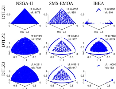
As a motivating example, we apply three well-known MOEAs, NSGA-II, SMS-EMOA and IBEA, to a sample of three DTLZ problems [8], using the default settings for each method. Figure 1 shows the non-dominated solutions found in 100 independent runs for each MOEA on each problem, except for SMS-EMOA which was run only 10 times due to its high running time. The maximum number of evaluations for each run was 100,000. The bf and ndi values are also provided on the top right corner of each plot.

NSGA-II SMS-EMOA IBEA

DTLZ1 0 0 0 0.5 0.5 0.5 bf: 0.4745 ndi: 9179 0 0 0 0.5 0.5 0.5 bf: 0.4352 ndi: 988 0 0 0 0.5 0.5 0.5 bf: 0.9935 ndi: 616 DTLZ2 0 0 0 0.5 0.5 0.5 1 1 1 bf: 0.2229 ndi: 5550 0 0 0 0.5 0.5 0.5 1 1 1 bf: 0.5451 ndi: 987 0 0 0 0.5 0.5 0.5 1 1 1 bf: 0.7186 ndi: 8924 DTLZ3 0 0 0 0.5 0.5 0.5 1 1 1 bf: 0.2211 ndi: 7134 0 0 0 0.5 0.5 0.5 1 1 1 bf: 0.5216 ndi: 947 0 0 0 0.5 0.5 0.5 1 1 1 bf: 1.0000 ndi: 182

Fig. 1: Comparison of non-dominated solution sets for NSGA-II, SMS-EMOA and IBEA.

Firstly, we can see that the solutions from NSGA-II can cover the whole fronts of all the problems DTLZ1-3. Secondly, SMS-EMOA can reach almost full coverage of the PF for DTLZ1, however, on DTLZ2 and 3 the PFs have clear gaps between the border and central area. Thirdly, similar to SMS-EMOA, IBEA also shows clear gaps (empty space) on the PF of DTLZ2. Also, solutions by the original IBEA are heavily concentrated in the corner points on DTLZ1 and DTLZ3.

The GS measurement of the solution fronts obtained from NSGA-II, SMS-EMOA and IBEA (as illustrated in Figure 1) is shown in Table I. The best GS on each benchmark func-tion is highlighted in bold. Not surprisingly, IBEA performs poorly w.r.t. GS among all the three algorithms on DTLZ1-3. However, interestingly, although SMS-MOEA shows gaps on the resultant PFs of DTLZ2 and 3, the GS indicator still shows that it performs best on both problems. This suggests that under certain situations (e.g., PFs of DTLZ2 and 3 from SMS-EMOA) GS cannot capture the distribution of the PF, i.e., the spread calculated is not equivalent to the distribution. In the following, we usebfandndito capture the bias within the distribution towards extreme points on the solution fronts. The border threshold is set as 0.03 for DTLZ1 and 0.1 for both

TABLE I: Generalised SpreadM eanstd values for NSGA-II,

SMS-EMOA and IBEA on DTLZ1-3.

Generalised Spread NSGA-II SMS-EMOA IBEA DTLZ1 0.57740.30 0.07800.01 1.38350.38 DTLZ2 0.49510.04 0.23930.02 0.47050.03 DTLZ3 0.52840.09 0.23880.02 1.59210.30

DTLZ2 and 3. These parameters are determined by the gaps or corner points from IBEA illustrated in Figure 1. We can see that for IBEA, on DTLZ1 and DTLZ3 almost all points lie in the border area of IBEA, and 72% of points are in the border area for DTLZ2. SMS-EMOA shows good PF coverage on DTLZ1, but a biased solution distribution is obvious on the outside ‘ring’ area and the inside central area in DTLZ2 and DTLZ3. Interestingly, the Pareto dominance-based MOEA NSGA-II shows good PF coverage and fairly uniform solution distributions on DTLZ1-3. In addition, IBEA only identifies 616 non-dominated solutions when solving DTLZ1 and 182 for DTLZ3 after 100 independent runs, which is significantly less than thendivalues of NSGA-II on these instances (9179 for DTLZ1 and 7134 for DTLZ3).

To the best of our knowledge, even though these uneven solution distributions have been plotted in articles before, e.g. [2, 12], no further details are discussed in those papers. Although IBEA is often reported as having exceptional in-dicator value performance [9, 17], the actual distribution of solutions that it obtains is surprisingly uneven. Additionally, mediocre performance [12, 14] is reported on certain bench-mark functions, possibly as a result of this uneven distribution. In the following section, we introduce a modified version of IBEA that attempts to overcome this issue.

III. PROPOSEDMODIFIEDIBEA (mIBEA)

The behaviour of IBEA observed in the previous section suggests that the search is trapped in certain regions of the search space when solving DTLZ1 and DTLZ3, and suffers from a lack of diversity in solutions. In other words, it seems that after a certain time point, IBEA is not able to produce solutions with high hypervolume contributions. A poor spread of non-dominated solutions when using IBEA was observed previously by Li et al. [11] in the context of a real world application, the multi-objective wind farm layout optimisation problem. The proposed method in that paper illustrated that the hybridisation of Pareto dominance-based MOEAs and IBEA could improve the overall performance, in terms of both convergence and diversification within the search. It is this observation that the modified IBEA, mIBEA, we introduce here is based on.

mIBEA excludes dominated solutions at each generation after the new population is created. To achieve this, we use the dominance-based sorting method of NSGA-II, however, other approaches for achieving this can be used as well.

The difference between mIBEA and IBEA is to add this one step before the scaling Step2 in IBEA (as described in Section II-A). The effect is that the scaling of the objective scores is no longer affected by dominated solutions that

(5)

are far away from the best non-dominated solutions in the population, see Step2.1 of Algorithm 1 where minimum and maximum values across the entire population are determined. The pseudocode ofmIBEA is given in Algorithm 2.

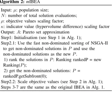
Algorithm 2: mIBEA

Input:µ: population size;

N: number of total solution evaluations;

ρ: objective values scaling factor;

κ: indicator value (hypervolume difference) scaling factor Output:A: Pareto set approximation

Step1: Initialisation (see Step 1 in Alg. 1);

Step2.1: Use the fast non-dominated sorting of NSGA-II to get non-dominated solutions inP and use the non-dominated solutions as the newP.

1) rank the solutions inP: Ranking rankedP = new Ranking(P);

2) get the non-dominated solutions:P = rankedP.getSubfront(0);

Step2.2: Scale objective values (see Step 2 in Alg. 1); Steps 3-7 are the same as the original IBEA in Alg. 1.

IV. COMPUTATIONALRESULTS A. Experimental Design

The following experiments were performed on the full DTLZ problem set (DTLZ1-7) [8]. Our analysis focuses on the three-objective DTLZ1 and 3, as qualitatively good coverage of the true Pareto front can be achieved relatively easily by different algorithms. Besides, these two problems exhibit different properties: DTLZ1 has a planar front in 3D, DTLZ3 has 1/8th of a sphere front in 3D. DTLZ2 and 4 share the same PF as DTLZ3 but differ in the overall domain of the objective values. For example, randomly drawn solutions in the initial population, have objective values of 100-150 in DTLZ1 and 500-1500 in DTLZ3 while the range is significantly smaller e.g., with 2 to 5 in DTLZ2. It is DTLZ1 and 3 where we are expecting the most benefit of the removal of dominated solutions, whereas the insertion of our processing step should be neutral on the other functions.

The settings for the 3D DTLZ problems follow the recom-mended settings from [8]. We are using the algorithms and test functions as implemented in the jMetal framework [10]. For a fair comparison, all algorithms utilise the same operators with the same corresponding parameters. Specifically, a binary tournament selection operator is used for selection. Simulated Binary Crossover (SBX) and polynomial mutation with prob-abilities of 0.9 and (1/number of parameters) respectively, are used to create new offspring. The distribution parameters of the crossover and mutation operators are ηc = 20.0 and ηm= 20.0, respectively. A population size of 100 is used with

the total number of solution evaluations limited to 100,000. Other algorithmic parameters are set as the default settings from the original IBEA [17]. 100 runs of each algorithm are performed. The version of IBEA that we are using for

comparison is the one provided by Brockhoff [4], which has fixed the hypervolume calculation bug in the original IBEA.

In the following, we will assess the performance ofmIBEA qualitatively by inspecting the plots, quantitatively using per-formance indicators and by measuring the runtime. We analyse experimentally the effect that our patch has on IBEA. We do this on DTLZ1-7 and by varying the scaling parameterρand the population sizeµ.

B. Visualisation of Resultant Solution Distributions

The resultant populations under the default setting of

mIBEA, with ρ= 2.0, µ = 100, are illustrated in Figure 2. Compared to the original IBEA presented in Figure 1, the coverage obtained by mIBEA on DTLZ1 and DTLZ3 is a clear improvement. More specifically, the 9890 non-dominated individuals (ndi) found bymIBEA for DTLZ1 spread cross the whole front surface, while the correspondingndifrom IBEA is only 616 and only distributed in the extreme points, resulting in much higher bf (0.9935) than mIBEA (0.5297). Similarly,

mIBEA improves the original IBEA by generating many more non-dominated solutions (ndi= 5292) and solutions between the extreme points (bf = 0.7897) and the central area of the front are found, while the original IBEA only obtains 182 non-dominated solutions which only lie in the corner points.

0 0 0 0.5 0.5 0.5 bf: 0.5297 ndi: 9890 (a)mIBEA on DTLZ1 0 0 0 0.5 0.5 0.5 1 1 1 bf: 0.7897 ndi: 5292 (b)mIBEA on DTLZ3

Fig. 2: Visualisation of the non-dominated solutions found by

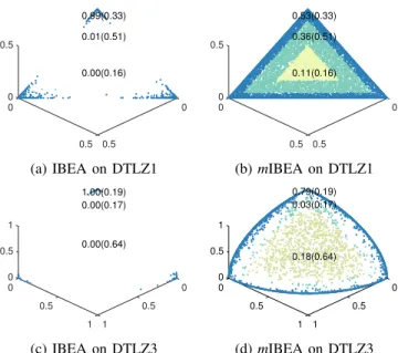
mIBEA on DTLZ1 and DTLZ3 over 100 independent runs. In order to provide more quantitative insights into the distribution of solutions found by each algorithm, Figure 3 compares the proportion of non-dominated solutions found in different regions on each DTLZ problem of the PF. For the three highlighted areas the proportion of the total number of non-dominated solutions contained in the area is provided, with the corresponding proportion of the actual PF surface in 3D the area represents given in the bracket. The boundaries from outermost triangle (blue area) to the innermost triangle (green area) of DTLZ1 are 0.03 and 0.1, for DTLZ3 are 0.1 and 0.2.

For example, in Figure 3b, 0.53(0.33) indicates that the fraction of ndi observed from mIBEA in the blue triangle area of DTLZ1 is 0.53, however the proportion of the total surface this area corresponds to is 0.33. In an ideal solution distribution, the fraction of ndi should be very close to the surface proportion, if one is interested in this coverage notion. Figure 3 also shows thatmIBEA could find new trade-off solutions between extreme points on both DTLZ problems that

(6)

the original IBEA is not able to. In the case of mIBEA, 53% and 79% of non-dominated solutions are found in the edge regions of DTLZ1 and DTLZ3 respectively. Interestingly, a decreased fraction of ndi from the outside to the inside of the PF of DTLZ1 is observed, with a ‘tiny’ fraction (3%) of solutions lie in the middle area (green) area of DTLZ3.

0 0 0 0.00(0.16) 0.5 0.5 0.5 0.01(0.51) 0.99(0.33) (a) IBEA on DTLZ1 0 0 0 0.11(0.16) 0.5 0.5 0.5 0.36(0.51) 0.53(0.33) (b)mIBEA on DTLZ1 0.00(0.64) 0 0 0 0.5 0.5 0.5 0.00(0.17) 1 1 1.00(0.19) 1 (c) IBEA on DTLZ3 0 0 0 0.5 0.5 0.5 1 1 1 0.18(0.64) 0.03(0.17) 0.79(0.19) (d)mIBEA on DTLZ3

Fig. 3: Solution distributions from IBEA and mIBEA on DTLZ1 and DTLZ3

C. A performance analysis of IBEA andmIBEA using different

scaling factor values

In the previous subsection, the objective values scaling factor ρ is fixed to 2.0. As the hypervolume contribution of each solution is calculated based on the scaled objective values (as described in Step2 and Step3 of IBEA, see Section II-A), here we examine the effect of modifying the value ofρ. Within IBEA and mIBEA,ρdirectly affects the ranking of solutions, therefore influencing the preservation of elite solutions.

A series of ρ values within the range of 1.0 to 1024 are tested. From a set of preliminary experiments, we found that when ρ ∈ [1.0,1.1], the PFs on DTLZ functions show no obvious improvement when using either the original IBEA or mIBEA. However whenρ >1.1, some improvement was shown by IBEA and significant improvement by mIBEA. However, when ρ≥ 2, the PFs remain relatively unchanged by both algorithms. Thus, we choose ρ= 1.0,1.15,2.0,64.0

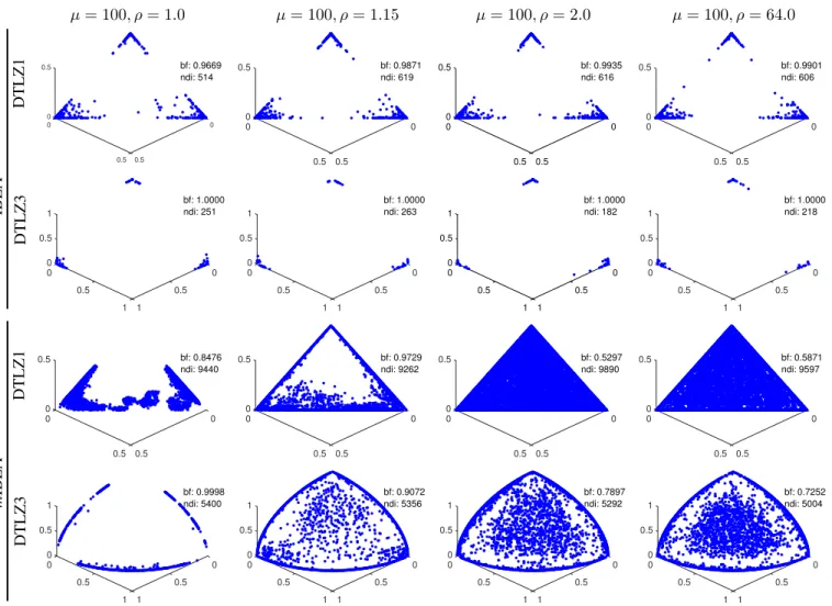
to plot the PFs from IBEA and mIBEA on DTLZ1 and 3 in Figure 4.

As we can see, the scaling parameterρin IBEA has little to no impact on the distribution of the solutions on DTLZ1 and DTLZ3, as the solution sets always collapse to the extreme points of the objective space no matter what the ρ value is. However, ρcan affect the performance ofmIBEA.

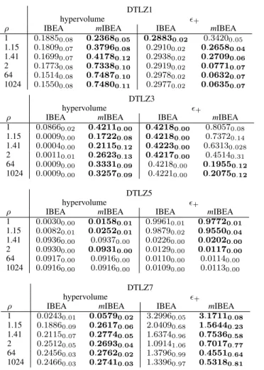
We also compare the performance of IBEA and mIBEA w.r.t. the hypervolume and + indicators across the entire DTLZ family in Table III. The higher hypervolume or lower

+, the better performance of the algorithm has. The reference point of hypervolume is set as 0.5d _{for DTLZ1, where} _d _is

objective index, 1.0d _{for the rest DTLZ problems, DTLZ7}

where the reference point is(1,1,6)due to the third objective. Results that are better with statistical significance (Wilcoxon rank-sum test, 5% significance level) are highlighted in bold. It shows that mIBEA not only improves the coverage of the resultant fronts, but also the convergence, especially on DTLZ1, DTLZ3, and DTLZ7 under all the chosenρ values, as well as mostρvalues of DTLZ6, while performing similarly on DTLZ2, 4 and 5. Only in one of the 14 cases (with standard

ρ= 2), mIBEA is statistically worse, while it is comparable or statistically better in 13 of 14 cases.

In summary, the observations of PF changes from original IBEA andmIBEA suggest the following:

• The original IBEA performs poorly on benchmark func-tions with large objective spaces and comparatively small fronts, i.e. DTLZ1 and DTLZ3 and the change of objec-tive value scaling factor ρ(≥ 1) does not affect (either positively or negatively) the performance;

• Our mIBEA improved IBEA overall on DTLZ1-7 with

wider PF coverage and better convergence w.r.t. hyper-volume and +.

Moreover, the performance comparison between NSGA-II andmIBEA using default settings (µ= 100, ρ= 2) (shown in Table II) suggests thatmIBEA still does not beat NSGA-II on most DTLZ problems. Perhaps it is because the still existing gaps (Fig. 4) and non-uniform solution distribution (Fig. 3) on themIBEA fronts. Further investigations are to be conducted. TABLE II: Performance Comparison of NSGA-II andmIBEA

hypervolume +

NSGA-II mIBEA NSGA-II mIBEA

DTLZ1 0.75720.01 0.73380.10 0.05620.01 0.07710.07 DTLZ2 0.37240.01 0.42170.00 0.12720.02 0.07260.00 DTLZ3 0.37480.01 0.26230.13 0.13150.02 0.45140.31 DTLZ4 0.34720.10 0.28760.14 0.17380.22 0.38630.34 DTLZ5 0.09290.00 0.09310.00 0.01090.00 0.01170.00 DTLZ6 0.08690.01 0.08330.01 0.01800.01 0.02710.01 DTLZ7 0.28180.01 0.26930.04 0.19280.31 0.70170.77

D. A performance analysis of IBEA and mIBEA as the

pop-ulation size changes

We also investigate the performance of both the original IBEA andmIBEA using larger population sizes under different

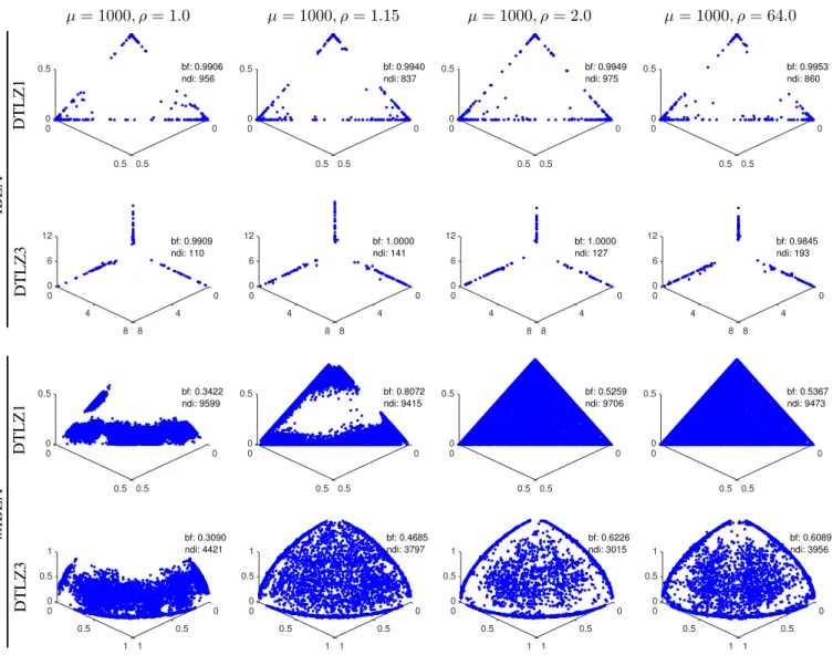
ρ values. Figure 5 shows that when population size goes up to 1000, population size has little affect on PF coverage for DTLZ1 by the original IBEA. It even deteriorates for DTLZ3 on which the maximum of each objective of DTLZ3 is 1.0 on the true PF. However, the proposedmIBEA clearly covers greater parts of the PF surface on both DTLZ1 and DTLZ3 given various ρvalues.

E. Running time of IBEA and mIBEA

As a positive side-effect, the focus on non-dominated so-lutions within mIBEA results in significant speed-ups of the runtime. Table IV shows thatIBEA on average gives an over

(7)

µ= 100, ρ= 1.0 µ= 100, ρ= 1.15 µ= 100, ρ= 2.0 µ= 100, ρ= 64.0 IBEA DTLZ1 0 0 0 0.5 0.5 0.5 bf: 0.9669 ndi: 514 0 0 0 0.5 0.5 0.5 bf: 0.9871 ndi: 619 0 0 0 0.5 0.5 0.5 bf: 0.9935 ndi: 616 0 0 0 0.5 0.5 0.5 bf: 0.9901 ndi: 606 DTLZ3 0 0 0 0.5 0.5 0.5 1 1 1 bf: 1.0000 ndi: 251 0 0 0 0.5 0.5 0.5 1 1 1 bf: 1.0000 ndi: 263 0 0 0 0.5 0.5 0.5 1 1 1 bf: 1.0000 ndi: 182 0 0 0 0.5 0.5 0.5 1 1 1 bf: 1.0000 ndi: 218 m IBEA DTLZ1 0 0 0 0.5 0.5 0.5 bf: 0.8476 ndi: 9440 0 0 0 0.5 0.5 0.5 bf: 0.9729 ndi: 9262 0 0 0 0.5 0.5 0.5 bf: 0.5297 ndi: 9890 0 0 0 0.5 0.5 0.5 bf: 0.5871 ndi: 9597 DTLZ3 0 0 0 0.5 0.5 0.5 1 1 1 bf: 0.9998 ndi: 5400 0 0 0 0.5 0.5 0.5 1 1 1 bf: 0.9072 ndi: 5356 0 0 0 0.5 0.5 0.5 1 1 1 bf: 0.7897 ndi: 5292 0 0 0 0.5 0.5 0.5 1 1 1 bf: 0.7252 ndi: 5004

Fig. 4: PFs of DTLZ1 and DTLZ3 generated by mIBEA with different Rho values (1.0, 1.15, 2.0, and 64). 100 runs are performed for each experiment. The threshold of border fraction (bf) for DTLZ1 is 0.03, and 0.1 for DTLZ3.

8-fold speed-up compared to IBEA using population size of

µ= 1000(theρis set as default value 2.0). The reason is that Step2 in mIBEA (Section III) removes dominated solutions in every generation. Therefore, fewer solutions are persevered in the population, reducing the calculation time for indicator values i.e., hypervolume difference in the original IBEA. As the indicator value calculation is pairwise (Step3 in Section II-A), n2indicator value calculations are required, wherenis the current population size.

V. DISCUSSION AND FUTURE WORK

The proposed mIBEA introduces the ranking from Pareto dominance-based multi-objective evolutionary algorithm into the indicator-based algorithm during the elite solution preser-vation process. The empirical results from mIBEA over the entire DTLZ benchmark functions show that mIBEA signifi-cantly improves the original IBEA on the coverage of resultant Pareto fronts, as well as hypervolume and +. Also, over 8-fold speed-ups are obtained when using a larger population size. Also note that the proposed mIBEA does not introduce any additional parameter to the original IBEA.

However, some gaps are still observable from original IBEA and mIBEA. Similar distributions can be observed from the hypervolume-based SMS-EMOA, although these are better than IBEA. We have performed an initial experiment on the SMS-EMOA’s scaling parameter offset. However, no clear changes have been observed under different offset values. It suggests that the gaps from original IBEA,mIBEA and SMS-EMOA may be a consequence of using the hypervolume as an indicator in optimisation when faces are encountered that are (near-)parallel to at least one objective’s axis.

In the future, we will explore ways to systematically examine the reasons for the gaps and improve mIBEA by redirecting its attention away from extreme solutions, without introducing arbitrary decisions, magic numbers or explicitly defined weights or preferences in the objective space.

ACKNOWLEDGEMENT

This research was supported by the Australian Research Council (DE160100850) and by a Priority Partner Grant by the University of Adelaide, Australia.

(8)

µ= 1000, ρ= 1.0 µ= 1000, ρ= 1.15 µ= 1000, ρ= 2.0 µ= 1000, ρ= 64.0 IBEA DTLZ1 00 0 0.5 0.5 0.5 bf: 0.9906 ndi: 956 0 0 0 0.5 0.5 0.5 bf: 0.9940 ndi: 837 0 0 0 0.5 0.5 0.5 bf: 0.9949 ndi: 975 0 0 0 0.5 0.5 0.5 bf: 0.9953 ndi: 860 DTLZ3 00 0 4 4 6 8 8 12 bf: 0.9909 ndi: 110 0 0 0 4 4 6 8 8 12 bf: 1.0000 ndi: 141 0 0 0 4 4 6 8 8 12 bf: 1.0000 ndi: 127 0 0 0 4 4 6 8 8 12 bf: 0.9845 ndi: 193 m IBEA DTLZ1 00 0 0.5 0.5 0.5 bf: 0.3422 ndi: 9599 0 0 0 0.5 0.5 0.5 bf: 0.8072 ndi: 9415 0 0 0 0.5 0.5 0.5 bf: 0.5259 ndi: 9706 0 0 0 0.5 0.5 0.5 bf: 0.5367 ndi: 9473 DTLZ3 00 0 0.5 0.5 0.5 1 1 1 bf: 0.3090 ndi: 4421 0 0 0 0.5 0.5 0.5 1 1 1 bf: 0.4685 ndi: 3797 0 0 0 0.5 0.5 0.5 1 1 1 bf: 0.6226 ndi: 3015 0 0 0 0.5 0.5 0.5 1 1 1 bf: 0.6089 ndi: 3956

Fig. 5: PFs of DTLZ1 and DTLZ3 generated by IBEA using population size 1000 with different ρ values. 100 runs are performed for each experiment. The threshold of border fraction (bf) for DTLZ1 is 0.03 and DTLZ3 is 0.1.

REFERENCES

[1] T. Back, U. Hammel, and H.-P. Schwefel. Evolutionary computation: Comments on the history and current state.

IEEE Transactions on Evolutionary Computation, 1(1):

3–17, 1997.

[2] N. Beume, B. Naujoks, and M. Emmerich. Sms-emoa: Multiobjective selection based on dominated

hypervol-ume. European Journal of Operational Research, 181

(3):1653–1669, 2007.

[3] K. Bringmann, T. Friedrich, F. Neumann, and M. Wagner. Approximation-guided evolutionary multi-objective opti-mization. InInternational Joint Conference on Artificial

Intelligence (IJCAI), pages 1198–1203. AAAI, 2011.

[4] D. Brockhoff. A bug in the multiobjective optimizer ibea: Salutary lessons for code release and a performance re-assessment. In Int. Conference on Evolutionary

Multi-Criterion Optimization, pages 187–201. Springer, 2015.

[5] S. Chand and M. Wagner. Evolutionary many-objective

optimization: A quick-start guide. Surveys in Operations

Research and Management Science, 20(2):35 – 42, 2015.

[6] C. A. C. Coello, G. B. Lamont, D. A. Van Veldhuizen, et al. Evolutionary algorithms for solving multi-objective

problems, volume 5. Springer, 2007.

[7] K. Deb, A. Pratap, S. Agarwal, and T. Meyarivan. A fast and elitist multiobjective genetic algorithm:

NSGA-II. IEEE Transactions on Evolutionary Computation, 6

(2):182–197, 2002.

[8] K. Deb, L. Thiele, M. Laumanns, and E. Zitzler.Scalable test problems for evolutionary multiobjective optimiza-tion. Springer, 2005.

[9] F. E. C. Duran, C. Cotta, and A. J. Fern´andez-Leiva. A comparative study of multi-objective evolutionary algo-rithms to optimize the selection of investment portfolios with cardinality constraints. In European Conference

on the Applications of Evolutionary Computation, pages

165–173. Springer, 2012.

(9)

TABLE III: The subtables show the hypervolume and the epsilonmeanstd values of IBEA andmIBEA with differentρvalues

but sameµ= 100on DTLZ1-7.

DTLZ1

hypervolume +

ρ IBEA mIBEA IBEA mIBEA

1 0.18850.08 0.23680.05 0.28830.02 0.34200.05 1.15 0.18090.07 0.37960.08 0.29100.02 0.26580.04 1.41 0.16990.07 0.41780.12 0.29380.02 0.27090.06 2 0.17730.08 0.73380.10 0.29190.02 0.07710.07 64 0.15140.08 0.74870.10 0.29780.02 0.06320.07 1024 0.15500.08 0.74800.11 0.29770.02 0.06350.07 DTLZ2 hypervolume +

1 0.02430.01 0.05790.02 3.29960.05 3.17110.08 1.15 0.18860.09 0.26170.06 2.04090.68 1.56440.23 1.41 0.21150.07 0.27740.05 1.63740.96 0.75360.58 2 0.25120.05 0.26930.04 1.09141.06 0.70170.77 64 0.24560.03 0.27620.02 1.37960.99 0.45510.64 1024 0.24660.03 0.27410.03 1.33960.97 0.53180.81

TABLE IV: Average running time comparison (in minutes).

Running Time Comparison (in minutes) µ= 100 µ= 1000 IBEA mIBEA IBEA mIBEA

DTLZ1 0.15 0.08 7.86 1.22 DTLZ2 0.15 0.10 7.62 1.46 DTLZ3 0.15 0.06 8.10 0.24 DTLZ4 0.14 0.11 7.98 1.56 DTLZ5 0.16 0.11 8.01 0.97 DTLZ6 0.15 0.11 8.04 0.21 DTLZ7 0.16 0.10 8.03 1.15

for multi-objective optimization. Advances in

Engineer-ing Software, 42(10):760–771, 2011.

[11] W. Li, E. ¨Ozcan, and R. John. Multi-objective evolution-ary algorithms and hyper-heuristics for wind farm layout optimisation. Renewable Energy, 2016.

[12] T. Tuˇsar and B. Filipiˇc. Differential evolution versus genetic algorithms in multiobjective optimization. In In-ternational Conference on Evolutionary Multi-Criterion

Optimization, pages 257–271. Springer, 2007.

[13] M. Wagner, K. Bringmann, T. Friedrich, and F. Neu-mann. Efficient optimization of many objectives by approximation-guided evolution. European Journal of

Operational Research, 243(2):465 – 479, 2015.

[14] L. Zhao. Performance of Multiobjective Algorithms on

Varying Test Problem Features Using the WFG Toolkit.

PhD thesis, Citeseer, 2007.

[15] A. Zhou, Y. Jin, Q. Zhang, B. Sendhoff, and E. Tsang. Combining model-based and genetics-based offspring generation for multi-objective optimization using a con-vergence criterion. In IEEE Congress on Evolutionary

Computation, pages 892–899. IEEE, 2006.

[16] A. Zhou, B.-Y. Qu, H. Li, S.-Z. Zhao, P. N. Suganthan, and Q. Zhang. Multiobjective evolutionary algorithms: A survey of the state of the art. Swarm and Evolutionary

Computation, 1(1):32–49, 2011.

[17] E. Zitzler and S. K¨unzli. Indicator-based selection in multiobjective search. In International Conference on

Parallel Problem Solving from Nature, pages 832–842.

Springer, 2004.

[18] E. Zitzler, M. Laumanns, L. Thiele, et al. SPEA2: improving the strength pareto evolutionary algorithm, 2001.

[19] E. Zitzler, L. Thiele, M. Laumanns, C. M. Fonseca, and V. G. Da Fonseca. Performance assessment of multiobjective optimizers: an analysis and review. IEEE

Transactions on Evolutionary Computation, 7(2):117–