© 2012 Università del Salento – http://siba-ese.unile.it/index.php/ejasa/index
BAYESIAN ESTIMATION OF POPULATION PROPORTION IN KIM
AND WARDE MIXED RANDOMIZED RESPONSE TECHNIQUE
Zawar Hussain
*(1),(2), Javid Shabbir
(2)(1)Department of Statistics, King Abdulaziz University, Saudi Arabia (2)Department of Statistics, Quaid-i-Azam University, Pakistan
Received 01 May 2011; Accepted 06 January 2012 Available online 14 October 2012
Abstract: In this study, we have developed the Bayesian estimator of the population proportion of a sensitive characteristic when data are obtained through the Randomized Response Technique (RRT) proposed by Kim and Warde [12]. Superiority of the Bayesian estimators is established for a wide range of the values of the population proportion using simple Beta prior information. It is observed that the Bayesian estimators are better than the usual Maximum Likelihood Estimator (MLE) for small as well as moderate samples. The Proposed estimator is also compared with the Warner [29], Kim and Warde [12] and Kim et al. [13] estimators.
Keywords: Bayesian estimation, mean squared error, randomized response technique, simple random sampling.
1.
Introduction
In human population surveys, estimation of population proportion of a stigmatized attribute (induced abortion, drug usage, tax evasion, etc.) with direct questioning method is a complex dealing. An evaluator may possibly collect deceitful answers from the study respondents when he/she uses conventional direct questioning approach. Due to various reasons, information about commonness of stigmatized attributes, in the population, is necessary. Originally, Warner [29] projected an effective method of survey to collect information about stigmatized attributes by providing privacy and secrecy to the respondents. Warner’s procedure consists of two questions A and Ac to be answered on probability foundation. The simple random sampling with replacement (SRSWR) is assumed. The th
i selected respondent is requested to indiscriminately
pick a question (A or Ac) and report yes if his/her real category matches with chosen question
and no otherwise. The probability of a yes for th
i respondent is then given by:
(
)
(
1)(
1)
P yes = =θ pπ+ − p −π (1)
where pis the probability of selecting question A ,and π is population proportion of individuals possessing the stigmatized attribute. The two questions are:
• A= do you belong to possess the sensitive attribute. • Ac= do you not belong to possess the sensitive attribute.
From (1) we get:
(
1)
2 1 p p θ π = − − − . By the method of maximum likelihood, an unbiased estimator of π is:(
)
ˆ 1 1 ˆ , 2 1 2 ML p p p θ π = − − ≠ − , (2) where ˆ n nθ = ʹ′ and nʹ′is the number of yes responses in the sample of n.
The variance of the estimator given in (2) is shown to be:
(
)
(
)
(
)
(
)
2 1 1 ˆ 2 1 ML p p Var n n p π π π = − + − − . (3)A big amount of developments and variants of Warner’s RRT have been suggested by quite a lot of researchers. Greenberg et al. [8], Folsom et al. [7], Christofides [4], Odumade and Singh [20], Mangat [14], Perri [21], Singh and Horn [23], Kim and Warde [12] are some of the many to be cited. The interested readers may be referred to Chaudhuri and Mukerjee [3], Fox and Tracy [6] and Tracy and Mangat [26] for a comprehensive discussion on RRT.
Prior information about the unknown parameter is sometimes obtainable and can be used along with the sample information for estimation of that unknown parameter. This is Bayesian approach of estimation. Hard works done by researchers on Bayesian analysis of randomized response models are not very massive; nonetheless, attempts have been made on the Bayesian analysis of RRTs. Winkler and Franklin [28], Spurrier and Padgett [25], O’Hagan [18], Oh [19], Migon and Tachibana [16], Unnikrishnan and Kunte [27], Barabesi and Marcheselli [1, 2], Hussain et al. [11] and Kim et al. [13] are the major references on the Bayesian analysis of the RRTs.
The arrangement of the paper is as follows. In Section 2, we present the Kim and Warde [12] RRT followed by Bayesian estimation of population proportion and comparisons using Kim and Warde [12] RRT in Section 3. Section 4 contains the conclusions.
2.
Kim and Warde Mixed RRT
To avoid the privacy problems in Moors [17] model, Mangat et al. [15] and Singh et al. [24] proposed alternative models to the Moors model. Specifically, Mangat et al. [15] proposed a random group method which can safeguard the privacy and anonymity of the respondents but it has an efficiency problem. Singh et al. [24] proposed models assumed simple random sampling without replacement which led to a high-cost survey compared with the Moors [17] model using simple random sampling with replacement. To circumvent these drawbacks of Mangat et al. [15] and Singh et al. [24] models, Kim and Warde [12] proposed a new randomized response model using simple random sampling. In Kim and Warde [12] RRM, each sample respondent, selected by simple random sampling with replacement, is asked to answer a direct question “I am a member of innocuous trait group”. If a respondent answers yes, then he/she is directed to go to randomization device R1 consisting of two statements (i) “I am a member of the sensitive trait group” and (ii) I am a member of innocuous trait group with pre-assigned probabilities T1 and (1-T1). If a respondent answers no to the direct question, then the respondent is requested to use randomization device R2 consisting of the statements of the Warner [29] RRT with pre-assigned probabilities p and (1- p) respectively. The proportion of yes responses from the respondents using R1 is given by:
(
)
(
)
1 1 1 I 1 1 1
T T T T
ψ = π+ − π = π + − , (4)
where πI is proportion of individuals possessing innocuous trait. An estimator of π is defined
as:
(
1)
1 ˆ 1 ˆa T T ψ π = − − .The variance of πˆa is given by:
( )
(
2) (
)
1(
1)
1 1 1 1 1 1 1 ˆa T T Var n T n T π π ψ ψ π = − = − ⎡⎣ + − ⎤⎦.The proportion of yes answers from the respondents using R2is given by (1). Another unbiased estimator of πis given by (2) with variance given by (3).
KM 1 2 1 ˆ n ˆa n ˆ for 0<ML n 1 n n n π = π + π < . The choice 1 1 2 p T =
− provides equal privacy protection in both the randomization
devicesR1andR2. With this choice, variance of the estimator ˆKM
π is given by:
(
KM)
(
) (
1)
1(
) (
)
2 1 1 1 1 1 ˆ T T Var n nT λ π π π π π = − + − ⎡⎣ − + − ⎤⎦, for n n= 1+n2 and n1 nλ= , where n1 and n2 are the numbers of yes responses from the
respondents using R1 and R2 respectively. The two problems with ˆKM
π are apparent (i) the
estimator may assume values outside the interval [0,1] and (ii) the variance of the estimator depends upon the numbers (n1andn2) of respondents using randomization devices R1 and R2.
3.
Bayesian Estimation of using Kim and Warde (2005) RRT and
Comparisons
In many practical situations where we have some uncertainty about our parameter of interest (π) which is formally given in the form of prior distribution (see Winkler and Franklin [28], and Spurrier and Padgett [25]), we use Beta distribution as a prior density for π which is quite natural and common choice in literature (see Barabesi and Marcheselli [1] and Hussain and Shabbir [9, 10]). The probability model for the π in the form of Beta distribution with α and
βas hyperparameters is given as:
(
,)
(
1)
1(
1)
1 , 0 1. Beta , f α β π α β π π π α β − − = − ≤ ≤Now we develop a Bayesian analysis of Kim and Warde [12] RRT assuming a simple random sample with replacement (SRRWR). A sample of size n individuals is drawn and Kim and Warde [12] RRT is applied to collect responses from the selected individuals. Also we assume that the number of respondents in each of the sub sample is known by some way.
Let 1 1 n i i X Y =
=
∑
be the number of yes responses from the respondents using R1, where Yi is aBernoulli random variable with probability of a yes given by (4). Now the conditional distribution of X given π is:
(
)
(
)
(
) (
)
1 1 / 1 1 1 1 1 ! / 1 1 1 ! ! x n x X n f x T T T T x n x π π π π − = + − − − + −(
)
(
) (
)
1 1 1 1 1 ! 1 ! ! x n x n n T d x n x π π − = + − −(
)
(
)
(
)
1 1 1 1 0 1 ! ! 1 ! ! ! ! x n x n x j j j n x T d x n x π j x j π − − = = − −∑
− , (5) for(
1)
1 1 1 0,1, 2..., , where T x n d T −= = . The last step in (5) follows by simply writing
(
π +d)
xinits binomial expansion. Thus, the posterior distribution of π given X is:
(
)
(
)
(
)
(
)
(
)
(
)
1 1 1 0 / 1 0 ! 1 ! ! / 0 1 . ! , ! ! x n x x j j j X x x j j x d j x j f x I x d j n x j x j β α π π π π β α β + − − − + − = Π − = − − = < < + + − −∑
∑
Assuming a squared error loss function a closed form expression of the Bayesian estimator from the responses of the respondents using R1, is given by:
(
)
(
)
(
)
(
)
1 1 1 1 1 0 0 1 0 ! 1 ! ! ˆ . ! , ! ! x n x x j j j B x x j j x d d j x j x d j n x j x j β α π π π π β α β + − − − + − = − = − − = + + − −∑
∫
∑
or(
)
(
)
(
)
(
)
1 1 0 1 0 ! 1, ! ! ˆ ! , ! ! x x j j B x x j j x d j n x j x j x d j n x j x j β α β π β α β − = − = + + + − − = + + − −∑
∑
. (6) Let 2 1 n i i T W ==
∑
be number of yes responses from the respondents usingR2, where Wi =1 withprobability θ and Wi =0 with probability
(
1−θ
)
, where θ is defined as in (1). The conditional(
)
(
)
(
(
)(
)
)
(
(
)(
)
)
2 2 / 2 ! / 1 1 1 1 1 ! ! t n t T n f t p p p p t n t π π π π π π − = + − − − − − − −(
)
(
) (
) (
)
2 2 2 2 ! 2 1 1 ! ! n t n t n p g g t n t π π − = − + − + −(
)
(
)
(
)
(
)
(
)
(
)
2 2 2 2 0 0 2 2 ! ! ! 2 1 1 ! ! ! ! ! ! n t t n n j i i j i j n t n t p g t n t i t i j n t j π π − − − = = − = − − −∑ ∑
− − − , (7) for(
)
(
)
2 1 0,1, 2..., , where 2 1 p t n g p − = = − .Thus, the posterior distribution of π given T is:
(
)
(
)
(
)
(
)
(
)
2 2 1 2 1 / 0 0 2 ! ! / 1 ! ! ! ! n t t j n j i i T i j n t t f t k g i t i j n t j β α π π π − + − − − +− Π = = − = − − − −∑ ∑
, where(
)
(
)
(
)
(
)
2 2 0 0 2 1 ! ! , ! ! ! ! n t t n j i i j k n t t g i j i t i j n t j β α β − − − = = = − + + − − −∑ ∑
.Under the squared error loss function a closed form expression of the Bayesian estimator of
πbased on the responses form the respondents using R2 is given by:
(
)
(
)
(
)
(
)
(
)
(
)
(
)
(
)
2 2 2 2 2 1 1 1 1 2 0 0 2 0 2 0 0 2 ! ! 1 ! ! ! ! ˆ ! ! , ! ! ! ! n t t j n j i i i j B t n t n j i i j n t t g d i t i j n t j n t t g i j i t i j n t j β α π π π π β α β − + − − − + +− = = − − − = = − − − − − = − + + − − −∑ ∑
∫
∑ ∑
or(
)
(
)
(
)
(
)
(
)
(
)
(
)
(
)
2 2 2 2 2 2 0 0 2 2 0 0 2 ! ! 1, ! ! ! ! ˆ ! ! , ! ! ! ! n t t n j i i j B t n t n j i i j n t t g i j i t i j n t j n t t g i j i t i j n t j β α β π β α β − − − = = − − − = = − + + + − − − = − + + − − −∑ ∑
∑ ∑
. (8)Now using (6) and (8), we may define the Bayesian estimator of πas:
1 2
Prop 1 2
ˆ n ˆB n ˆB
n n
Before moving towards formal comparisons of different estimators under study, we point out some computational issues related to our study. From (6), (8) and (9) it is apparent that the Bayesian estimator involves a large computation especially when the sample size and/or the number of yes responses is large. To deal with this difficulty we have written a program in R software (this program is available with the first author). As from the expression of the Bayesian estimator it is clear that it cannot be written as a linear function of the usual MLE, therefore, the approach of Samaneigo and Reneau [22] of using Bayes relative risk relative to an unknown true prior distribution for making comparison of Bayesian and Classical point estimators cannot be applied here. Chaubey and Li [5] used Classical approach to compare the Bayesian and Classical estimators and did not use a loss function. The same approach of comparison is used by Kim et al. [13] and we also follow the same approach in our study.
As it is obvious that the two estimators πˆa and πˆML(and πˆB1 and
2
ˆB
π ) are dependent. Moreover,
unbiasedness property is not associated with
1
ˆB
π and πˆB2. Therefor, to take care of biasedness
and dependence issue we define the approximate Mean Squared Errors (MSEs) of the Bayesian ( ˆProp
π ) and classical estimator (πˆKM), for a fixed value of π, as:
(
)
( )
(
)
2 2
KM 1 2
ˆ n ˆa n ˆML
MSE MSE MSE
n n π ≈⎛⎜ ⎞⎟ π +⎛⎜ ⎞⎟ π ⎝ ⎠ ⎝ ⎠ , and
(
)
( )
1( )
2 2 2 Pr op 1 2 ˆ n ˆB n ˆBMSE MSE MSE
n n π ≈⎛⎜ ⎞⎟ π +⎛⎜ ⎞⎟ π ⎝ ⎠ ⎝ ⎠ , where
( )
ˆa(
ˆa)
2 MSE π =E π −π(
)
(
)
(
)
1 1 2 1 0 1 ! ˆ 1 ! ! n n x x a x n x n x π π ψ ψ − = = − − −∑
(
ˆML)
(
ˆML)
2 MSE π =E π −π(
)
(
)
( ) (
)
2 2 2 2 0 2 ! ˆ 1 ! ! n t n t ML t n t n t π π θ θ − = = − − −∑
( )
1(
1)
2 ˆB ˆB MSEπ
=Eπ
−π
(
)
(
)
(
)
1 1 1 2 1 0 1 ! ˆ 1 ! ! n n x x B x n x n x π π ψ ψ − = = − − −∑
( )
2(
2)
2 ˆB ˆB MSE π =E π −π(
)
(
)
( ) (
)
2 2 2 2 2 0 2 ! ˆ 1 ! ! n t n t B t n t n t π π θ θ − = = − − −∑
Using the Mangat [14] RRT, Kim et al. [13] proposed a Bayesian estimator which can be compared with proposed Bayesian estimator. Kim et al. [13] estimator ˆBK
(
)
(
)
(
)
(
)
0 BK 0 ! 1, ! ! ˆ ! , ! ! x x j j x x j j x h j n x j x j x h j n x j x j β α β π β α β − = − = + + + − − = + + − −∑
∑
,h 1 p p − = .The MSE ofthe Kim et al. [13] estimator ˆBK
π is given by:
(
BK)
(
BK)
2(
BK)
2(
)
0 ˆ ˆ n ˆ x 1 n x x MSE π E π π π π φ φ − = = − =∑
− − ,where φ= pπ+
(
1−p)
. Also, when data are obtained by Warner [29] RRT with probability of ayes answer given by (4), the Bayes estimator of the population proportion πis given by:
(
)
(
)
(
)
(
)
(
)
(
)
(
)
(
)
0 0 W 0 0 ! ! 1, ! ! ! ! ˆ ! ! , ! ! ! ! t n t n j i i j t n t n j i i j n t t g a i b j i t i j n t j n t t g a i b j i t i j n t j β π β − − − = = − − − = = − + + + − − − = − + + − − −∑∑
∑∑
.Its MSE is given by:
( )
ˆW(
ˆW)
2 MSE π =E π −π(
)
(
)
( ) (
)
2 W 0 ! ˆ 1 ! ! n t n t t n t n t π π θ θ − = = − − −∑
.For comparison purposes, we have chosen a Beta prior with mean equal to 0.05 (i.e.
α/(α+β)=0.05) for both the subsamples of the respondents using R1 and R2. Figures 1- 5 demonstrate the behavior of the MSEs of the estimators ˆPr op
π ,πˆKM, πˆBKand πˆW. This shows the
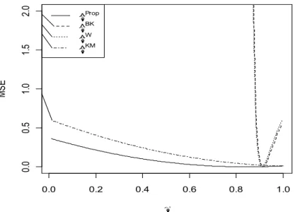
robustness of Bayes estimators against the misspecification of prior distribution. From the Figures 1-5, we can observe that MSE of the proposed Bayesian estimator is less than the other competitor estimators over a wide range of π and is not much affected by changing T1. It has also been noted that the performance of the proposed estimator remains better no matter how many respondents used the randomization device R1or R2. For Instance, in Figure 5, n1=5
andn2 =20contrary to the case of Figure 1 where n1 =15,n2 =10. Moreover, the relative
efficiency of the proposed Bayesian estimator decreases (as expected) as π moves from 0 to 1. Better performance of the proposed Bayesian estimator for large values of πdepicts an important point that even in the case of misspecified prior distribution proposed Bayesian estimator performs better than the other estimators discussed in this article. This study shows that Kim and Warde [12] RRT should be used to gather the data and Bayesian estimation should be applied. For large samples, we have observed that relative efficiency of the proposed estimator decreases. This suggests using the proposed Bayesian estimation in a stratified random sampling protocol which could be a subject of the future studies.
0.0 0.2 0.4 0.6 0.8 1.0 0. 0 0. 5 1. 0 1. 5 2. 0 p MS E p^Prop p^ BK p^W p^KM
Figure 1. MSEs of πˆProp,πKM,πˆBK,πˆWfor n1=15,n2 =10T1=0.6,α =1,β =19 and π ranging from 0 to 1. 0.0 0.2 0.4 0.6 0.8 1.0 0. 0 0. 5 1. 0 1. 5 2. 0 p MS E p^ Prop p^ BK p^ W p^ KM
Figure 2, MSEs of πˆProp,πKM,πˆBK,πˆWfor n1=15,n2 =10T1 =0.7,α =1,β =19 and π ranging from 0 to 1.
0.0 0.2 0.4 0.6 0.8 1.0 0. 0 0. 5 1. 0 1. 5 2. 0 p MS E p^ Prop p^ BK p^ W p^ KM
Figure 3. MSEs of πˆProp,πKM,πˆBK,πˆWfor n1=15,n2 =10T1=0.8,α =1,β =19 and π ranging from 0 to 1. 0.0 0.2 0.4 0.6 0.8 1.0 0. 0 0. 5 1. 0 1. 5 2. 0 p MS E p^ Prop p^ BK p^ W p^ KM
Figure 4. MSEs of πˆProp,πKM,πˆBK,πˆWfor n1=15,n2 =10T1=0.9,α =1,β =19 and π ranging from 0 to 1.
0.0 0.2 0.4 0.6 0.8 1.0 0. 0 0. 5 1. 0 1. 5 2. 0 p MS E p^ Prop p^ BK p^ W p^ KM
Figure 5. MSEs of πˆProp,πKM,πˆBK,πˆWfor n1 =5,n2 =20T1=0.6,α =1,β =19 and π ranging from 0 to 1.
5.
Conclusions
We have presented the Bayesian estimation of the population proportion when the data are gathered through the Kim and Warde [12] RRT. Using a simple prior distribution, we have presented the graphs for some selected values of the design parameters and population proportion. We observed that when sample size is small, the proposed Bayesian estimators, even with misspecified prior information, perform better than the MLE and the Warner [29] and Kim et al. [13] Bayes estimators. Moreover, the performance of proposed estimator does not depend upon the number of respondents using either R1orR2. The proposed Bayesian estimator is bound to lie in [0,1]but this may not be case with Kim and Warde [12] likelihood estimator. Overall we may conclude the better performance of proposed estimator over that of Kim and Warde [12] MLE and Bayesian estimators based on Warner [29] and Kim et al. [13] RRTs.
References
[1]. Barabesi, L., Marcheselli, M. (2006). A practical implementation and Bayesian estimation in Franklin’s randomized response procedure. Communication in Statistics- Simulation and Computation, 35, 365-573.
[2]. Barabesi, L., Marcheselli, M. (2010). Bayesian estimation of proportion and sensitivity level in randomized response procedures. Metrika, 72, 75-88.
[3]. Chaudhuri, A., Mukerjee, R. (1988). Randomized response: Theory and Methods. New York: Marcel- Decker,.
[4]. Christofides, T. C. (2003). A generalized randomized response technique. Metrika, 57, 195-200.
[5]. Chaubey, Y., Li, W. (1995). Comparison between maximum likelihood and Bayes methods of estimation for binomial probability with sample compositing. Journal of Official Statistics, 11, 379-390.
[6]. Fox, J., Tracy, P. (1986). Randomized response: Theory and techniques, Marcel-Dekker, New York.
[7]. Folsom, R. E., Greenberg, B. G., Horvitz, D. G., Abernathy, J. R. (1973). The two alternate question randomized response model for human surveys. Journal of the American Statistical Association, 68, 525-530.
[8]. Greenberg, B., Abul-Ela, A., Simmons, W., Horvitz, D. (1969). The unrelated question randomized response: theoretical framework. Journal of the American Statistical Association, 64, 529-539.
[9]. Hussain, Z., Shabbir, J. (2009a). Bayesian estimation of population proportion of a sensitive characteristic using simple Beta prior. Pakistan Journal of Statistics, 25(1), 27-35.
[10]. Hussain, Z., Shabbir, J. (2009b). Bayesian Estimation of population proportion in Kim and Warde (2005) Mixed Randomized Response using Mixed Prior Distribution. Journal of probability and Statistical Sciences, 7(1), 71-80.
[11]. Hussain, Z. Shabbir, J., Riaz, M. (2011). Bayesian Estimation Using Warner’s randomized Response Model Through Simple and Mixture Prior Distributions. Communications in Statistics- Simulation and Computation, 40(1), 159-176.
[12]. Kim, J. M., Warde, D. W. (2005). A mixed randomized response model. Journal of Statistical Planning and Inference, 133(1), 211-221.
[13]. Kim, J. M., Tebbs, J. M., An, S. W. (2006). Extension of Mangat’s randomized response model. Journal of Statistical Planning and Inference, 36(4), 1554-1567.
[14]. Mangat, N. S. (1994). An improved randomized response strategy. Journal of the Royal Statistical Society, B, 56(1), 93-95.
[15]. Mangat, N.S., Singh, R., Singh, S. (1997). Violation of respondent's privacy in Moors' model—its rectification through a random group strategy response model. Communications in Statistics- Theory and Methods, 26 (3), 243–255.
[16]. Migon, H., Tachibana, V. (1997). Bayesian approximations in randomized response models. Computational Statistics and Data Analysis, 24, 401-409.
[17]. Moors, J. J. A. (1971). Optimizing of the unrelated question randomized response model. Journal of the American Statistical Association, 66, 627-629.
[18]. O’Hagan, A. (1987). Bayes linear estimators for randomized response models. Journal of the American Statistical Association, 82, 580-585.
[19]. Oh, M. (1994). Bayesian analysis of randomized response models: a Gibbs sampling approach. Journal of the Korean Statistical Society, 23, 463-482.
[20]. Odumade, O., Singh, S. (2009). Improved Bar-Lev, Bobovich, and Boukai randomized response Models. Communication in Statistics-Simulation and Computation, 38(3), 473-475.
[21]. Perri, P. F. (2008). Modified randomized devices for Simmons’ model. Model Assisted Statistics and Applications, 3, 233-239.
[22]. Samaneigo, F., Reneau, D. (1994). Towards a reconciliation of the Bayesian and frequentist approaches to the point estimation. Journal of the American Statistical Association, 89, 947-957.
[23]. Singh, S., Horn, S. (1998). Estimation of stigmatized characteristics of a hidden gang in finite population. Australian and New Zealand Journal of Statistics, 40(3), 291-297.
[24]. Singh, S., Singh, R., Mangat, N.S. (2000). Some alternative strategies to Moors' model in randomized response model, Journal of Statistical Planning and Inference, 83, 243–255. [25]. Spurrier, J., Padgett, W. (1980). The application of Bayesian techniques in randomized
response. Sociological Methodology, 11, 533-544.
[26]. Tracy, D., Mangat, N. (1996). Some development in randomized response sampling during the last decade-a follow up of review by Chaudhuri and Mukerjee. Journal of Applied Statistical Science, 4, 533-544.
[27]. Unnikrishnan, N., Kunte, S. (1999). Bayesian analysis for randomized response models. Sankhya, B, 61, 422-432.
[28]. Winkler, R., Franklin, L. (1979). Warner’s randomized response model: A Bayesian approach. Journal of the American Statistical Association, 74, 207-214.
[29]. Warner, S. L. (1965). Randomized response: a survey technique for eliminating evasive answer bias. Journal of the American Statistical Association, 60, 63-69.
This paper is an open access article distributed under the terms and conditions of the Creative Commons Attribuzione - Non commerciale - Non opere derivate 3.0 Italia License.