1 2 3 4 5 6 7 8 9 10 11 12 13 14 15 16 17 18 19 20 21 22 23 24 25 26 27 28 29 30 31 32 33 34 35 36 37 38 39 40 41 42 43 44 45 46 47 48 49 50 51 52 53 54 55 56 57 58 59 60 61 62 63
Evaluation of ECMWF medium-range ensemble forecasts
of precipitation for river basins
J. Ye,
a,b* Y. He,
cF. Pappenberger,
d,aH. L. Cloke,
e,fD. Y. Manful
gand Z. Li
aaCollege of Hydrology and Water Resources, Hohai University, Nanjing, China AQ bHuai River Basin Meteorological Centre, Bengbu, China
cTyndall Centre for Climate Change Research, School of Environmental Sciences, University of East Anglia, Norwich, UK dEuropean Centre for Medium-Range Weather Forecasts, Reading, UK
eDepartment of Geography and Environmental Science, University of Reading, UK fDepartment of Meteorology, University of Reading, UK
gInstitute for Landscape Ecology and Resources Management, University of Giessen, Germany
*Correspondence to: J. Ye. E-mail: [email protected] AQ2
Providing probabilistic forecasts using Ensemble Prediction Systems has become
increasingly popular in both the meteorological and hydrological communities. Compared
to conventional deterministic forecasts, probabilistic forecasts may provide more reliable
forecasts of a few hours to a number of days ahead, and hence are regarded as better
tools for taking uncertainties into consideration and hedging against weather risks. It is
essential to evaluate performance of raw ensemble forecasts and their potential values in
forecasting extreme hydro-meteorological events. This study evaluates ECMWF’s
medium-range ensemble forecasts of precipitation over the period 1 January 2008 to 30 September
2012 on a selected midlatitude large-scale river basin, the Huai river basin (
ca
. 270 000 km
2)
in central-east China. The evaluation unit is sub-basin in order to consider forecast
performance in a hydrologically relevant way. The study finds that forecast performance
varies with sub-basin properties, between flooding and non-flooding seasons, and with the
forecast properties of aggregated time steps and lead times. Although the study does not
evaluate any hydrological applications of the ensemble precipitation forecasts, its results
have direct implications in hydrological forecasts should these ensemble precipitation
forecasts be employed in hydrology.
Key Words: ECMWF EPS; Huai; skill score; diurnal cycle
Received 24 March 2013; Revised 4 July 2013; Accepted 16 August 2013; Published online in Wiley Online Library
1. Introduction
A deterministic weather forecast is a single model trajectory generated by a numerical weather prediction (NWP) system. It is highly dependent on the estimation of the initial atmospheric conditions and does not take uncertainties into consideration. If the initial conditions are incorrect, the forecast will fail to replicate weather events correctly. Since the inherent stochastic nature of a weather system was discussed by Lorenz (1963, 1969), it has been recognised that a perfect numerical weather forecast is unattainable (Hamillet al., 2000) because a tiny error in the initial conditions will grow inevitably and a deterministic forecast is ‘determined’ to fail. An alternative approach is to incorporate uncertainties by finding reasonable probabilistic distribution functions of atmospheric conditions and generating multiple forecasts from different initial conditions, and sometimes from different model parametrizations. Leith (1974) called such forecasts ‘Monte Carlo Forecasts’, now usually referred to as an Ensemble Prediction System (EPS). Leith (1974) suggests the mean of a forecast ensemble is the estimate of the true state
of the atmosphere that is best in the least-square-error sense. Buizza (2008) interprets EPS as a system based on a finite number of deterministic integrations and the only feasible method in meteorology to predict a probability density function beyond the range of linear error growth. EPS has been embraced by the meteorological community as a practical way of estimating uncertainties of a weather forecast (Hamillet al., 2000). It has also become popular in the field of hydrology and water resources management (Thielenet al., 2008), which has been demonstrated by the Hydrologic Ensemble Prediction EXperiment (HEPEX) (for a comprehensive review see Cloke and Pappenberger (2009) and visit www.hepex.org) for a wide range of water-related hazards (Alfieriet al., 2012).
The performance of EPS has been constantly assessed by meteorologists and more recently by hydrologists using a variety of ensemble verification statistics such as the Brier score (BS), the ranked probability score (RPS), the relative operating characteristic (ROC) and others (see e.g. Cloke and Pappenberger, 2008). Meteorologists usually compute the statistics of variables that may not be directly relevant for hydrology, e.g. geopotential
c
1 2 3 4 5 6 7 8 9 10 11 12 13 14 15 16 17 18 19 20 21 22 23 24 25 26 27 28 29 30 31 32 33 34 35 36 37 38 39 40 41 42 43 44 45 46 47 48 49 50 51 52 53 54 55 56 57 58 59 60 61 62 63 64 1 2 3 4 5 6 7 8 9 10 11 12 13 14 15 16 17 18 19 20 21 22 23 24 25 26 27 28 29 30 31 32 33 34 35 36 37 38 39 40 41 42 43 44 45 46 47 48 49 50 51 52 53 54 55 56 57 58 59 60 61 62 63 64 height at 500 hPa (Molteni et al., 1996), or may not have the
appropriate spatial scales for hydrological models, e.g. average precipitation over grids (Buizza, 1999). Readers can also see AQ3
discussion in Pappenbergeret al.(2008a) and Pappenberger and Buizza (2009). It is therefore difficult to draw conclusions on the efficacy of EPS when applied in the field of hydrology and other associated fields resulting often in the development of novel scores reflecting the needs of a particular community (Pappenberger
et al., 2011a). Most studies of hydro-meteorological forecast systems include not only an evaluation of forecast hydrological forecast skill but also meteorological skill (e.g. Pappenberger
et al., 2005, 2011b; De Rooet al., 2011; Voisinet al., 2011). There are a number of studies that assess the ‘hydrological’ quality of EPS by focusing on the performance of ensemble forecasts of precipitation and the simulated ensemble discharge. For example, Thirelet al.(2008) assess the quality of the European Centre for Medium-range Weather Forecasts (ECMWF) and M´et´eo-France Pr´evision d’Ensemble ARPEGE (PEARP) EPS precipitation over France using the Brier skill score (BSS) and the ranked probability skill score (RPSS). Vel´azquez et al.(2009) used Continuous Ranked Probability Score (CRPS) and the rank histogram for evaluating a Canadian hydrological ensemble prediction system (H-EPS). Heet al.(2009) evaluated the performance of ensemble precipitation and discharge forecasts of January 2008 from seven forecast centres for the Upper Severn catchment using CRPS and ROC. Such studies are valuable in facilitating hydrological applications of EPS. But they do not necessarily provide detailed analysis of the ensemble precipitation, e.g. the performance at different time steps (in particular sub-daily time steps), lead times or for river basins with various properties, and most of them only study a number of individual events or seasons.
Ensemble forecasts have yet to be used to their full potential, although they have been produced for nearly two decades. One of the main reasons is that their performance is often deemed to be too poor to provide ‘harmless’ operational forecasts. Their uncertainties are considerably large especially as the lead times increase. False alarms do not only cost significantly in financial terms but also damage the reputation of forecasting institutions. Operational forecasters often have to make a binary decision whether or not an action should be taken. It is not so straightforward for decision makers to utilise ensemble forecasts in terms of probabilities compared to conventional deterministic forecasts whereby a binary decision can be made based on a single forecast, albeit with inevitable errors in the single forecast. This is often the second ‘excuse’ for ignoring ensemble forecasts. Readers can refer to Demerittet al.(2010) for more detailed discussion on challenges in communicating and using ensembles in operational flood forecasting. This article aims to address the first question: how poor or how good the forecasts are, based on the current generation of model and data assimilation methods.
ECMWF has been producing short to medium range (0–15 days forecast lead time) ensemble weather forecasts operationally since November 1992. Such weather forecasts have also been produced at a number of other centres, along with ECMWF, which have recently shared products and emerged into the so-called TIGGE initiative, acronym for THORPEX Interactive Grand Global Ensemble (Bougeaultet al., 2010), which has been used in many hydrometeorological forecasting studies (e.g. Pappenberger et al., 2008b; He et al., 2009). This article focuses on ECMWF’s ensemble forecasts only, but its methods can be applied to study other ensemble prediction systems.
The Huai river basin is selected in this study because it has a good-quality precipitation observational dataset. It is located in midlatitudes straddling the southern monsoon and the northern continental climate, which makes the basin an interesting and challenging test bed. The basin encompasses one of the fastest growing economic regions in China but is highly vulnerable to extreme hydrometeorological events, with floods as the worst disaster in this basin. Its average population density isca. 600 km−2 (Ninget al., 2003), more than four times the national average of
138 km−2. Major basin-wide floods have been recorded once every 5 years on the average and local floods once every 2 or 3 years (Huai River Commission, Ministry of Water Resources, 2010) and affect millions of people. The period between May and September is officially regarded as the basin’s flooding season, although large spring floods have occurred in April a number of times in past years. Snowfall is rare and thus large floods are mainly driven by heavy rainfall. Due to the significant economic value of the basin and its frequent devastating floods, a number of recent studies have pointed to the potential of using ensemble forecasts in this basin. Heet al.(2010) use six forecast centres from the TIGGE archive to drive a coupled atmospheric–hydrologic cascade system to hindcast three 2007 flood events on the Upper Huai sub-basin (30 672 km2). The results demonstrate that the TIGGE multi-model ensemble has great potential to produce skilful forecasts of river discharge and improve the warning time to as early as 10 days in advance. Yang
et al.(2012) use generalised additive models and Bayesian model averaging (BMA) to post-process the ensemble forecasts from the National Centers for Environmental Prediction (NCEP).The method was applied to the Yishusi river sub-basins, in the eastern part of the Huai river basin, for July 2007. The BMA forecasts outperform the raw ensemble forecasts especially for extreme precipitation. Liuet al.(2013) evaluate the forecasting skills of post-processed ensemble forecasts from a fixed version of the Global Forecast System (GFS) produced by NCEP. Their study is carried out for 15 sub-areas of the Huai river basin for 23 years starting from 1981. The post-processing method applied in their study can remove all the biases in the raw ensemble forecasts, and improve the forecasting skill and ensemble spread.
The above-mentioned studies however did not carry out detailed analysis of the performance of the raw ensemble forecasts which is the basis of both precipitation post-processing and further application in hydrology and other fields. This was partly due to the fact that a homogenised precipitation database for the entire basin was not readily available to enable a rigorous performance evaluation of the raw forecasts. Br¨ocker (2012) points out that performance evaluation of raw ensembles may serve as a benchmark for more sophisticated ensemble interpretation models. The availability of hourly observed precipitation analysis at high spatial resolution produced by the China Meteorological Administration (CMA) has provided a perfect opportunity to evaluate ensemble forecasts near real time and at sub-daily resolutions.
This article aims to carry out an in-depth assessment of ECMWF’s medium-range ensemble precipitation forecasts and address three scientific questions: (i) how skilful are ECMWF’s ensemble forecasts over this midlatitude river basin; (ii) how do the forecast skills vary with seasons, sub-basin properties, lead times and aggregated time steps; and (iii) do sub-daily ensemble forecasts bring any benefits or are they simply unwanted noise generated by the current model version? The article is organised in the following way. The study area and data are described in section 2. The experimental design and scores used for evaluation are explained in section 3. The results are presented and discussed in section 4, which is followed by the final concluding section.
2. Study area and data description 2.1. The Huai river basin
The Huai river basin is located in central east China, between the lower reaches of the Yellow and the Changjiang (Yangtze) Rivers (112–121◦N, 31–36◦E). It has a total drainage area of approximately 270 000 km2 (Figure 1). It consists of two river systems, namely the Huai rivers and the Yishusi rivers. The Huai originates from the Tongbai Mountains in Henan province, flows towards the east through Henan, Anhui and Jiangsu provinces. The total length of the Huai’s main reach is over 1000 km with
1 2 3 4 5 6 7 8 9 10 11 12 13 14 15 16 17 18 19 20 21 22 23 24 25 26 27 28 29 30 31 32 33 34 35 36 37 38 39 40 41 42 43 44 45 46 47 48 49 50 51 52 53 54 55 56 57 58 59 60 61 62 63 64 1 2 3 4 5 6 7 8 9 10 11 12 13 14 15 16 17 18 19 20 21 22 23 24 25 26 27 28 29 30 31 32 33 34 35 36 37 38 39 40 41 42 43 44 45 46 47 48 49 50 51 52 53 54 55 56 57 58 59 60 61 62 63 64 Color F igure -P rint and O nline
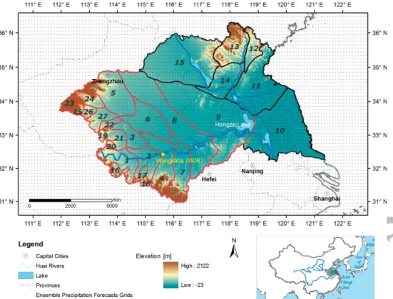
Figure 1.Elevation map of 27 Huai sub-basins (refer to Table 1 for their characteristics) located in central east China. The location is indicated in the right lower panel with blue lines representing the Yellow and Changjiang rivers. Sub-basins nos. 10–15 belong to the Yishusi rivers and the remaining belong to the Huai rivers.
an average elevation drop of 200 m, of which 178 m of the drop is up to the Wangjiaba (WJB) sluice gate, 22 m up to Hongze Lake. The relatively low elevation drop in the middle and lower reaches (22 m) leads to flattened flow velocity and increased risk of over-bank flow and inundation. To the northeast side of the basin is the Yishusi river system, most of which is on the former Yellow river flood plain as a product of ancient Yellow river floods and resulting river path alterations. The Yishusi originates from the Yimeng Mountains in Shandong province and mostly flows through Shandong and Jiangsu provinces and joins the Hongze Lake in the south. It has over 15 tributaries or channels that empty into the Yellow Sea. The entire basin is divided into 27 sub-basins, merging two sub-basin boundary definitions used by the Huai Basin Meteorological Centre and the Huai River Commission. Sub-basins nos. 10–15 belong to the Yishusi and the remaining to the Huai. Due to thousands of existing hydraulic structures in the basin, its sub-basin delineation cannot solely depend on the natural topography and elevation. Table 1 lists characteristics including area, centroid coordinates, mean elevation, mean annual precipitation, mean annual temperature, and reliability of the precipitation time series used in the analysis in the form of correlationR2. The last column will be explained in section 4.1.
The mean annual precipitation and runoff depth of the entire Huai river basin is approximately 888 and 230 mm respectively. The precipitation dynamics including spatial and temporal distribution is very irregular and changes from year to year. This is attributed to the basin location in the transitional area between the southern monsoon and the northern continental climate (Huai River Commission, Ministry of Water Resources, AQ4
1999). The East Asian summer monsoon rainfall (known as
Meiyuin China) usually occurs during June and early July over the basin. The onset, duration and total rainfall amount of the
Meiyuseason usually determine the severity of the basin’s annual floods. The Meiyu front generates widespread, persistent and heavy rainfall over the basin (Fu, 1991). Occasional remnants of typhoons may affect the basin from late July to September and can cause the most intense precipitation (Fu, 1991; Svensson and Rakhecha, 1998) although the distance of the far western point of the basin to the sea is over 900 km. For example, an
intensive storm event recorded at the Linzhuang station (located in sub-basin no. 21) reached 830 mm within just 6 h and was caused by typhoonNina(Bao, 1987). The areal extent of typhoon rainfall is smaller and duration is shorter compared to those of the
Meiyufront (Fu, 1991; Svensson and Rakhecha, 1998). A storm event is defined in China as 24 h rainfall larger than 50 mm and smaller than 100 mm (50≤24 hP<100). The flooding season in China is defined as the period between May and September inclusive. Cheng (2004) reveals that between June and August the basin has on average 2.3 days of storm events, the largest 5.1 days of storms in 1954 being one of the wettest years, and the lowest 0.7 day of storms in 1966 being one of the driest years. In the flooding season, stratiform-cloud rain and convective rain are commonly seen in the Huai river basin. The latter causes the intensive and local events. Larger extent but intensive rains can be cumulus–stratus mixed precipitation. Stratiform-cloud rain usually dominates in the non-flooding season.
2.2. Observed precipitation analysis
The observed precipitation dataset was obtained from the Cli-matic Data Centre (CDC), National Meteorological Information Centre, China Meteorological Administration (CMA). It com-bines two sources of precipitation data, namely ground-based rain-gauges and satellite-based precipitation. The ground-based rain-gauges consist of over 30 000 automatic observation stations, including national and regional automatic weather stations which record precipitation at an hourly time step. It is worth noting here that only hourly rain-gauge data were used to produce this dataset. The satellite-based precipitation is the global precipita-tion product created by the Naprecipita-tional Oceanic and Atmospheric Administration Climate Prediction Center (NOAA CPC) Mor-phing Technique (CMORPH) (Joyceet al., 2004) that is derived from low-orbiter satellite microwave observations exclusively. It has a spatial resolution of 0.07277◦×0.07277◦ and temporal resolution of 30 min.
CMA’s hourly rain-gauge data are first spatially interpolated to 0.1◦×0.1◦ latitude/longitude grids. The CMORPH data are resampled to the same 0.1◦×0.1◦ grids and hourly time steps, and then corrected against the rain-gauge data using a Probability
1 2 3 4 5 6 7 8 9 10 11 12 13 14 15 16 17 18 19 20 21 22 23 24 25 26 27 28 29 30 31 32 33 34 35 36 37 38 39 40 41 42 43 44 45 46 47 48 49 50 51 52 53 54 55 56 57 58 59 60 61 62 63 64 1 2 3 4 5 6 7 8 9 10 11 12 13 14 15 16 17 18 19 20 21 22 23 24 25 26 27 28 29 30 31 32 33 34 35 36 37 38 39 40 41 42 43 44 45 46 47 48 49 50 51 52 53 54 55 56 57 58 59 60 61 62 63 64
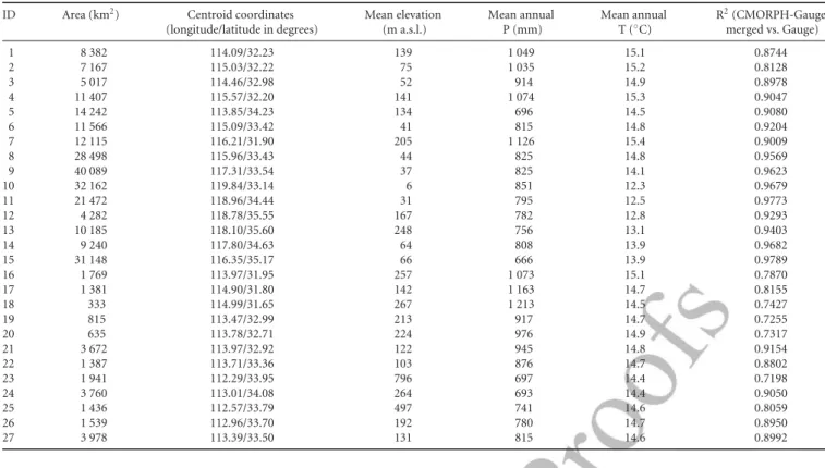
Table 1. Characteristics of the 27 Huai sub-basins.
ID Area (km2) Centroid coordinates Mean elevation Mean annual Mean annual R2(CMORPH-Gauge (longitude/latitude in degrees) (m a.s.l.) P (mm) T (◦C) merged vs. Gauge) 1 8 382 114.09/32.23 139 1 049 15.1 0.8744 2 7 167 115.03/32.22 75 1 035 15.2 0.8128 3 5 017 114.46/32.98 52 914 14.9 0.8978 4 11 407 115.57/32.20 141 1 074 15.3 0.9047 5 14 242 113.85/34.23 134 696 14.5 0.9080 6 11 566 115.09/33.42 41 815 14.8 0.9204 7 12 115 116.21/31.90 205 1 126 15.4 0.9009 8 28 498 115.96/33.43 44 825 14.8 0.9569 9 40 089 117.31/33.54 37 825 14.1 0.9623 10 32 162 119.84/33.14 6 851 12.3 0.9679 11 21 472 118.96/34.44 31 795 12.5 0.9773 12 4 282 118.78/35.55 167 782 12.8 0.9293 13 10 185 118.10/35.60 248 756 13.1 0.9403 14 9 240 117.80/34.63 64 808 13.9 0.9682 15 31 148 116.35/35.17 66 666 13.9 0.9789 16 1 769 113.97/31.95 257 1 073 15.1 0.7870 17 1 381 114.90/31.80 142 1 163 14.7 0.8155 18 333 114.99/31.65 267 1 213 14.5 0.7427 19 815 113.47/32.99 213 917 14.7 0.7255 20 635 113.78/32.71 224 976 14.9 0.7317 21 3 672 113.97/32.92 122 945 14.8 0.9154 22 1 387 113.71/33.36 103 876 14.7 0.8802 23 1 941 112.29/33.95 796 697 14.4 0.7198 24 3 760 113.01/34.08 264 693 14.4 0.9050 25 1 436 112.57/33.79 497 741 14.6 0.8059 26 1 539 112.96/33.70 192 780 14.7 0.8950 27 3 978 113.39/33.50 131 815 14.6 0.8992
Density Function matching algorithm. The corrected CMORPH data are used as the background analysis field; the optimal interpolation algorithm is used in the last step to provide a weighted average precipitation value at each grid point. The final merged dataset results in a spatial 0.1◦×0.1◦grid resolution and hourly time step. The detailed description of the merged dataset can be found in Pan et al.(2012). Shen et al.(2013) assess the quality of this dataset and report it can capture the precipitation process both spatially and temporally very well with low bias and root-mean-square error. The CMORPH-Gauge merged data can be accessed from the CDC’s website. The data are available from 1 January 2008 and near real time with approximately 1 day delay. The time period used in this study is between 0100 UTC 1 January 2008 and 0000 UTC 10 October. At the time of study, this was the longest available time period allowing ten seasons to be analysed.
2.3. ECMWF’s medium-range ensemble forecasts of precipitation
The medium-range ensemble forecasts of precipitation data were obtained from ECMWF. The forecasts of Total Precipitation (TP) were retrieved from ECMWF’s Atmospheric Ensemble Prediction System issued daily at 0000 UTC. It consists of one control forecast, a central analysis driven by a data-assimilation procedure, and 50 perturbed forecasts generated by perturbed initial conditions. The TP data are stored at time steps of T+0 h to T+96 h at 3 h intervals, and then T+96 h to T+240 h at 6 h intervals. The forecast data were interpolated to the same spatial grids as the observational precipitation described in the section above. The 51 forecast members are treated with equal weights. The ensemble forecasts retrieved for this study are from 0000 UTC 1 January 2008 to 0000 UTC 30 September 2012.
3. Experiment design and evaluation scores 3.1. Experiment design
The observed precipitation analysis product, the CMORPH-Gauge merged data, was accumulated to daily time steps and evaluated against the data collected from the basin’s daily rain-gauges which are independent from the hourly gauges used
in the merged dataset. Because the daily rain-gauges record daily precipitation data from Beijing time (UTC+8h) 2100 to Day+1 2100, the CMORPH-Gauge merged data is accumulated from 1300 UTC to Day+1 1300 UTC to be consistent with the rain-gauges. Unlike the hourly rain-gauges used in the CMORPH-Gauge merged data, the data collected from the daily rain-gauge network was quality controlled and contains a larger number of gauges than that of the hourly gauges. The daily rain-gauge data are therefore considered as a reasonable benchmark to cross-check the quality of the CMORPH-Gauge merged data. The correlation between CMORPH-Gauge merged data and daily rain-gauge data was computed for each sub-basin over the entire study time period.
After the quality of the precipitation data was examined, the forecast performance was evaluated. The entire study time period was divided into ten segments, composed of five flooding and five non-flooding seasons. The flooding season covers five months, namely May, June, July, August and September. The non-flooding season covers seven months, namely October, November, December, January, February, March and April. Except for the first segment, the 2008 non-flooding season that covers four months (1 January 2008 to 30 April 2008), the remaining nine segments all span the entire season. The flooding and non-flooding seasons alternate and end with the 2012 flooding season (1 May 2012 to 30 September 2012). The ECMWF ensemble precipitation forecasts were evaluated for all ten seasons, 27 sub-basins, at five different aggregated time steps, namely 3, 6, 12, 24 and 48 h, and all the available lead times.
3.2. Evaluation scores
The Continuous Ranked Probability Score (CRPS:Brown, 1974; Matheson and Winkler, 1976; Hersbach, 2000) and two variants of CRPS were used as evaluation scores. The CRPS is a verification tool that evaluates the degree of agreement between the cumulative probability distribution of an ensemble of variable values with a single observed value.
CRPS=
∞
−∞{P(x)−H(x−xa)}
1 2 3 4 5 6 7 8 9 10 11 12 13 14 15 16 17 18 19 20 21 22 23 24 25 26 27 28 29 30 31 32 33 34 35 36 37 38 39 40 41 42 43 44 45 46 47 48 49 50 51 52 53 54 55 56 57 58 59 60 61 62 63 64 1 2 3 4 5 6 7 8 9 10 11 12 13 14 15 16 17 18 19 20 21 22 23 24 25 26 27 28 29 30 31 32 33 34 35 36 37 38 39 40 41 42 43 44 45 46 47 48 49 50 51 52 53 54 55 56 57 58 59 60 61 62 63 64 wherexis the forecasted variable,xais the actual variable value
(the observed value),P(x) is the cumulative distribution function ofx, andH(x−xa) is the Heaviside function which is 0 when (x−xa)<0 and 1 otherwise. The unit of CRPS is the same as that of x. The ideal degree of agreement (CRPS = 0) is achieved ifP(x)=H(x−xa), which is a perfect deterministic forecast. In practice,CRPSusually takes the average value over an area and a number of forecasting cases. This potentially leads to a technical problem when scores need to be compared amongst different areas, seasons or aggregated time steps when thexvalues can assume various magnitudes. In other words, a lowerCRPSin a particular area or season does not necessarily equate to a better forecasting performance in comparison with another area or season. This is because a lower score can be attributed to lower x values but not a better forecast over a certain area or season. RCRPS, a normalised CRPS, was introduced by Trinhet al.(2013) to handle this technical problem. AQ5
It normalisesCRPSby the standard deviation of the variable of interest.
RCRPS=CRPS σa
, (2)
where σa is the standard deviation of all xa values over a certain area and a number of studied cases. Another normalised form ofCRPSis the Continuous Ranked Probability Skill Score (CRPSS), where CRPS is normalised by a reference which is usually the climatology or persistence of a study area.
CRPSS=1−CRPSF
CRPSR
, (3)
whereCRPSFdenotes the forecast score andCRPSRis the score of a reference forecast of the same variable.CRPSS measures the improvement of an ensemble forecasting system over the reference forecast. Its values range from−∞to 1, where 1 is the ideal forecast and negative values indicate worse performance than the reference forecast. The reference forecast used in this study is climatology, which was computed for flooding or non-flooding seasons respectively over each sub-basin and each accumulated time step using the observed precipitation analysis data from 1
AQ6
January 2008 to 10 October 2012.
The dependency ofCRPSSon sub-basin properties is studied using a multiple regression function. CRPSSis based on 24 h aggregated precipitation and averaged over the five flooding and five non-flooding seasons respectively.
CRPSS=a+b1CS+b2ME+b3MAP, (4) whereais the intercept,biis the coefficient for each variable,CS
is the sub-basin size,MEis the mean elevation, andMAPis the mean annual precipitation. The variablesCS,MEandMAPare all normalised by the maximum of each variable.
4. Results and discussion
4.1. Quality of observed precipitation data
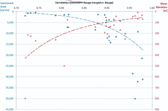
The CMORPH-Gauge merged precipitation dataset is a product based on hourly rain-gauge and satellite data. Its quality was checked against the daily rain-gauge data which is considered as a benchmark. The correlations between the merged data accumulated to 24 hourly (on thex-axis) and the daily rain-gauge data (on they-axis) over the time period between 1 January 2008 and 31 December 2011 were obtained for the 27 sub-basins using linear regression functions (figures are not shown here). The least square errorsR2were computed (last column in Table 1). The correlations are generally better for larger sub-basins and sub-basins with lower elevations (Figure 2), and vice versa. The
y-intercepts obtained for all the 27 linear regression functions are positive, indicating underestimation of precipitation in the CMORPH-Gauge merged data in comparison with the daily rain-gauge data. Xie et al.(2007) reports a similar finding that the CMORPH product underestimates the precipitation amount over eastern China. The sub-basins with the largest and smallest
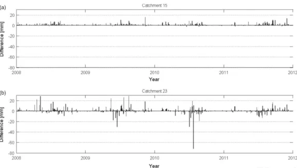
R2 are sub-basin no. 15 with an area of 31 148 km2 and mean elevation of 66 m, and sub-basin no. 23 with an area of 1941 km2 and mean elevation of 796 m (Figure 3).
The advantage of using the merged data lies in its high spatial and temporal resolutions which make it possible to evaluate forecast performance at sub-daily time-scales. The correlations for the 27 sub-basins are all above 0.7 and acceptable. Nevertheless, the uncertainties associated with the skill scores caused by the limitation in the high spatial and temporal resolution precipitation analysis product need to be recognised.
Color Figure -Online o nly
Figure 2.The relationship between sub-basin areas (left axis, diamond markers)/mean elevation (right axis, triangular markers) and correlations R2(between
CMORPH-Gauge merged and rain-gauge precipitation time series at 24 h intervals). Correlations are higher for larger sub-basins and sub-basins dominated by flat terrains (refer to the last column in Table 1 for the correlation R2). This figure is available in colour online at wileyonlinelibrary.com/journal/qj
1 2 3 4 5 6 7 8 9 10 11 12 13 14 15 16 17 18 19 20 21 22 23 24 25 26 27 28 29 30 31 32 33 34 35 36 37 38 39 40 41 42 43 44 45 46 47 48 49 50 51 52 53 54 55 56 57 58 59 60 61 62 63 64 1 2 3 4 5 6 7 8 9 10 11 12 13 14 15 16 17 18 19 20 21 22 23 24 25 26 27 28 29 30 31 32 33 34 35 36 37 38 39 40 41 42 43 44 45 46 47 48 49 50 51 52 53 54 55 56 57 58 59 60 61 62 63 64 (a) (b)
Figure 3.(a), (b) The difference in the daily precipitation time series (rain gauge – CMORPH-Gauge merged) for the best and worst correlated sub-basins nos. 15 and 23 respectively. In the majority of cases the CMORPH-Gauge merged data underestimate the daily precipitation values. The precipitation data in 2012 were not evaluated because the quality control of the daily rain-gauge data would not be completed until the first quarter of 2013.
4.2. The overall skill scores of ECMWF’s ensemble forecasts CRPSSis used to evaluate the overall performance of ECMWF’s ensemble forecasts in comparison with climatology. Figure 4 showsCRPSScalculated using 24 h accumulated precipitation and averaged over the five flooding and five non-flooding seasons respectively. Sub-plots are presented in ascending order of sub-basin size. All sub-basins, except nos. 5, 12, 13, 23, 24 and 25, in both flooding and non-flooding seasons show overall decreasing skill scores with increasing lead times for the forecasted precipitation. The six atypical sub-basins exhibit rising or fluctuating skill scores with increasing lead times. Sub-basins nos. 5, 23, 24 and 25 are located towards the north-west of the basin dominated by the Tongbai mountains, and sub-basins nos. 12 and 13 are located towards the north-east dominated by the Yimeng mountain ranges. The ensemble forecasts completely failed to show any skill in these six sub-basins all located between 34◦N and 36◦N and characterised by high altitudes. This may suggest the need for local models in the areas dominated by high altitude to resolve rain-driven processes at small scales.
The skill scores vary depending on the seasons and the sizes of the sub-basins. Flooding seasons (line with dots) showed higher skill scores than non-flooding seasons (line with circles). This may indicate it is easier to correctly forecast rain occurrence and magnitude in a wet season than in a dry season, and the forecasts tend to be more skilful in the wet season compared to the dry season. CRPSS for the flooding seasons never drops below 0, which means the forecasted precipitation for all 27 sub-basins was more skilful than their climatology. For sub-basins smaller than 2000 km2(the first row of sub-basins in Figure 4) except nos. 23 and 25, the highest scores never exceeded 0.4 during flooding seasons. The scores are much lower during the non-flooding seasons and most of them show no skill at all (CRPSS<0). For the sub-basins smaller than 10 000 km2(the second row of sub-basins in Figure 4) except nos. 12, 13 and 24, the scores appear to be better than the first row of sub-basins. The best scores were achieved by the sub-basins larger than 10 000 km2(the last row of sub-basins in Figure 4) except no. 5. In general, the forecast skill improves as the sub-basin size increases, and forecasts in the flooding seasons outperform those in the non-flooding seasons.
For midlatitude sub-basins like the ones in the Huai river basin, ECMWF’s ensemble forecasts can be used in forecasting floods with relatively low, medium and high confidence during flooding seasons for sub-basins with sizes<2000, 2000–10 000, >10 000 km2 respectively. The exception here is the sub-basin
dominated by high elevations. During non-flooding seasons, ECMWF’s ensemble forecasts did not show satisfactory skills for sub-basins smaller than 2000 km2, but some reasonable skill for sub-basins larger than 2000 km2. Overall, the forecasts are more skilful in the flooding seasons than the non-flooding seasons over this midlatitude river basin.
4.3. Skill dependency on sub-basin properties and seasons
The dependency of CRPSS on sub-basin properties is further studied using the multiple regression function (Eq. (4) in section 3.2).CRPSSis based on 24 h accumulated precipitation and averaged over the five flooding and five non-flooding seasons respectively, the same as what was used in Figure 4.
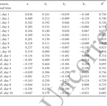
Sub-basins nos. 5, 12, 13, 23, 24 and 25 were excluded from finding the multiple regression function due to their unusual pattern ofCRPSSalready discussed in section 4.2. In addition, sub-basins nos. 4 and 7 were also excluded because they do not exhibit homogeneous sub-basin properties with respect to elevation and may interfere with the results. The two sub-basins in question have a large portion of high elevation towards the south side but are fairly flat towards the north. After excluding the seven sub-basins, the obtained regression function based on the remaining 20 sub-basins for the flooding season is given in Table 2.
For the flooding seasons, the coefficients of determinationR2of all ten lead times are no less than 0.655 (lowest value appeared on day 5), which indicates that the obtained regression can account for at least 65.5% of the original variability and the regression model fit is satisfactory. Figure 5 shows an example of the fitted
CRPSSversus the original CRPSS for the flooding season on day 2. For flooding seasons, the coefficients ofCS(b1) for the ten lead times are all positive, implying CRPSSincreases with increase ofCS. The coefficients ofME(b3) are mostly negative (except days 3–5) and close to 0. This meansMEhas a relatively smaller influence on CRPSS than CS and MAP have during flooding seasons. In most cases the higher the mean elevation of a sub-basin is, the lower is theCRPSS. The absolute values of the coefficients ofMAP(b3) exhibit an interesting decreasing trend up to day 4 and then an increasing trend from days 6 to 10. Except day 5 which shows a positive relation betweenCRPSSand
MAP, all other nine days have negative values, suggesting that wetter sub-basins with higher mean annual precipitation tend to have lowerCRPSSand the ensemble forecasts are less capable for wetter sub-basins. The degree of negative relationship between
1 2 3 4 5 6 7 8 9 10 11 12 13 14 15 16 17 18 19 20 21 22 23 24 25 26 27 28 29 30 31 32 33 34 35 36 37 38 39 40 41 42 43 44 45 46 47 48 49 50 51 52 53 54 55 56 57 58 59 60 61 62 63 64 1 2 3 4 5 6 7 8 9 10 11 12 13 14 15 16 17 18 19 20 21 22 23 24 25 26 27 28 29 30 31 32 33 34 35 36 37 38 39 40 41 42 43 44 45 46 47 48 49 50 51 52 53 54 55 56 57 58 59 60 61 62 63 64 Figure 4.The meanCRPSSversus lead times for each sub-basin in flooding seasons (line with dots) and non-flooding seasons (line with circles). The score is calculated using 24 h accumulated precipitation. Sub-plots are presented in ascending order of the sub-basin size. The numbers above each sub-plot are the sub-basin no., size, mean elevation, and mean annual precipitation respectively.
Table 2. The intercepts, coefficients and coefficients of determinationR2of the
multiple regression ofCRPSSfor flooding and non-flooding seasons at different lead times. Season, a b1 b2 b3 R2 lead time F, day 1 0.636 0.161 −0.034 −0.348 0.756 AQ7 F, day 2 0.400 0.212 −0.009 −0.159 0.740 F, day 3 0.342 0.192 0.046 −0.154 0.720 F, day 4 0.285 0.152 0.012 −0.066 0.719 F, day 5 0.164 0.140 0.020 0.067 0.655 F, day 6 0.209 0.124 −0.002 −0.011 0.682 F, day 7 0.201 0.130 −0.046 −0.013 0.819 F, day 8 0.218 0.111 −0.034 −0.088 0.818 F, day 9 0.237 0.102 −0.007 −0.150 0.823 F, day 10 0.319 0.090 −0.002 −0.278 0.834 nF, day 1 −0.116 0.354 −0.481 0.488 0.714 nF, day 2 −0.301 0.489 −0.450 0.514 0.684 nF, day 3 −0.159 0.464 −0.366 0.184 0.693 nF, day 4 −0.197 0.430 −0.363 0.190 0.741 nF, day 5 −0.020 0.306 −0.299 −0.026 0.756 nF, day 6 −0.081 0.273 −0.358 0.053 0.763 nF, day 7 −0.163 0.250 −0.273 0.124 0.729 nF, day 8 −0.044 0.214 −0.233 0.008 0.735 nF, day 9 −0.256 0.238 −0.180 0.175 0.687 nF, day 10 −0.047 0.179 −0.141 −0.051 0.685
CRPSSandMAPdecreases from days 1 to 4 then increases from days 6 to 10. It may indicate that wetness influence onCRPSS
initially dominates on day 1, and continues to decline from day 2. The wetness influence is taken over by the sub-basin sizeCS
up until day 4, after which its influence onCRPSSrises again to eventually take overCS.
For the non-flooding seasons, the coefficients of determination
R2of all ten lead times are generally lower than the ones obtained for the flooding seasons. The coefficient b1 is positive for all ten lead times, indicating the forecast skill improves as the sub-basin size increases. The coefficientb2is always negative and the absolute values are comparably larger than those in the flooding seasons. This means the forecast skill may be affected more by
Figure 5.The original and the fitted CRPSS using the multiple regression function (flooding season, day 2).
the sub-basin mean elevation when orographic rain events may occur more during the non-flooding seasons. The coefficientb3 is mostly positive except on days 5 and 10. It does not show any increasing or decreasing trend as what can be seen in the flooding seasons. The forecast skill tends to be better for those sub-basins with higher mean annual precipitation. It may be easier to forecast rain occurrence and magnitude in a relatively wetter non-flooding season than a drier one.
4.4. Skill dependency on lead times and aggregation of time steps
The three evaluation scores CRPS, RCRPS and CRPSS were computed at an aggregation of five time steps, namely 3, 6, 12, 24 and 48 h, and all available lead times to investigate whether or not the forecast skill depends on the aggregation of time steps and lead times. The obtained scores were then averaged for the five
1 2 3 4 5 6 7 8 9 10 11 12 13 14 15 16 17 18 19 20 21 22 23 24 25 26 27 28 29 30 31 32 33 34 35 36 37 38 39 40 41 42 43 44 45 46 47 48 49 50 51 52 53 54 55 56 57 58 59 60 61 62 63 64 1 2 3 4 5 6 7 8 9 10 11 12 13 14 15 16 17 18 19 20 21 22 23 24 25 26 27 28 29 30 31 32 33 34 35 36 37 38 39 40 41 42 43 44 45 46 47 48 49 50 51 52 53 54 55 56 57 58 59 60 61 62 63 64 flooding and non-flooding seasons respectively. Figure 6 shows
the three evaluation scores averaged for (a) the five flooding seasons and (b) the five non-flooding seasons for three selected sub-basins. They are no. 16 (blue dotted lines), 14 (black lines marked with circles) and 10 (red lines marked with crosses). They AQ8
are randomly selected from each of the three rows of sub-basins shown in Figure 4 to represent three categories of sub-basin sizes. The left, middle and right panels in Figure 6 areCRPS,
RCRPSandCRPSSrespectively. The rows from top to bottom correspond to five aggregated time steps from 3, 6, 12, 24 to 48 h respectively. Because the ECMWF archives forecasts from T+0 h to T+96 h at 3 h intervals, the first row of scores ends at T+96 h.
Across the five aggregated time steps, one can see the forecast performance generally deteriorate as the lead times increase, but fluctuate up and down for the 3, 6 and 12 h time steps. The fluctuating pattern is prominent and seems to follow a periodic cycle every day with an inflexion point occurring after half a day, hence referred to as the diurnal cycle. This particular diurnal cycle will be further discussed in section 4.5.
It can be observed from theCRPSin Figure 6 that the forecast performance seems to worsen significantly as the time step increases from 3 to 48 h (values increase from around 0.5 to 5). Because the forecasted variable, precipitation in this study, can assume different magnitudes when it represents different areas, seasons or aggregated time steps, CRPS becomes an
(a)
(b)
Figure 6.Three performance scores averaged for (a) the five flooding seasons and (b) the five non-flooding seasons for sub-basins nos. 16 (dashed line with dots), 14 (line with circles) and 10 (line with asterisks). Left, middle and right panels areCRPS,RCRPSandCRPSSrespectively. The rows from top to bottom correspond to the aggregated time steps of 3, 6, 12, 24 and 48 h respectively. Because ECMWF archives ensemble forecasts from T+0 h to T+96 h at 3 h intervals, the first row of scores end at T+96 h.
1 2 3 4 5 6 7 8 9 10 11 12 13 14 15 16 17 18 19 20 21 22 23 24 25 26 27 28 29 30 31 32 33 34 35 36 37 38 39 40 41 42 43 44 45 46 47 48 49 50 51 52 53 54 55 56 57 58 59 60 61 62 63 64 1 2 3 4 5 6 7 8 9 10 11 12 13 14 15 16 17 18 19 20 21 22 23 24 25 26 27 28 29 30 31 32 33 34 35 36 37 38 39 40 41 42 43 44 45 46 47 48 49 50 51 52 53 54 55 56 57 58 59 60 61 62 63 64 incomparable evaluation score. One needs to use RCRPS or
CRPSS if performance comparison needs to be made across different areas, seasons or aggregated time steps. RCPRS is simply a normalised score disregarding the magnitude of the forecasted variable.CRPSSdoes not only eliminate the effect of the magnitude of the forecasted variable, it also compares the forecasts with the relevant climatology. Therefore,RCRPS and
CRPSSare considered in the following comparison. BothRCRPS
andCRPSSdemonstrate fluctuating patterns for the sub-daily time steps. The scores show evident improvement from 3, 6, 12 to 24 h time step. The improvement from 24 to 48 h is only marginal. This suggests that the forecast performance improves as the aggregation of time steps becomes larger, although marginal once aggregation exceeds 24 h. Sub-basin no. 10 shows the best performance with respect toCRPSS, followed by no. 14, and the worst is no. 16. This reflects the relationship betweenCRPSSand sub-basin size which has already been discussed in section 4.3. In comparison, Figure 6(b) shows the average scores for the non-flooding seasons. Similar fluctuating patterns can be observed for the sub-daily time steps, but their phases are different from sub-basin to sub-basin.
4.5. Sub-daily skill
To study the diurnal cycle in detail, the meanCRPSvalue of the five flooding and five non-flooding seasons for each of the 27 sub-basins at five different aggregated time steps was computed and is shown in Figure 7. ECMWF archives precipitation forecasts at time steps of T+0 h to T+96 h at 3 h intervals. This is the reason why Figure 7(a) ends at 96 h whereas the other four time steps all run up to 240 h. During the flooding seasons,CRPSvalues in Figure 7(a) of all 27 sub-basins generally increase with the increase of lead times and at a fairly constant pace. In other words, the forecast performance worsens constantly over the lead times, but with the exception of the scores computed at sub-daily time steps. For the 3 h time step, theCRPSvalues of most sub-basins decrease from 0300 UTC to a daily minimum at around 1500 UTC (±3 h depending on the sub-basin). They then rise to a daily maximum at around Day+1 0300 UTC (some sub-basins show a small drop between 2100 UTC and 2400 UTC). In other words, the first daily cyclic change inCRPSis a decline from 0300 UTC to 1500 UTC (±3 h) that lasts approximately 12 h, and the second change is a growth from 1500 UTC (±3 h) to Day+1 0300 UTC that lasts for another 12 h. These time intervals correspond to the Beijing time 1100–2300 for the decline and 2300–Day+1 1100 for the growth. The daily minimumCRPShappens at around Beijing time 2300. In terms of the forecast performance, it improves from Beijing time 1100 to 2300 and then drops in the next 12 h. For the non-flooding seasons, the diurnal pattern is not as obvious as for the flooding season. TheCRPSvalues for the 3 h time interval during the non-flooding seasons seem to fluctuate randomly with a very gentle increasing trend. In Figure 7(b), the diurnal pattern with the same decline and growth cycles as those of the 3 h can be clearly seen for the flooding season. For the non-flooding season, the pattern is weak and not consistent for all the sub-basins. In Figure 7(c), the meanCRPSvalues computed at 12 h time steps show a different diurnal pattern from those of the 3 and 6 h time steps. The daily decline starts from 1200 UTC and ends at 2400 UTC, which is followed by a growth from 2400 to 1200 UTC. While the majority of sub-basins show this pattern, there are a number of sub-basins that exhibit a rather opposite pattern. This could be due to the fact that the forecasted precipitation is aggregated for every 12 h (i.e. 0000–1200, 1200–2400 UTC, etc.) and the aggregation has interfered with the actual dynamics of the rainfall events. Additionally, diurnal cycles vary with the locations of the sub-basins. In Figure 7(d), the forecast performance for both flooding and non-flooding seasons deteriorates rapidly till Day 3 (72 h) which is shown as an increase in the meanCRPS
values for all the 27 sub-basins. From the 72th to the 240th hour, the rate of increase slows down slightly, especially after the
144th hour (Day 6). In Figure 7(e), the turning point of the mean
CRPSvalues occurs at the 96th hour. Because the precipitation values are aggregated for every 48 h, it is impossible to capture the same turning point as in Figure 7(d).
The diurnal cycle in the observed precipitation for May–September in the domain of central-east China (105–120◦E, 26–36◦N) was reported in Yuet al.(2007a, 2007b). The Huai river basin is located in the upper east of this domain. Their results show that the rainfall events of duration between 1 and 3 h peak around late afternoon, which may be explained by the diurnal variation of surface solar heating that influences the diurnal variation of low-level atmospheric stability. Rainfall events of duration longer than 6 h dominate (>60% of the total precipitation) in this domain and they tend to peak in the early morning of each day. The reason for this peak is more complex than for the late afternoon one. Nesbitt and Zipser (2003) sug-gest the nocturnal rain is often caused by mesoscale convective systems (MCS) rather than isolated convection, and the MCS is the strongest after midnight. Chenet al.(1998, 2000) and Sun
et al.(2005) point out that heavy rainfall of the summer Meiyu
front mostly results from well organised MCS overlapping the distinctive stratus cloud. The diurnal pattern of the forecast-ing performance observed in the floodforecast-ing season may suggest ECMWF’s EPS is weak in capturing the MCS and hence the early morning peaks. There are limited numbers of studies that verify diurnal cycles of NWP-modelled precipitation, although the ability of NWP to capture diurnal precipitation cycles cannot be understated. The diurnal cycles in the mesoscale NWP model from MeteoSwiss are verified using hourly rain-gauge data by Kaufmann et al.(2003). They find the model performs well in winter because there is no diurnal forcing, but fails to reproduce diurnal cycles in summer. The convection starts too early and lasts a very short time in this model and overestimates the amount of precipitation. Guichard et al.(2004) investigate modelling of the diurnal cycle of deep precipitating convection over land using seven single-column models (SCMs) and three cloud-resolving models (CRMs). It was found convection occurs too early in most SCMs due to crude triggering criteria. In the CRMs, the first clouds appear before noon, but surface rainfall is delayed by several hours.
The intra-daily precipitation dynamics were looked at by aggregating both the forecasted and observed precipitation to the multiple of 3 h from 3 up to 24 h. Figure 8 shows (a) the observed and (b) forecasted mean of the daily aggregated precipitation within each season and for all the 27 sub-basins. In the case of the forecasted mean of the daily aggregated precipitation, it was computed as the mean of the 51 ensemble members for the first eight time steps (Day 1) only. The dark black line is the mean of the mean of the 27 daily aggregated precipitation series. During the non-flooding seasons, there are two major differences between the observed and the forecasted: (i) the spread of the blue lines for the 27 sub-basins is larger in the observed than in the forecasted precipitation; and (ii) the aggregated precipitation values obtained from ensemble forecasts are larger than those from the observed. During the flooding seasons, in addition to the smaller spread in the forecasted daily precipitation, the major contrast lies in the intra-daily precipitation dynamics. The black lines obtained from the observed precipitation are fairly linear, whereas the black lines obtained from the forecasted precipitation show an obvious turning point at the ninth hour in a day. The turning point cannot directly explain the diurnal pattern in the
CRPSvalues obtained for the flooding seasons, but it does indicate that the intra-daily rainfall dynamics are not well simulated by ECMWF’s EPS.
5. Conclusion and outlook
This study has evaluated the performance of ECMWF’s medium-range ensemble forecasts of precipitation for the Huai river basin, a midlatitude basin covering a considerably large area
1 2 3 4 5 6 7 8 9 10 11 12 13 14 15 16 17 18 19 20 21 22 23 24 25 26 27 28 29 30 31 32 33 34 35 36 37 38 39 40 41 42 43 44 45 46 47 48 49 50 51 52 53 54 55 56 57 58 59 60 61 62 63 64 1 2 3 4 5 6 7 8 9 10 11 12 13 14 15 16 17 18 19 20 21 22 23 24 25 26 27 28 29 30 31 32 33 34 35 36 37 38 39 40 41 42 43 44 45 46 47 48 49 50 51 52 53 54 55 56 57 58 59 60 61 62 63 64 (a) (b) (c) Color Figure -O nline o nly
Figure 7.The meanCRPSover five flooding (left panels) and five non-flooding (right panels) seasons for the 27 sub-basins computed at five aggregated time steps:
AQ9
1 2 3 4 5 6 7 8 9 10 11 12 13 14 15 16 17 18 19 20 21 22 23 24 25 26 27 28 29 30 31 32 33 34 35 36 37 38 39 40 41 42 43 44 45 46 47 48 49 50 51 52 53 54 55 56 57 58 59 60 61 62 63 64 1 2 3 4 5 6 7 8 9 10 11 12 13 14 15 16 17 18 19 20 21 22 23 24 25 26 27 28 29 30 31 32 33 34 35 36 37 38 39 40 41 42 43 44 45 46 47 48 49 50 51 52 53 54 55 56 57 58 59 60 61 62 63 64 (d) (e) Color Figure -O nline o nly
Figure 7.Continued This figure is available in colour online at wileyonlinelibrary.com/journal/qj
(270 000 km2) representing various geographic and climatic properties. Precipitation forecasts were evaluated in a way relevant to the hydrological processes of runoff, by considering the river basin (and sub-basin) as the spatial units of evaluation as opposed to large aggregated grid-based areas. Only in this way can it be said whether the forecasts have the potential to be useful for hydrological prediction such as flood forecasting. It is strongly recommended that this becomes the norm for precipitation forecast evaluation.
For the observed precipitation, it was found that the CMORPH-Gauge merged dataset proves to be of good quality when cross-checked with the daily rain-gauge data. The dataset enabled detailed forecast performance evaluation at sub-daily scales for the first time. The dataset covers almost 5 years which allowed a long-term and continuous evaluation, rather than event-based studies. Such continuous evaluation is essential for truly understanding the quality of any forecasting system. The CMORPH-Gauge merged dataset systematically underestimates precipitation, especially high precipitation and this bias should be corrected for different months, seasons and areas to give a more credible evaluation of the forecast performance. This dataset is especially valuable in the assessment of EPS at sub-daily scales, as the sub-sub-daily precipitation can be important in hydrological applications (e.g. Wetterhall et al., 2011; Parkeset al., 2013).
Precipitation forecast performance was found to vary with sub-basin properties, aggregated time steps and lead times, and between flooding and non-flooding seasons. This highlights two salient points: forecast performance can only be evaluated effectively if the forecast parameters are understood (lead time, time step) but also importantly if the hydrogeographical attributes of the study area are also considered (e.g. basin elevation, flood seasonality, etc.). The study provides answers to the three scientific questions proposed in the introduction:
(i) For midlatitude sub-basins like the ones in the Huai river basin, ECMWF’s ensemble forecasts can be used in forecasting floods with relatively low, medium and high confidence during flooding seasons for sub-basins with sizes<2000, 2000–10 000 and>10 000 km2respectively. The exception is the sub-basin dominated by high elevations. During non-flooding seasons, no satisfactory skills were found for the sub-basins smaller than 2000 km2 but some reasonable skills for the sub-basins larger than 2000 km2. Overall, the forecasts are more skilful in the flooding seasons than the non-flooding seasons over this basin.
(ii) The forecast skill at each sub-basin depends on the three studied sub-basin hydrogeographical properties of basin size, mean annual precipitation and mean elevation, to various extents, and seasons as well. Because the obtained
1 2 3 4 5 6 7 8 9 10 11 12 13 14 15 16 17 18 19 20 21 22 23 24 25 26 27 28 29 30 31 32 33 34 35 36 37 38 39 40 41 42 43 44 45 46 47 48 49 50 51 52 53 54 55 56 57 58 59 60 61 62 63 64 1 2 3 4 5 6 7 8 9 10 11 12 13 14 15 16 17 18 19 20 21 22 23 24 25 26 27 28 29 30 31 32 33 34 35 36 37 38 39 40 41 42 43 44 45 46 47 48 49 50 51 52 53 54 55 56 57 58 59 60 61 62 63 64 (a) (b) Color Figure -Online o nly
Figure 8.The (a) observed and (b) forecasted mean of the aggregated precipitation within each season and for all the 27 sub-basins. x-axis is the aggregated time in
AQ10
hours. y-axis is the precipitation in mm. The ‘nf’ and ‘f’ above each sub-plot stands for ‘non-flooding season’ and ‘flooding season’ respectively. The dashed line is the mean (the 27 sub-basins) of the mean (51 ensemble members) of the daily aggregated precipitation of the 27 sub-basins. This figure is available in colour online at wileyonlinelibrary.com/journal/qj
regression model does not account for the total variability in CRPSS, other variables that can affect the forecast performance may need to be considered. Regardless of the season, larger sub-basins benefit from better forecast skills because the current forecast model is still limited in resolving small-scale events. One needs to be cautious when applying these ensemble forecasts in small-scale sub-basins, especially those smaller than 2000 km2. The higher the sub-basin’s mean annual precipitation, the lower theCRPSS. This means the ensemble forecasts are less capable for wetter sub-basins, and in particular for the extreme events. The comparatively lower CRPSSduring non-flooding seasons indicate the ensemble forecasts are less skilful in simulating rain occurrence and magnitude in dry seasons. The drier the sub-basin, the more challenges it presents to the model to correctly forecast the rain.
ECMWF’s EPS does a fairly satisfactory job in forecasting medium-range precipitation, but needs to improve in forecasting very high or low precipitation. The forecast skill also depends on lead times and aggregation of time steps. Forecast performance worsens as the lead time increases. The forecast performance improves as the time steps are aggregated from 3, 6, 12 to 24 h time step. The improvement from 24 to 48 h is marginal.
(iii) In flooding seasons, the evaluation scores at sub-daily steps present a prominent and consistent diurnal cycle for all the 27 sub-basins. The forecast performance improves from Beijing time 1100 to 2300 and then drops in the next 12 h. In non-flooding seasons, the diurnal cycle also exists at sub-daily time steps, although not consistently across the 27 sub-basins. The reasons for the diurnal cycle in observed precipitation are still not well understood.
1 2 3 4 5 6 7 8 9 10 11 12 13 14 15 16 17 18 19 20 21 22 23 24 25 26 27 28 29 30 31 32 33 34 35 36 37 38 39 40 41 42 43 44 45 46 47 48 49 50 51 52 53 54 55 56 57 58 59 60 61 62 63 64 1 2 3 4 5 6 7 8 9 10 11 12 13 14 15 16 17 18 19 20 21 22 23 24 25 26 27 28 29 30 31 32 33 34 35 36 37 38 39 40 41 42 43 44 45 46 47 48 49 50 51 52 53 54 55 56 57 58 59 60 61 62 63 64 The result suggests ECMWF’s ensemble forecasts may be
unsuccessful in capturing the nocturnal cycle and the MCS in the study domain. The result also shows the intra-daily rainfall dynamics are not well simulated by ECMWF’s EPS and hence the sub-daily ensemble forecasts generated by the current model version do not benefit the forecasters. The model performance at sub-daily steps and reasons for failures need to be studied in more detail in the future. The Huai river basin used in this study was selected because it is representative of many types of river basins around the world and thus conclusions can be to some extent generalised. It can be said that ECMWF EPS precipitation forecasts are generally skilful for flood forecasting especially in large river sub-basins. However, future research is encouraged in other areas of the world and even at the global scale (Alfieriet al., 2013). Future research could also consider in more detail the impact of post-processing methods (Schaakeet al., 2010) and the nature of the rainfall patterns and intensities during flood seasons. As the use of EPS forecasts in flood forecasting becomes more widespread across the globe, studies of this nature will become increasingly important in providing benchmarks for operational forecasting. Evaluating precipitation forecasts in a hydrologically relevant way, as demonstrated in this study, is essential in order to fully understand forecast performance.
6. Acknowledgements
This study was partially financed by the UK ESRC research project ‘Improving the communication and use of ensemble flood predictions’ (RES-189-25-0286) and partially supported by the National Natural Science Foundation of China (41130639 and 51179045) and China Meteorological Administration Special Public Welfare Research Fund (GYHY201006037). The observed precipitation data were provided by the Climatic Data Centre, National Meteorological Information Centre, China Meteorological Administration. We thank the two anonymous reviewers for their careful revision, which helped improve this manuscript.
References
Alfieri L, Salamon P, Pappenberger F, Wetterhall F, Thielen J. 2012. Operational early warning systems for water-related hazards in Europe.Environ. Sci. Policy 21: 35–49, DOI: 10.1016/j.envsci.2012.01.008.
Alfieri L, Burek P, Dutra E, Krzeminski B, Muraro D, Thielen J, Pappenberger F. 2013. GloFAS – Global ensemble streamflow forecasting and flood early warning. Hydrol. Earth Syst. Sci.17: 1161–1175, DOI: 10.5194/hess-17-1161-2013.
Bao C-L. 1987.Synoptic Meteorology in China.Springer-Verlag: Berlin. Bougeault P, Toth Z, Bishop C, Brown B, Burridge D, Chen D, Ebert E,
Fuentes M, Hamill T, Mylne KR, Nicolau J, Paccagnella T, Park Y-Y, Parsons D, Raoult B, Schuster D, Silva Dias P, Swinbank R, Takeuchi Y, Tennant W, Wilson L, Worley S. 2010. The THORPEX Interactive Grand Global Ensemble (TIGGE).Bull. Am. Meteorol. Soc.91: 1059–1072. Br¨ocker J. 2012. Evaluating raw ensembles with the continuous ranked
probability score.Q. J. R. Meteorol. Soc.138: 1611–1617, DOI: 10.1002/ qj.1891.
Brown TA. 1974.Admissible Scoring Systems for Continuous Distributions,
Manuscript P-5235.The Rand Corporation: Santa Monica, CA. Available
from The Rand Corporation, 1700 Main St., Santa Monica, CA 90407-2138. Buizza R. 2008. The value of probabilistic prediction.Atmos. Sci. Lett.9: 36–42,
DOI: 10.1002/asl.170.
Chen S-J, Kuo Y-H, Wang W, Tao Z-Y, Cui B. 1998. A modeling case study of heavy rainstorms along the Meiyu front.Mon. Weather Rev.126: 2330–2351, DOI: 10.1175/1520-0493(1998)126<2330:AMCSOH>2.0.CO;2.
Chen S-J, Wang W, Lau K-H, Zhang Q-H, Chung Y-S. 2000. Mesoscale convective systems along the Meiyu front in a numerical model.Meteorol.
Atmos. Phys.75: 149–160.
Cheng H-Q. 2004. ‘Spatial variation, causes and forecasting models of storm
AQ11
events in the Huai River basin’, Masters thesis, Chinese Academy of
AQ12 Meteorological Sciences. Unpublished (in Chinese).
Cloke HL, Pappenberger F. 2008. Evaluating forecasts of extreme events for hydrological applications: An approach for screening unfamiliar performance measures.Meteorol. Appl.15: 181–197.
Cloke HL, Pappenberger F. 2009. Ensemble flood forecasting: A review.
J. Hydrol.375: 613–626.
Demeritt D, Nobert S, Cloke HL, Pappenberger F. 2010. Challenges in communicating and using ensembles in operational flood forecasting.
Meteorol. Appl.17: 209–222, DOI: 10.1002/met.194.
De Roo A, Thielen J, Salamon P, Bogner K, Nobert S, Cloke HL, Demeritt D, Younis J, Kalas M, Bodis K, Muraro D, Pappenberger F. 2011. Quality control, validation and user feedback of the European Flood Alert System (EFAS).Int. J. Digital Earth4:(Suppl. 1): 77–90.
Fu A. 1991.A Brief Introduction of River System in Hongruhe River Basin.
Henan Province Prospecting and Designing Institute of Water Conservancy:
Zhengzhou. Unpublished. AQ13 Guichard F, Petch JC, Redelsperger J-L, Bechtold P, Chaboureau J-P, Cheinet S,
Grabowski W, Grenier H, Jones CG, K¨ohler M, Piriou J-M, Tailleux R, Tomasini M. 2004. Modelling the diurnal cycle of deep precipitating convection over land with cloud-resolving models and single-column models.Q. J. R. Meteorol. Soc.130: 3139–3172, DOI: 10.1256/qj.03.145. Hamill TM, Mullen SL, Snyder C, Baumhefner DP, Toth Z. 2000.
Ensemble forecasting in the short to medium range: Report from a workshop.Bull. Am. Meteorol. Soc.81: 2653–2664, DOI: 10.1175/1520-0477 (2000)081<2653:EFITST>2.3.CO;2.
He Y, Wetterhall F, Cloke HL, Pappenberger F, Wilson M, Freer J, McGregor G. 2009. Tracking the uncertainty in flood alerts driven by grand ensemble weather predictions.Meteorol. Appl.16: 91–101, DOI: 10.1002/met.132. He Y, Wetterhall F, Bao H-J Cloke HL, Li Z-J, Pappenberger F, Hu Y-Z,
Manful D, Huang Y-C. 2010. Ensemble forecasting using TIGGE for the July–September 2008 floods in the Upper Huai sub-basin – A case study.
Atmos. Sci. Lett.11: 132–138, DOI: 10.1002/asl.270.
Hersbach H. 2000. Decomposition of the continuous ranked probability score for ensemble prediction systems.Weather and Forecasting15: 559–570, DOI: 10.1175/1520-0434(2000)015<0559:DOTCRP>2.0.CO;2.
Huai River Commission, Ministry of Water Resources. 1999.Atlas of Huai
River Basin.Science Press: Beijing.
Huai River Commission, Ministry of Water Resources. 2010.Huai River Storms
and Floods in 2007.China Water Power Press: Beijing (in Chinese).
Joyce RJ, Janowiak JE, Arkin PA, Xie P. 2004. CMORPH: A method that produces global precipitation estimates from passive microwave and infrared data at high spatial and temporal resolution.J. Hydrometeorol.5: 487–503. Kaufmann P, Schubiger F, Binder P. 2003. Precipitation forecasting by a
mesoscale numerical weather prediction (NWP) model: Eight years of experience.Hydrol. Earth Syst. Sci.7: 812–832, DOI: 10.5194/hess-7-812-2003.
Leith CE. 1974. Theoretical skill of Monte Carlo forecasts.Mon. Weather. Rev.102: 409–418, DOI: 10.1175/1520-0493(1974)102<0409:TSOMCF>
2.0.CO;2.
Liu Y, Duan Q, Zhao L, Ye A, Tao Y, Miao C, Mu X, Schaake JC. 2013. Evaluating the predictive skill of post-processed NCEP GFS ensemble precipitation forecasts in China’s Huai river basin. Hydrol. Process. 27: 57–74, DOI: 10.1002/hyp.9496.
Lorenz EN. 1963. Deterministic nonperiodic flow.J. Atmos. Sci.20: 130–141. Lorenz EN. 1969. The predictability of a flow which possesses many scales of
motion.Tellus21: 289–307.
Matheson JE, Winkler RL. 1976. Scoring rules for continuous probability distributions.Manage. Sci.22: 1087–1095.
Molteni F, Buizza R, Palmer TN, Petroliagis T. 1996. The ECMWF Ensemble Prediction System: Methodology and validation.Q. J. R. Meteorol. Soc.122: 73–119, DOI: 10.1002/qj.49712252905.
Nesbitt SW, Zipser EJ. 2003. The diurnal cycle of rainfall and convective intensity according to three years of TRMM measurements.J. Climate16: 1456–1475.
Ning Y, Qian M, Wang Y-T. 2003.Huai River Basin Hydraulic Handbook.
Science Press: Beijing (in Chinese).
Pan Y, Shen Y, Yu JJ, Zhao P. 2012. Analysis of the combined gauge–satellite hourly precipitation over China based on the OI technique.Acta Meteorol. Sin.70: 1381–1389 (in Chinese with an English abstract).
Pappenberger F, Buizza R. 2009. The skill of ECMWF predictions for hydrological modelling.Weather and Forecasting24: 749–766.
Pappenberger F, Beven KJ, Hunter N, Gouweleeuw B, Bates P, de Roo A, Thielen J. 2005. Cascading model uncertainty from medium range weather forecasts (10 days) through a rainfall-runoff model to flood inundation predictions within the European Flood Forecasting System (EFFS).Hydrol.
Earth Syst. Sci.9: 381–393.
Pappenberger F, Scipal K, Buizza R. 2008a. Hydrological aspects of meteorological verification.Atmos. Sci. Lett.9: 43–52.
Pappenberger F, Bartholmes J, Thielen J, Cloke HL, de Roo A, Buizza R. 2008b. New dimensions in early flood warning across the globe using grand-ensemble weather predictions.Geophys. Res. Lett.35: L10404, DOI: 10.1029/ 2008GL033837.
Pappenberger F, Bogner K, Wetterhall F, He Y, Cloke HL, Thielen J. 2011a. Forecast convergence score: A forecaster’s approach to analysing hydro-meteorological forecast systems. Adv. Geosci. 29: 27–32, DOI: 10.5194/adgeo-29-27-2011.
Pappenberger F, Thielen J, del Medico M. 2011b. The impact of weather AQ14 forecast improvements on large scale hydrology: Analysing a decade of
forecasts of the European Flood Alert System.Hydrol. Process.25: DOI: 10.1002/hyp.7772, 2010.
Park Y-Y, Buizza R, Leutbecher M. 2008. TIGGE: Preliminary results on AQ15 comparing and combining ensembles.Q. J. R. Meteorol. Soc.134: 2029–2050,
DOI: 10.1002/qj.334.
Parkes BL, Wetterhall F, Pappenberger F, He Y, Malamud BD, Cloke HL. 2013. Assessment of a 1-hour gridded precipitation dataset to drive a hydrological
1 2 3 4 5 6 7 8 9 10 11 12 13 14 15 16 17 18 19 20 21 22 23 24 25 26 27 28 29 30 31 32 33 34 35 36 37 38 39 40 41 42 43 44 45 46 47 48 49 50 51 52 53 54 55 56 57 58 59 60 61 62 63 64 1 2 3 4 5 6 7 8 9 10 11 12 13 14 15 16 17 18 19 20 21 22 23 24 25 26 27 28 29 30 31 32 33 34 35 36 37 38 39 40 41 42 43 44 45 46 47 48 49 50 51 52 53 54 55 56 57 58 59 60 61 62 63 64
model: A case study of the summer 2007 floods in the Upper Severn, UK.
Hydrol. Res.44: 89–105, DOI: 10.2166/nh.2011.025.
Schaake J, Pailleux J, Arritt R, Hamill T, Luo L, Martin E, McCollor D, Pappenberger F. 2010. Summary of recommendations of the first workshop on Postprocessing and Downscaling Atmospheric Forecasts for Hydrologic Applications held at M´et´eo-France, Toulouse, France, 15–18 June 2009.
Atmos. Sci. Lett.11: 59–63.
Shen Y, Pan Y, Yu JJ, Zhao P. 2013. Quality assessment of hourly merged precipitation products over China.Trans. Atmos. Sci.36: 37–46 (in Chinese with an English abstract).
Sun J-H, Zhang X-L, Qi L-L, Zhao S-X. 2005. An analysis of a meso-ß system in a Mei-yu front using the intensive observation data during CHeRES 2002.
Adv. Atmos. Sci.22: 278–289.
Svensson C, Rakhecha PR. 1998. Estimation of probable maximum precipitation for dams in the Hongru river sub-basin.China Theor. Appl.
Climatol.59: 79–91.
Thielen J, Schaake J, Hartman R, Buizza R. 2008. Aims, challenges and progress of the Hydrological Ensemble Prediction Experiment (HEPEX) following the third HEPEX workshop held in Stresa 27 to 29 June 2007.Atmos. Sci.
Lett.9: 29–35, DOI: 10.1002/asl.168.
Thirel G, Rousset-Regimbeau F, Martin E, Habets F. 2008. On the impact of short-range meteorological forecasts for ensemble streamflow predictions.
J. Hydrometeorol.9: 1301–1317.
Trinh BN, Thielen-del Pozo J, Thirel G. 2013. The reduction continuous rank probability score for evaluating discharge forecasts from hydrological
ensemble prediction systems.Atmos. Sci. Lett.14: 61–65, DOI: 10.1002/ asl2.417.
Vel´azquez JA, Petit T, Lavoie A, Boucher M-A, Turcotte R, Fortin V, Anctil F. 2009. An evaluation of the Canadian global meteorological ensemble prediction system for short-term hydrological forecasting.Hydrol. Earth
Syst. Sci.13: 2221–2231, DOI: 10.5194/hess-13-2221-2009.
Voisin N, Pappenberger F, Lettenmaier DP, Buizza R, Schaake JC. 2011. Application of a medium-range global hydrologic probabilistic forecast scheme to the Ohio River basin. Weather and Forecasting 26: 425–446.
Wetterhall F, He Y, Cloke H, Pappenberger F. 2011. Effects of temporal resolution of input precipitation on the performance of hydrological forecasting.Adv. Geosci.29: 21–25, DOI: 10.5194/adgeo-29-21-2011. Xie P-P, Chen M-Y, Yang S, Yatagai A, Hayasaka T, Fukushima Y, Liu
C-M. 2007. A gauge-based analysis of daily precipitation over East Asia.
J. Hydrometeorol.8: 607–626, DOI: 10.1175/JHM583.1.
Yang C, Yan Z-W, Shao Y-H. 2012. Probabilistic precipitation forecasting based on ensemble output using generalized additive models and Bayesian model averaging.Acta Meteorol. Sin.26: 1–12.
Yu R-C, Xu Y-P, Zhou T-J, Li J. 2007a. Relation between rainfall duration and diurnal variation in the warm season precipitation over central eastern China.Geophys. Res. Lett.34: L13703, DOI: 10.1029/2007GL030315. Yu R-C, Zhou T-J, Xiong A-Y, Zhu Y-J, Li J-M. 2007b. Diurnal variations of
summer precipitation over contiguous China.Geophys. Res. Lett.34: L01704, DOI: 10.1029/2006GL028129.