Improved Confidence Intervals for the Difference between Two Proportions

Journal of Modern Applied Statistical

Methods

Volume 8 | Issue 1

Article 18

5-1-2009

Improved Confidence Intervals for the Difference

between Two Proportions

James F. Reed III

Christiana Care Hospital System, Newark, Delaware, [email protected]

Follow this and additional works at:

http://digitalcommons.wayne.edu/jmasm

Part of the

Applied Statistics Commons

,

Social and Behavioral Sciences Commons

, and the

Statistical Theory Commons

This Regular Article is brought to you for free and open access by the Open Access Journals at DigitalCommons@WayneState. It has been accepted for inclusion in Journal of Modern Applied Statistical Methods by an authorized administrator of DigitalCommons@WayneState.

Recommended Citation

Reed, James F. III (2009) "Improved Confidence Intervals for the Difference between Two Proportions,"Journal of Modern Applied Statistical Methods: Vol. 8: Iss. 1, Article 18.

208

Improved Confidence Intervals for the Difference between Two Proportions

James F. Reed III

Christiana Care Hospital System, Newark, Delaware

Wald-z asymptotic methods, with and without a continuity correction, have less than nominal coverage probability characteristics but continue to be used. Newcombe's hybrid method and the Agresti-Caffo methods have coverage probabilities that are near nominal for either equal or unequal samples. Newcombe's hybrid and Agresti-Caffo methods demonstrate superior coverage properties.

Key words:Wald-z asymptotic, Newcombe's hybrid, Agresti-Caffo.

Introduction

In reporting the results of medical studies the problem of comparing two binomial success probabilities p1 and p2, p1 > 0 and p2 > 0 is often

encountered. Implicit in this comparison are the independent observations X1 ~ B (n1, p1) and X2

~ B (n2, p2). The most common comparison is

the hypothesis Ho: p1 = p2 versus Ha: p1 ≠ p2.

Accompanying the hypothesis test is the construction of a confidence interval for the difference between p1 and p2. Nearly all

introductory statistics textbooks include a method for computing this confidence interval and issue a warning - usually in a footnote - when not to use the common method: this commonly described method is the Wald-z method. Occasionally, a continuity corrected version is given (Wald-c).

The problems associated with the confidence interval for the difference between two independent proportions are similar to the confidence interval of a single proportion. Despite these properties, the Wald-z and Wald-c methods continue to dominate. We review the coverage probability functions of the Wald methods and a set of alternative methods for computing a confidence interval for the difference between two independent proportions.

James F. Reed III, PhD, is a Senior Biostatistician. Email him at: [email protected].

Methodology

The Wald-z and Wald-c confidence interval lower upper bounds for the difference between two independent proportions are defined as (See Appendix A for a typical data structure):

Wald-z: LB = (p1 − p2) − zα/2√ (ac/m3 + bd/n3) UB = (p1 − p2) + zα/2√ (ac/m3 + bd/n3) Wald-c: LB=(p1−p2)−[zα/2√{ac/m3+bd/n3}+(1/m+1/n)/2] UB=(p1−p2)+[zα/2√{ac/m3+bd/n3}+(1/m+1/n)/2]

The primary criteria for evaluating a confidence interval method is the coverage probability function. This coverage probability for the difference between two independent proportions, C(π1,π2|n1,n2,α), is found by fixing

n1, n2, π1, and π2, then computing the confidence

interval for each xi = 0, …, ni for i= 1, 2. The

coverage probability is then defined by: C(π1,π2|n1,n2,α) =

ΣPr(X1 = x1|n1,π1)Pr(X2 = x2|n2,π2)

δ(π1,π2|x1,x2,n1,n2,α).

If (π1-π2)∈[LB(x1,x2,n1,n2,α), UB(x1,x2,n1,n2,α)],

δ(π1,π2|x1,x2,n1,n2,α) = 1, and 0 otherwise.

Figure 1 shows the 95% confidence interval coverage probability function for the Wald-z and Wald-c methods as a function of _π1,

π1 ∈ [0,1] for n1 = n2 = 20 and p2 = 0.3. The

REED

209

is due to the discontinuities for values of p1

corresponding to any lower or upper limits in the set of confidence intervals. Like its one sample cousin, the Wald-z coverage probability curve is subnominal and less than 0.95 overall. The Wald-c coverage probability always exceeds 0.95 overall with interval widths larger than Wald-z.

Figure 2 shows the 95% confidence interval coverage probability function for the Wald-z and Wald-c methods as a function of π1,

π1∈ [0,1] for n1 = 20, n2 = 10 and p2 = 0.3. The

Wald-z coverage probability curve is subnominal for differences in proportions near 0 and 1 and less than 0.95 overall.

Beal evaluated several asymptotic methods for computing a confidence interval between the differences of two independent proportions. All involved identifying the interval within which (θ - θ')2_{≤ z}2 _{V(ψ, θ'), where θ'= p}

1

− p2, and V(ψ, θ')=u{4ψ(1 −ψ)θ = π1(1 −π1)/m

+ π2(1 − π2)/n (Beal, 1987). Beal examined two

methods, labeled the Haldane (H) and Jeffreys-Perks (JP) methods. The JP method provides non-degenerative confidence intervals for all values of p1 and p2 unlike Wald-z or Wald-c. H

and JP generally performed better than the Wald-z and Wald-c and of the two, JP was preferred (Beal, 1987; Radhakrishna, et. al., 1992).

Figure 1: Coverage probabilities for nominal 95% Wald-z and Wald-c as a function of p1

when p2=0.3 with n1=n2=20 0.000 0.250 0.500 0.750 1.000 P 0.800 0.850 0.900 0.950 1.000 W Z Wald-z 0.000 0.250 0.500 0.750 1.000 P 0.800 0.850 0.900 0.950 1.000 W C Wald-c

210

The Haldane and Jeffreys-Perks lower and upper limits are defined by:

H LB=θ* − w, and UB=θ* + w, where θ*=(θ'+z2_{v(1−2ψ'))/(1+z}2_u), w=[z/(1+z2_{u)]√[u{4ψ'(1−ψ')−θ'}2_{}+2v(1−2ψ')θ'+} 4z2u2(1−ψ')ψ'+z2v2(1−2ψ')2] ψ'=(a/m+b/n)/2, u=(1/m+1/n)/4, and v=(1/m−1/n)/4. JP LB=θ* − w, and UB=θ* + w, where ψ' from the Haldane method is:

ψ'=[(a+0.5)/(m+1)+(b+0.5)/(n+1)]/2. Newcombe (1998) compared eleven methods for estimating the difference between independent proportion. Similar to the single proportion, the virtues of Wald-z and Wald-c Figure 2: Coverage probabilities for nominal 95% Wald-z and Wald-c as a function

of p1 when p2=0.3 with n1=20, n2=10 0.000 0.250 0.500 0.750 1.000 P 0.800 0.850 0.900 0.950 1.000 W Z Wald-z 0.000 0.250 0.500 0.750 1.000 P 0.800 0.850 0.900 0.950 1.000 W C Wald-c

REED

211

methods are in their simplicity, but overshoot and inappropriate intervals are still common. The Haldane and Jeffreys-Perks methods attempt to overcome the overshoot and inappropriate intervals while maintaining closed-form tractability. Newcombe concluded that both H and JP were improvements over the Wald-z and Wald-c methods, but both were still inadequate. Newcombe recommended a hybrid method based on Wilson's score method for a single proportion without continuity correction (NS). The LB and UB for the NS method are: NS LB=(p1−p2)−δ, where δ=√{(a/m−l1)2+(u2−b/n)2} =z_α/2√{l1(1−l1)/m+u2(1−u2)/n}. UB = (p1 − p2) +ε, where ε=√{(u1−a/m)2+(b/n−l2)2} =z_α/2√{u1(1−u1)/m+l2(1−l2)/n},

and l1, l2, u1, u2 are the lower and upper bounds

for the two proportions p1 and p2 using Wilson's

score method.

Agresti & Coull's (1998) adjustment to the Wald method for a single proportion adds t/2 successes and t/2 failures. Agresti & Caffo (2000) later suggested that by adding two successes and two failures (total) to the two-sample method would improve the simple Wald

References

Agresti, A., & Coull, B.A. (1998). Approximate is better than 'exact' for interval estimation of binomial proportions. The

American Statistician,52, 119-126.

Agresti, A., & Caffo, B. (2000). Simple and effective confidence intervals for proportions and differences of proportions result from adding two successes and two failures. The

American Statistician, 54, 280-288.

Beal, S. L. (1987). Asymptotic confidence intervals for the difference between two binomial parameters for use with small samples. Biometrics,43, 941-950.

method. This is an adjustment that adds a pseudo observation of each type to each sample. For instance, for sample i, pi = (ri+1)/(ni+2).

Results

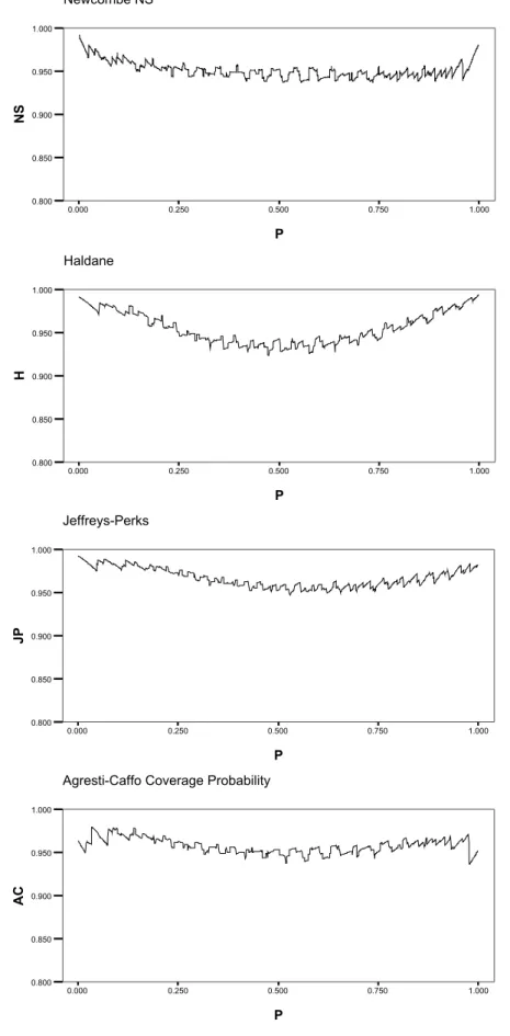
Figure 3 shows the 95% confidence interval coverage probability function for the Newcombe NS, Haldane, Jeffreys-Perks, and Agresti-Caffo methods as a function of π1, π1 ∈ [0,1] for n1 =

n2 = 20 and p2 = 0.3. The NS and Agresti-Caffo

methods demonstrate coverage probabilities that are near nominal over π1∈ [0, 1].

Figure 4 shows the 95% confidence interval coverage probability function for the Newcombe NS, Haldane, Jeffreys-Perks, and Agresti-Caffo methods as a function of π1, π1∈

[0,1] for n1 = 20, n2 = 10 and p2 = 0.3. In the

unequal sample size situation, Newcombe NS and Agresti-Caffo coverage probability functions are near nominal over π1∈ [0, 1].

Conclusion

In the case of differences between two independent proportions the Wald-z confidence interval behaves poorly with coverage probabilities below nominal values. Considering the coverage probability criterion, two alternative methods demonstrate superior coverage properties and both are easily programmable. Based on these results, the recommendation is to use either the NS or the Agresti-Caffo methods.

Newcombe, R. G. (1998). Interval estimation for the difference between independent proportions: comparison of eleven methods. Stat Med, 17, 873-890.

Radhakrishna, S., Murthy, B. N., Nair, N. G. K., Jayabal, P., & Jayasri, R. (1991). Confidence intervals in medical research. Indian

212

Jeffreys-Perks, and Agresti-Caffo as a function of p1 when p2=0.3 with n1=n2=20

0.000 0.250 0.500 0.750 1.000 P 0.800 0.850 0.900 0.950 1.000 N S Newcombe NS 0.000 0.250 0.500 0.750 1.000 P 0.800 0.850 0.900 0.950 1.000 H Haldane 0.000 0.250 0.500 0.750 1.000 P 0.800 0.850 0.900 0.950 1.000 JP Jeffreys-Perks 0.000 0.250 0.500 0.750 1.000 P 0.800 0.850 0.900 0.950 1.000 A C

REED

213

Figure 4: Coverage probabilities for nominal 95% Newcombe NS, Haldane, Jeffreys-Perks, and Agresti-Caffo as a function of p1 when p2=0.3 with n1=20, n2=10

0.000 0.250 0.500 0.750 1.000 P 0.800 0.850 0.900 0.950 1.000 N S Newcombe NS 0.000 0.250 0.500 0.750 1.000 P 0.800 0.850 0.900 0.950 1.000 H Haldane 0.000 0.250 0.500 0.750 1.000 P 0.800 0.850 0.900 0.950 1.000 JP Jeffreys-Perks 0.000 0.250 0.500 0.750 1.000 P 0.800 0.850 0.900 0.950 1.000 A C

214

Appendix A: Methods for calculation of confidence intervals for the difference between independent proportions

Sample 1 Sample 2 + a b p1 = a/m − c d p2 = b/n Total m m θ = π1−π2 θ' = p1− p2 Method Formula Wald-z LB=(p1 − p2) − zα/2√ (ac/m3 + bd/n3) UB=(p1 − p2) + zα/2√ (ac/m3 + bd/n3) Wald-c LB=(p1 − p2) − [zα/2√{ac/m3 + bd/n3} + (1/m + 1/n)/2] UB=(p1 − p2) + [zα/2√{ac/m3 + bd/n3} + (1/m + 1/n)/2] Haldane-H LB=θ*−w

UB=θ*+w, where θ*=(θ'+z2_{v(1-2ψ'))/1+z}2_u),

w=[z/(1+z2_{u)]√[u{4ψ'(1-ψ')-θ'}2_{}+2v(1-2ψ')θ'+4z}2_u2_(1-ψ')ψ'+z2_v2_(1-2ψ')2_]

ψ'=(a/m+b/n)/2, u=(1/m+1/n)/4, and v=(1/m − 1/n)/4

Jeffreys-Perks-JP

LB=θ*−w

UB=θ*+w, where ψ' (from Haldane method) is:

ψ'=[(a+0.5)/(m+1)+(b+0.5)/(n+1)]/2

Newcombe-NS

LB=(p1-p2) −δ, where δ=√{(a/m−l1)2+(u2−b/n)2}=zα/2√{l1(1−l1)/m+u2(1−u2)/n}

UB=(p1-p2) + ε, where ε=√{(u1−a/m)2+(b/n−l2)2}=zα/2√{u1(1−u1)/m+l2(1−l2)/n}

l1, l2, u1, u2 are the LB and UB for p1 and p2 using Wilson's score method

Agresti & Caffo

LB = (p1-p2) − zα/2√ (ac/m3 + bd/n3)