Analysis of Basic Actuarial Theory for Fixed Premium Variable Benefit Life Insurance

(1)

IV

Analysis of Basic Actuarial

Theory for Fixed Premium

Variable Benefit Life Insurance

John C. Fraser, Walter N. Miller, and Charles M. Sternhell

Abstract

This paper presents an analysis of the basic actuarial theory for life insurance policies which have (1) fixed premiums, (2) the entire reserve held in a separate account, the assets of which would be invested primarily in common stocks, and (3) benefits adjusted to reflect the investment performance of the separate account in such a manner that the policyowners would bear the entire investment risk and the life insurance company would not share any part of the investment risk. Policies satisfying these three basic objectives are referred to as fixed premium variable benefit policies.

Face amounts under such policies are adjusted by a simple method that satisfies the requirement that the reserve per dollar of actual face amount at the end of each policy year for a fixed premium variable benefit policy be exactly the same as that for a corresponding fixed benefit policy. It is shown that the actual face amount applicable at the end of any policy year is equal to the actual face amount applicable at the end of the preceding policy year multiplied by a Y factor, representing the adjustment to reflect the fact that a fixed premium is payable, and a Z factor, representing the adjustment to reflect the relationship between the actual net annual investment return on the separate account during the policy year and the interest rate assumed in the calculation of net annual premiums and reserves.

There is no need to change present statutory minimum nonforfeiture and reserve standards in order to

accommodate fixed premium variable benefit policies as long as such standards are interpreted as being applicable per dollar of actual face amount. Similarly, cash surrender and nonforfeiture values per dollar of actual face amount can be illustrated in policy forms for these policies in exactly the same way as those presently illustrated for regular fixed benefit policies. Some other problem areas that are discussed are grace period, reinstatement, policy loans, dividend options, and settlement options.

The paper clearly indicates that it is possible to develop actuarially sound fixed premium variable benefit life insurance policies. These policies would offer the public the opportunity of buying a life insurance product that reflects the investment performance of reserves invested in equities but that has practically all the char- acteristics of regular fixed benefit life insurance policies. The paper was written in order to stimulate the enactment of appropriate legislation that would be suffi- ciently broad to permit the introduction of fixed premium variable benefit policies and of equity-based variable life insurance policies that reflect various alternative approaches.

I. Introduction

The authors of this paper were assigned the problem of determining the kind of variable life insurance policy that they would recommend if there were no statutory or regulatory problems to take into account at either the

(2)

state or federal level. This paper presents the results of some of the basic actuarial research that was done at the New York Life Insurance Company in connection with this problem.

The first step in this research consisted of a review of all the available literature describing the different types of variable life insurance policies that have been introduced in foreign countries, where life insurance compa- riles do not face the same statutory and regulatory problems that they do in the United States. After a thorough review of this literature, the authors agreed that they were not completely satisfied with any of the variable life insurance products currently being sold in other countries.

It was then decided to approach this problem on a purely theoretical basis, keeping in mind the following basic objectives:

1. An attempt would be made to develop the basic actuarial theory for life insurance policies with variable benefits and with fixed premiums.

2. The life insurance company would hold the reserves for these life insurance policies in a separate account, the assets of which would be invested primarily in common stocks.

3. The benefits payable under these life insurance policies would be appropriately adjusted to reflect the investment performance of the separate account, so that the policyowners would bear the entire investment risk with respect to the investment performance of the separate account and the life insurance company would not share any part of this investment risk.

It should be noted that the basic actuarial theory for variable life insurance policies, under which all premiums and benefits are expressed in terms of units instead of dollars, is, of course, exactly the same as the basic actuarial theory for corresponding fixed dollar life insurance policies, under which all premiums and benefits are expressed in terms of dollars. The basic problem with this type of variable life insurance policy is the fact that premiums would have to vary in accordance with variations in the unit value of the separate account.

As far as the authors could determine, nothing has yet been published with respect to the basic actuarial theory underlying variable benefit life insurance policies under which fixed premiums (in terms of dollars) are payable, the entire reserve is invested in a separate account, and the benefits vary to reflect the investment

performance of the separate account in such a manner that the life insurance company does not share any part of the investment risk. The basic actuarial theory for variable life insurance policies of this type (hereinafter referred to as "fixed premium variable benefit" policies) is developed in Section II of this paper.

Section III discusses the changes required in the basic actuarial concepts underlying the standard valuation and nonforfeiture laws in order to accommodate fixed premium variable benefit policies.

Section IV discusses the policy-form problems involved in illustrating actual cash-surrender values and nonforfeiture benefits for fixed premium variable benefit policies.

Section V discusses some other areas where changes in existing statutory requirements would be desirable in order to accommodate fixed premium variable benefit policies. The specific areas discussed are grace period, reinstatement, policy loans, dividend options, and settlement options.

Section VI discusses some possible variations in the basic concepts underlying fixed premium variable benefit policies. The particular variations discussed are a combination of fixed benefits and variable benefits in the same policy, options to vary premiums within pre- scribed limits, and guarantee of minimum benefits for appropriate extra premium.

Section VII presents the conclusion.

This paper does not cover any of the possible regulatory requirements that may be introduced at the federal level by the Securities and Exchange Commission in connection with fixed premium variable benefit policies.

The authors wish to express their appreciation for the valuable contributions that were made by Harold Cherry, ES.A., and R. Stephen Radcliffe, A.S.A., in connection with the preparation of this paper.

II. Development of Basic Actuarial

Theory

Our objective in this section is to develop a method for determining the death benefits under a fixed premium variable benefit life insurance policy which will result in the entire investment risk being borne by the policyowners.

(3)

Basic Theory

for

Fixed Premium

Variable Benefit Life Insurance Policy

Using Traditional Assumptions

In order to illustrate the basic concepts as simply as possible, we will first consider a level annual premium whole life insurance policy using traditional functions, that is, with premiums payable at the beginning of the policy year and death benefits payable at the end of the policy year of death.

We begin with the familiar equation of equilibrium showing the relationship between successive terminal reserves under a fixed premium fixed benefit whole life insurance policy for a face amount of $1.

( , _ , V ~ + P ~ ) ( I + i ) = q , + , _ , ( 1 - , V x ) + , V , , (1) where

t_lVx

Px=

i = q x + t - I ~" tVx

Terminal reserve at the end of policy year t - 1 for a whole life policy issued at age x. Net level annual premium for a whole life policy issued at age x

Interest rate assumed in the calculation of the net annual premium and reserves. Rate of mortality at attained age x + t - 1. Terminal reserve at the end of policy year t for a whole life policy issued at age x. Let us now consider a fixed premium variable benefit whole life insurance policy with an initial face amount of $1 and with the same fixed net level annual premium as that for the corresponding fixed premium fixed benefit whole life insurance policy. Let us assume that the reserves for this policy will be invested in a separate account and that the face amount of this policy will be adjusted annually to reflect the investment performance of the separate account, so that the entire investment risk is borne by the policyowners. We will further require that the reserve per $1 of face amount at the end of each policy year for the fixed premium variable benefit whole life insurance policy be the same as that for the corresponding fixed premium fixed benefit whole life insurance policy. The counterpart of equation (1) for a policy of this type is

[F,_, (,_iV,) +P~ 1(1 + i: ) =

q,+,_,[F,-F,C,V~)] +F,(,Vx) , (2)

where

i~ = Actual net annual investment return on

the separate account during the tth policy year, including realized and unrealized appreciation and depreciation. Ft_ l and F, = Face amounts at the end of the (t - 1)st

and tth policy years, respectively. It should be noted that the initial face amount Fo = 1.

Equation (2) can be rewritten as follows: [F,_, (,_, V~) +P, 1(1 + i; ) =

F,[q~+,_,(1 -tV~) + ,V~]. (3) The expression in brackets on the right side of equation (3) can be seen, by referring to equation (1), to be equal to (,_,Vx +P~ )(1 + i). Substituting in equation (3), we obtain

[F,,_, (,_, V,) + P , ] ( 1 + i~ ) =

F,[(,_,Vx +P~)(1 + i ) ] . (4) Solving for F,, we obtain

= v.Ft_L (,.:2 V~_.~) + P~ ](1 + i~

F, L t-l Vx + Px J k , ' l ~ J'

(5)

which can be rewritten as

(,_,V~ + Px/F,_,.~(1 + i : ~

F, = F,_I k ,_IVx+Px J k l + i j " (6) It is seen that the face amount F, at the end of policy year t can be obtained by multiplying the face amount Ft_ ~ at the end of policy year t - 1 by two factors, which we will call Y, and Z,, where

y, = ,_ ,V~ + P J F , _ , ; (7) t- tVx + Px

1+i~

z , = ~ ( 8 )

1 + i

Thus, in terms of these factors we have

F, = F,_, Y,Z,. (9)

It can be seen that the determination of the actual face amounts under a fixed premium variable benefit

(4)

policy involves the use of a recursion process. Thus, for the first policy year, we have

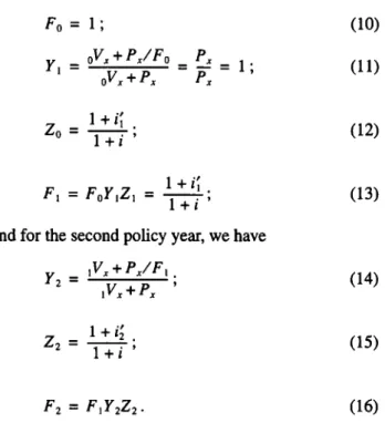
Fo = 1 ; (10) El - OV~ + P J F o = P~-- = 1 ; (11) 0V~+ P~ P~ Z o - l + i ~ . (12) 1 + i ' FI = FoYlZl = l + i ~ . 1 + i ' (13)

and for the second policy year, we have

Y2 = 1V~+ P x / F t ; (14)

iVx+ Px

Z2 = 1 + i._....~., (15)

1 + i

F2 = FIY2Z2. (16)

To obtain the face amounts for the third and subsequent policy years, the process is continued, making repeated use of equations (7), (8), and (9).

While the above development was for a whole life policy, it should be apparent that the derivation can be readily extended to any of the standard forms of insurance, such as term, endowment, and limited payment life plans. Furthermore, the derivation can be extended to (a) plans in which the net premiums are not level but the dollar amount of each net premium is determined in advance in accordance with a specified schedule (e.g., a modified whole life plan or a plan under a modified reserve method) and (b) plans in which the face amount under the corresponding fixed benefit policy varies from year to year in accordance with a specified schedule.

Note that after a policy becomes paid up ,_ iV + O/F,_ 1 t- iV

Y , - - = 1, (17)

, _ i V + 0 ,_iV

and the face amounts change each year only according to the Z, factors.

Illustrative Results

Table 1 illustrates the calculation of face amounts o f insurance for the first three policy years under a fixed premium variable benefit whole life policy with an initial face amount of $1,000 issued to a male age 55, under various levels of investment performance. The net level annual premium and the reserves are based on the 1958 C.S.O. Table, 3 per cent interest, and traditional functions. Illustrative calculations are shown for constant net annual investment returns of 0, 3, 6, and 9 per cent on the separate account, including realized and unrealized appreciation and depreciation.

Table 2 summarizes the results of calculations similar to those in Table 1 carded out to the last age o f the mortality table. The columns headed "Constant" show the face amounts of insurance if actual investment performance were at the rates indicated for every policy year.

O f course, under realistic market conditions the rate would fluctuate considerably over the term of the policy. In order to reflect realistic conditions, a simulation program written in FORTRAN IV for the IBM 1130 computer was developed to produce stock market cycles which resemble what happens in the real world. The simulated stock market performance was developed as the product of three factors:

1. A trend factor, which is simply a regular interest accumu- lation at the assumed underlying net annual investment retBrll.

2. A cycle factor, which behaves like the market cycles found in the real world and varies randomly for each simulation. 3. A random factor, which is independent of the trend or

cycle factors.

The cycle and random factors were designed so that their effect tends to average 100 per cent over a given simulation.

The results under simulated market conditions, based on underlying net annual investment returns of 0, 3, 6, and 9 per cent, are shown in Table 2 under the columns headed "Simulated" It should be understood that the results presented here relate to a single simulation for each underlying net annual investment return with a trend factor based on the rate indicated and that these results do not represent the average of a large number o f such simulations.

(5)

TABLE 1

ILLUSTRATIVE CALCULATIONS FOR FIRST T H R E E P O L I C Y YEARS FOR FIXED PREMIUM VARIABLE BENEFIT W H O L E L I F E POLICY WITH INITIAL FACE AMOUNT OF $ 1 , 0 0 0 ISSUED TO A M A L E A G E 55

(Net Level P r e m i u m s and Reserves Based on 1958 C.S.O. Table, 3 Per Cent Interest, and Traditional Functions)

Net Annual Investment Performance o f Separate Account

• P . 0 . t . r

~, = 0% I ~, = 3% ~, = 6%'

I

t, = 9%

1. Net level annual premium per

$1,000

... 2. Initial face amount = 1,000 F 0 ... 3 . 1 , 0 0 0 (1) + (2) ... 4. Terminal reserve per $1,000 end o f prior year ... 5. (3) + (4) ... 6. (1) + (4) ... 7. Factor Yj = (5) + (6) ... 8. Factor Z~ = (1 + i~ ) + 1.03 ... 9. Face amount under fixed premium variable benefit

policy = 1,000 F I = 1,000 F 0 YI Zi = (2) (7) (8) ...

1. Net level annual premium per $1,000 ... 2. Face amount end o f prior year = 1,000 F~ = (9)pr

$ 39.09 1,000 39.09 0 39.09 39.09 1.0000 0.9709 971 $ 39.09 971

First

Policy

Year

$ 39.09 1,000 39.09 0 39.09 39.09 1.0000 1.0000 1,000 $ 39.09 1,000 39.09 0 39.09 39.09 1.0000 1.0291 1,029 Second PolicyYear 3 . 1 , 0 0 0 (1) + (2) ... 4. Terminal reserve per $1,000 end of prior year ... 5. (3) + (4) ... 6. (1) + (4) ... 7. Factor Y2 = (5) + (6) ... 8. Factor Z 2 -- (1 + it ) + 1.03 ... 9. Face amount under fixed premium variable benefit

policy= 1,000 F 2 = 1,000 F I Y2 Z2 = (2) (7) (8) ...

1. Net level annual premium per $1,000 ...

40.26 27.62 67.88 66.71 1.0175 0.9709 959 $ 39.09 1,000 $ 39.09 1,029 37.99 27.62 65.61 66.71 0.9835 1.0291 $ 39.09 1,000 39.09 0 39.09 39.09 1.0000 1.0583 1,058

2. Face amount end o f prior year = 1,000 F 2 = (9)0 r . ... 3 . 1 , 0 0 0 (1) + (2) ... 4. Terminal reserve per $1,000 end o f prior year ... 5. (3) + (4) ... 6. (1) + (4) ... 7. Factor Y3 = (5) + (6) ... 8. Factor Z 3 = ( 1 + i'3 ) + 1.03 ... 9. Face amount under fixed premium variable benefit

policy = 1,000 F~ = 1,000 F 2 Y3 Z~ = (2) (7) (8) ... $ 39.09 1,058 36.95 27.62 64.57 66.71 0.9679 1.0583 39.09 27.62 66.71 66.71 1.0000 1.0000 1,000 1,041 1,084

Third Policy Year

$ 39.09 $ 39.09 $ 39.09 ] $ 39.09 1,084 36.06 55.28 91.34 94.37 0.9679 1.0583 1,110 959 40.76 55.28 96.04 94.37 1.0177 0.9709 948 1,000 39.09 55.28 94.37 94.37 1.0000 1.0000 1,000 1,041 37.55 55.28 92.83 94.37 0.9837 1.0291 1,054

(6)

TABLE 2

ILLUSTRATIVE FACE AMOUNTS FOR FIXED PREMIUM VARIABLE BENEFIT WHOLE LIFE POLICY WITH INITIAL FACE AMOUNT OF $1,000 ISSUED TO A MALE AGE 55

(Net Level Premiums and Reserves Based on 1958 C.S.O. Table, 3 Per Cent Interest, and Traditional Functions) NET ANNUAL INVESTMENT PERFORMANCE OF SEPARATE ACCOUNT

End of

Policy i' - 0% ~ i' = 3% i' = 6% i' = 9%

Year

Simulated Constant Simulated

. . . . . . . . . . . . . . . o o . . . o o . . . . . . o , . . . o ° 10 ... 11 ... 12 ... 13 ... 14 ... 15 ... 16 ... 17 ... 18 ... 19 ... 20 ... 21 ... 22 ... 23 ... 24 ... 25 ... 26 ... 27 ... 28 ... 29 ... 30 ... 31 ... 32 ... 33 ... 34 ... 35 ... 36 ... 37 ... 38 ... 39 ... 0 . . . 41 ... 42 ... 43 ... 4 . . . 45 ... Constant $971 $ 968 959 991 948 1,036 937 838 926 846 915 888 904 909 893 812 883 908 873 881 863 904 853 876 843 820 834 811 825 797 816 ! 974 807 873 799 716 791 802 783 775 767 760 753 746 739 732 725 719 713 707 701 695 690 685 680 675 670 665 660 655 650 645 640 635 782 831 806 833 863 737 732 617 723 733 819 793 651 667 706 727 704 600 667 629 698 693 695 587 563 722 Constant Simulated $1,000 $1,035

1,000

1,070

1,000 904 1,000 908 1,000 920 1,000 1,059

1,000

1,068

1,000 1,030 1,000 924 1,000 841

1,000

981 1,000 976 1,000 1,138 1,000 1,047 1,000 988

1,000

1,057

1,000

1,030

1,000 898

1,000

1,090

1,000 877 1,000 1,131 1,000 950

1,000

1,112

1,000 952 1,000 1,028

1,000

1,008

1,000 927

1,000

1,078

1,000

1,050

1,000 1,046 1,000 987

1,000

1,080

1,000 959

1,000

1,030

1,000.

1,064

1,000

1,032

1,000

1,043

1,000 969

1,000

1,055

1,000 910 1,000 1,026

1,000

1,064

1,000 970 1,000 947

1,000

1,070

Constant Simulated $1,029 $1,043 1,041 943 1,054 1,145 1,067 1,100 1,080 1,174 1,093 960 1,106 991

1,120

1,097

1,134 1,229 1,148 967 1,162 1,245 1,177 1,260 1,192 1,194 1,207 1,220 1,222 1,220 1,237 1,288 1,252 1,420 1,268 1,293 1,284 1,305 1,300 1,162 1,316 1,396 1,332 1,114 1,348 1,398 1,364 1,400 1,381 1,630 1,398 1,587 1,415 1,512 1,432 1,396 1,449 1,325 1,466 1,519 1,483 1,275

1,500

1,619

1,517 1,429 1,535 1,565 1,553 1,591 1,571 1,750 1,589 1,503 1,607 1,584 1,625 1,704 1,643 1,735 1,662 1,576 1,681 1,546 1,700 1,532 1,720 1,835 1,740 i 1,959 $1,058 1,084 1,110 1,137 1,165 1,194 1,224 1,255 1,287

1,320

1,355 1,391 1,428 1,466

1,505

1,545 1,586 1,628 1,672 1,717 1,763 1,811

1,860

1,911 1,963 2,016 2,071 2,128 2,186 2,245 2,306 2,369 2,433 2,499 2,567 2,637 2,709 2,783 2,859 2,937 3,018 3,102 3,189 3,279 3,373 $1,086 1,021 1,152 1,033 1,257 1,264 1,231 1,185 1,136 1,391 1,209 1,511 1,478

1,580

1,536 1,717 1,600 1,597 1,494 1,704 1,741 1,797 1,668 2,042 2,030 2,072 2,260

1,808

1,839 2,322 2,410 2,422 2,519 2,088 2,608 2,857 2,492 2,889 2,993 3,054 2,533 3,068 3,755 3,488 2,973

(7)

TABLE 3

ILLUSTRATIVE FACE AMOUNTS FOR FIXED PREMIUM VARIABLE BENEFIT POLICIES WITH INITIAL FACE AMOUNT OF $1,000 ISSUED IN JULY,

1915,

WITH SEPARATE ACCOUNT INVESTED IN STANDARD AND POOR'S COMPOSITE

500

(Net Level Premiums and Reserves Based on 1958 C.S.O. Table, 3 Per Cent Interest, and Traditional Functions)

Policy Year Whole Life 20-Pay Life 20-Year Endowment

Ending in:

Age 25 at Issue Age 55 at Issue Age 25 at Issue Age 55 at Issue Age 25 at Issue Age 55 at Issue 1916 ... 1917 ... 1918 ... 1919 ... 1920 ... 1921 ... 1922 ... 1923 ... 1924 ... 1925 ... 1926 ... 1927 ... 1928 ... 1929 ... 1930 ... 1931 ... 1932 ... 1933 ... 1934 ... 1935 ... 1936 ... 1937 ... 1938 ... 1939 ... 1940 ... 1941 ... 1942 ... 1943 ... 1944 ... 1945 ... 1946 ... 1947 ... 1948 ... 1949 ... 1950 ... 1951 ... 1952 ... 1953 ... 1954 ... 1955 ... $1,179 1,075 936 1,246 1,021 869 1,192 1,139 1,296 1,594

1,790

2,115 2,629 3,752 2,657

1,700

782 1,321 1,146 1,469 2,080 2,200 1,625 1,574 1,356

1,402

1,200

1,672 1,836 2,123 2,588 2,271 2,306 2,230 2,700 3,457 3,973 3,911 4,922 6,921 $1,179 1,066 928 1,243 1,010 861 1,190 1,130 1,281 1,565 1,738 2,028 2,484 3,484 2,416 1,522 696 1,199 1,039 1,336 1,884 1,970 1,438 1,385 1,187 1,226 1,048 1,464 1,598 1,834 2,213 1,917 1,926 1,843 2,209 2,793 3,162 3,061 3,792 5,239 $1,179 1,078 939 1,248 1,025 872 1,194 1,142 1,300 1,601 1,802 2,135 2,662 3,811 2,709 1,738 801 1,349 1,170

1,500

2,153 2,326 1,755 1,724 1,504 1,568 1,355 1,897 2,108 2,469 3,053 2,722 2,803 2,748 3,370 4,377 5,110 5,111 6,532 9,333 $1,179 1,069 931 1,244 1,014 863 1,190 1,133 1,286 1,575 1,756 2,059 2,538 3,585 2,509 1,591 729 1,243

1,078

1,384 1,987 2,147 1,620 1,591 1,388 1,447

1,250

1,750

1,945 2,278 2,817 2,511 2,586 2,535 3,109 4,038 4,714 4,714 6,025 8,609 $1,179 1,081 942 1,250 1,029 875 1,196 1,145 1,304

1,607

1,811 2,149 2,685 3,853 2,746 1,765 814 1,369 1,188 1,522 $1,179 1,071 932 1,245 1,016 865 1,191 1,135 1,289

1,580

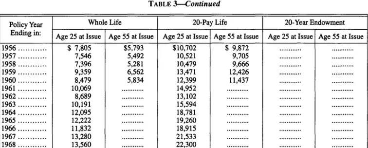
1,765 2,075 2,565 3,637 2,557 1,627 747 1,268 1,100 1,412

(8)

TABLE 3

Continued

Ending in:

Age 25 at Issue Age 55 at Issue Age 25 at Issue Age 55 at Issue Age 25 at Issue Age 55 at Issue 1956 ... 1957 ... 1958 ... 1959 ... 1960 ... 1961 ... 1962 ... 1963 ... 1964 ... 1965 ... 1966 ... 1967 ... 1968 ... $ 7,805 7,546 7,396 9,359 8,479 10,069 8,689 10,191 12,095 12,222 11,832 13,280 13,560 $5,793 5,492 5,281 6,562 5,834 $10,702 10,521 10,479 13,471 12,399 14,952 13,102 15,594 18,781 19,260 18,915 21,533 22,300 $ 9,872 9,705 9,666 12,426 11,437

It is interesting to see what the results would have been for fixed premium variable benefit policies under actual market conditions over a long period of time, if such policies had been issued in the past. Accordingly, in Table 3 we have illustrated the face amounts of insurance under hypothetical fixed premium variable benefit policies issued in July, 1915, if the separate account had been fully invested in common stocks experiencing the performance level (including dividend yields) of Stan- dard and Poor's Composite 500. Results are illustrated for whole life, twenty-pay life, and twenty-year endowment policies issued to a male at ages 25 and 55.

Based on the performance of the stock market over the last fifty-odd years, the results under the hypothetical fixed premium variable benefit policies shown in Table 3 are quite dramatic, especially for policies in force at the longer durations. For the two policies which could possibly be in force in 1968--the whole life and twenty-pay life policies issued at age 25--the face amount in 1968 is over 13 times the initial face amount of $1,000 for the whole life policy and over 22 times the initial face amount for the twenty-pay life policy. There are only occasional points during the period of coverage in this particular illustration where the face amount drops below the initial face amount of $1,000.

In order to illustrate results under rather adverse market conditions, Table 4 shows what would have hap- pened if fixed premium variable benefit policies similar to those illustrated in Table 3 had been issued in August, 1929, just prior to a major stock market crash. It will be noted that for all but a few of the years from issue to 1942 the face amounts are less than the initial face amount of $1,000. However, from 1943 on, the face amounts exceed $1,000, reaching the $5,700- $12,500 range in 1968 for the plans and issue ages illustrated.

Alternative Unit Value Approach

It is, of course, possible to express the basic actuarial theory underlying a fixed premium variable benefit life insurance policy in an alternative manner by using number of units of face amount and unit values of the separate account in which the reserves are invested.

Let

u 0 = Unit value of separate account on the effective date of the policy;

u, = Unit value of separate account at the end of the tth policy year.

(9)

TABLE 4

ILLUSTRATIVE FACE AMOUNTS FOR FIXED PREMIUM VARIABLE BENEFIT POLICIES WITH INITIAL FACE AMOUNT OF $1,000 ISSUED IN AUGUST,

1929,

WITH SEPARATE ACCOUNT INVESTED IN STANDARD AND POOR'S COMPOSITE

500

(Net Level Premiums and Reserves Based on 1958 C.S.O. Table, 3 Per Cent Interest, and Traditional Functions)

Ending in:

Age 25 at Issue Age 55 at Issue Age 25 at Issue I Age 55 at Issue Age 25 at Issue Age 55 at Issue 1930 ... 1931 ... 1932 . . . 1933 ... 1934 ... 1935 ... 1936 ... 1937 ... 1938 ... 1939 ... 1940 ... 1941 ... 1942 ... 1943 ... 1944 ... 1945 ... 1946 ... 1947 ... 1948 . . . 1949 . . . 1950 ... 1951 ... :1952 ... 1953 ... 1954 ... 1955 1956 . . . 1957 . . . 1958 . . . 1959 . . . 1960 ... 1961 ... 1962 ... 1963 ... 1964 ... 1965 ... 1966 ... 1967 . . . 1968 . . . $ 682 569 467 821 717 960 1,371 1,337 1,008 943 916 929 820 1,169 1,286 1,559 1,654 1,516 1,592 1,541 1,901 2,434 2,631 2,460 3,153 4,516 4,898 4,611 4,823 5,907 5,535 6,495 5,550 6,684 7,403 7,738 6,735 8,059 8,370 682 58O 485 871 754 1,011 1,431 1,374 1,023 955 927 942 832 1,191

1,303

1,567 1,645 1,491 1,552 1,489 1,822 2,306 2,456 2,261 2,858 4,026 4,282 3,952 4,056 4,873 4,474 5,147 4,308 5,090 5,524 5,657 4,823 5,660 5,760

L

$ 682 ' $ 565 460 804 704 943 1,349 1,321 999 936 909 922 814 1,159 1,277 1,550 1,648 1,514 1,593 1,545 1,936 2,528 2,797 2,676 3,503 5,135 5,711 5,510 5,899 7,388 7,081 8,489 7,410 9,104 10,287 10,967 9,730 11,856 12,539 682 577 479 855 742 995 1,413 1,364 1,020 953 925 939 829 1,184 1,298 1,567 1,654 1,507 1,576

1,520

1,904

2,486 2,750 2,631 3 ,A. A. A . 5,048 5,614 5,416 5,798 7,262 6,961 8,345 7,284 8,949 10,111 10,779 9,563 11,653 12,324 $ 682 562 455 791 693 928 1,330 1,306 990 928 902 915 808 1,150 1,268 1,541 1,641

1,509

1,589 1,543 $ 682 575 476 847 736 986 1,402 1,358 1,018 951 923 937 827 1,180 1,295 1,566 1,656 1,513 1,586 1,533

(10)

Let us assume that unit values of the separate account are adjusted to reflect the actual net investment return on the separate account (i.e., i~ during the tth policy year) in relation to the interest rate of i assumed for the calculation of net annual premiums and reserves, so that

(1 + i~

"~. ~l ~-" UO t'~'-@'=~) , ( 1 8 )

(1

+i~'~

Ut -m- Ut_lt--i-~l ) • (19) Now, let

X 0 = Initial number of units of face amount; X, = Number of units of face amount at the end of

the tth policy year.

Let us now consider a fixed premium variable benefit whole life insurance policy with an initial face amount of $1 and with a fixed net level annual premium of P~. The initial face amount can be expressed as $1 = F o =

Xou o.

The face amount at the end of the (t - 1)st policy year can be expressed as

Ft_ I = Xt_lUt_l, (20)

and the face amount at the end of the tth policy year can be expressed as

F, = X,u r

(21)

Substituting equations (20) and (21) in equation (6), we obtain

:,_,Vx +

Px/X,_iu,_,~(1

+

i't

X,u, = X,_lU,_l|

(22)

t _ l V x + P x ) k l + i ) "

\

Substituting the value of u, from equation (19) in equation (22), we obtain

i'

.. ( 1 + ,~ J t t U t - l t ~ ) ~" X .t ( t _ l V x + P x / t_lUt_i'~(m + lt'~

X,_,U,_l(..

",-IV-~+-~

" ) t . ~ ) "

(23)

Dividing both sides of equation (23) by u,_~[(1 + i; ) / ( 1 + i)1, we obtain

¢t- iVx + e x / X t - l•t - 1"~

x, = x,_, L

+ E

2"

(24)

Equation (24) defines the recursion process required to determine the change in number of units from the end of the (t - 1)st policy year to the end of the tth policy year under a fixed premium variable benefit policy. It should be noted that this change in number of units actually takes place at the beginning of the tth policy year when the net annual premium Px is placed in the separate account and reflects the fact that a fixed premium is payable under this policy. In order to keep the number of units of face amount constant from year to year, premiums would have to vary in accordance with variations in the unit values of the separate account.

If equations (20) and (24) are referred to, it can be seen that the number of units of face amount will decrease at the beginning of the tth policy year if

F,_

1 = X t - i u , _ 1 is greater than 1. On the other hand, the number of units of face amount will increase at the beginning of the tth policy year if F,_ ~ =

X,_ ~ u,_ ~

is less than 1.

C o m p a r i s o n o f Two M e t h o d s

The complete symmetry between the two methods of analyzing the basic actuarial theory underlying a fixed premium variable benefit policy can now easily be dem- onstrated. Substituting F,_~ for

X,_~U,_l

in equation (24), we obtain

(t-lVx + Px/F,-~)

(25)

X, = Xt-t

t-IV~+Px

"

Referring to equation (7), we can see that the expression in parentheses in equation (25) is equal to Y,. Sub- stituting, we obtain

X, = X,_

I Y, ; (26)

X, (27)

Y' = X,_I"

Referring to equations (8) and (19), we can see that

u, = u,_lZ, ; (28)

Z, = u, (29)

U i _ l "

The roles of the Y, and

Z,

factors in the basic equation (9), that is,

F, = F,_~ Y,Z,,

(9)

can now be clearly expressed as follows:.

(11)

a) The role of the Y, factor is to adjust the number of units of face amount (and hence the face amount) at the beginning of the tth policy year to reflect properly the fact that a fixed premium of P~ is payable at that time.

b) The role of the Z, factor is to adjust the face amount so as to reflect the effect of the change in unit values from the beginning of the tth policy year to the end of the tth policy year.

It should be noted, however, that there is no need to refer to number o f units or unit values in determining actual face amounts under a fixed premium variable benefit policy. Actual face amounts under such a policy can be determnined solely from the Yt and Z t factors defined in equations (7) and (8).

Extension of Basic Theory to Policy with

Net Annual Premiums and Reserves

B a s e d on C o n t i n u o u s F u n c t i o n s

Thus far we have considered a fixed premium variable benefit policy where the net annual premiums and terminal reserves are based on traditional functions. Formulas analogous to equations (7), (8), and (9) for determining the face amounts under a fixed premium variable benefit policy with net annual premiums and reserves based on continuous functions are presented below.

We will once again use a whole life policy to illustrate the basic formulas. The two bases for net annual premiums and terminal reserves using continuous functions commonly found in practice follow:

a) A "semi-continuous" basis, where the net annual premium is

t'(,4~) = '4~..--

ax

and the terminal reserve at the end of the tth policy year is

**,v(~,) = * , . , - e ( ~ , ) a x ÷ , .**

b) A "fully continuous" basis, where the net annual premium is

and the terminal reserve at the end of the tth policy year is

Both of the above bases reflect the assumption that the face amount is payable at the moment of death. Thus it is apparent that the face amount payable at death under a fixed premium variable benefit policy with net annual premiums and reserves calculated on basis (a) or (b) should vary continuously during the policy year in accordance with the net investment performance o f the separate account from the beginning of the policy year to the moment o f death.

Consider first a fixed premium variable benefit whole life policy where net annual premiums and reserves are calculated on basis (a) described above. Let F~_ i be the face amount payable at the end of the (t - 1)st policy year and F~_~+: be the face amount payable a fraction of a year f later. It can be shown that if we define Y and Z factors as follows:

y~ = ,_,V(A~) + P(A~)/FT_~ ,_ ~V(A~) + P(,4~) ' (30) . i 1 + st-i:/ Z~-~:I = 0 < f < l , (31) (i + i) / '

where i~_ ~:/ is the actual net investment return from the beginning of the tth policy year to a fraction of a y e a r f l a t e r (i.e., to the moment of death), then

a Ft-I a Y, t-~:f , a Z a

F t - t ÷ : = 0 < f < l (32)

b

Similarly, under basis (b), let F,_~ be the face amount payable under a fixed premium variable benefit whole life policy at the end o f the (t - 1)st policy year and _{F,_ 1 +: be the face amount payable a fraction o f a}b year f later. Then, if we define Y and Z factors as follows: yb = ,-,V(A~)_ +_[(d/8)P(Ax)]/F~_, , (33) ,_,V(Ax) + ( d / 5 ) e ( A ~ ) 1 + "" Z~_ t:: = t,_ i:: 0 < f < 1, (34) (I + i) / '

it can be shown that

b b b b

F,-1 Y, Z , - l . /

F t - l + / =

It will be noted that

Z , L ~:: = Z, ~_, : .

0 < f < 1. (35)

(12)

As is true in the case of traditional functions, the above formulas were derived on the assumption that the reserve per $1 of face amount at the end of each policy year for the fixed premium variable benefit whole life policy is the same as that for the corresponding fixed premium fixed benefit whole life policy.

III. Changes Required in Basic

Actuarial Concepts Underlying

Standard Valuation and

Nonforfeiture Laws

The basic actuarial concept underlying a fixed premium variable benefit policy is that the face amount of the policy is adjusted to reflect the investment performance of a separate account, based on the assumption that reserves for this policy are held in the separate account. The particular method of adjusting the face amount that was derived in Section II involved the additional requirement that the reserve per dollar of face amount at the end of each policy year for a fixed premium variable benefit policy be exactly the same as that for a corresponding fixed premium fixed benefit policy. Keeping this relationship in mind, we will analyze the basic actuarial concepts underlying the standard valuation and nonforfeiture laws in order to determine what changes are required in these concepts in order to accommodate a fixed premium variable benefit policy.

Standard Valuation Law

The basic concept underlying the standard valuation law is to provide a test for solvency by specifying the minimum reserve standards that life insurance companies can use in calculating the reserves they are required to hold in order to provide for future liabilities in connection with their in-force life insurance policies. Thus, for individual life insurance policies, the present statutory minimum reserve standards involve a conservative mortality table, a maximum interest rate, and a prospective valuation method.

In considering the application of this concept to fixed premium variable benefit policies, let us first examine the net level annual premium reserves for such policies from a prospective standpoint, using the particular assumption that future investment performance of the separate account will be at the assumed interest rate i

used for calculation of net annual premiums and reserves. Under this assumption, the net level annual premium reserve for a fixed premium variable benefit whole life policy at duration t will reflect future face amounts Ft÷l, /7,+ 2 .. . . . which can be calculated using formulas (7), (8), and (9) given in Section II of this paper. (Note that all Z , factors are equal to 1 under the assumption that actual net annual investment performance of the separate account will be at the assumed interest rate i.) These face amounts will not be level except in the special case where F , is equal to the initial face amount.

Therefore, the present value of future benefits can be expressed as

1 o - x - t - I

A~+, = Dx+, ~ (C . . . . j)(F,+~+,), (36) j = 0

where the commutation functions are computed at the assumed interest rate i and the future face amounts F,+,,

F,+ 2, . . . , are calculated as follows:

F t + j + 1 = F , + j Y , + I + t . (37) The present value of the fixed net level annual premiums Px under the fixed premium variable benefit whole life policy is clearly Pfi~+t, where d~+ t is computed at the assumed interest rate i. The prospective reserve for the fixed premium variable benefit whole life policy is therefore equal to

A '~ + , - P ~ii~ + , . (38)

In Section II, however, it was indicated that the reserve for the fixed premium variable benefit whole life policy can be expressed as F,(,Vx). Since , V x = Ax÷ ~ -

Pfix÷,, it is therefore apparent that

F,(,V) = F,A~+,- F,Pfix÷,. (39) This is also an expression for the prospective reserve on a fixed premium variable benefit whole life policy, and it seems to be quite different from the expression given in equation (38) above. Expression (39) involves a level benefit F, rather than the series of nonlevel benefits defined by equation (37) and a net level annual premium of FtP~ rather than P~.

It is therefore essential to demonstrate that expres- sions (38) and (39) are equivalent, that is, that

A'x+, - P fiix+, = F , ( , V ~ )

= F , A ~ + , - F , P f i i ~ + , . (40)

(13)

A proof o f equation (40) is presented in Appendix A. As also noted in Appendix A, this proof can be general- ized to cover plans generally, rather than just whole life; any assumption as to future investment performance; and reserves computed according to methods other than the net level annual premium method (e.g., the commissioners reserve valuation method).

It can therefore be stated that F,(,V) is, in general, the correct terminal reserve for a fixed premium variable benefit policy, since it automatically takes into account the present values, under any level of actual investment performance, o f the future benefits that will be payable and of the actual fixed net premiums that will be payable, based on the particular interest rate assumption and valuation method chosen. This result is to be expected in light of the fact that the company does not bear any investment risk under a fixed premium variable benefit policy.

Since F,(,V) has been shown to be the correct terminal reserve for a fixed premium variable benefit policy, the question of a proper minimum reserve standard for such policy is essentially the question of a proper standard for ,V. Since this factor is the same under a fixed premium variable benefit policy as that under a corresponding fixed benefit policy it, appears logical that it be subject to the same minimum standard. In this connection, it should be noted that any other approach would mean that, when actual investment performance was at the assumed rate and benefits under a fixed premium variable benefit policy were therefore the same as those under a corresponding fixed benefit policy, the minimum reserve for the fixed premium variable benefit policy would be different from that for the corresponding fixed benefit policy. It seems that any such situation would be quite anomalous.

It therefore appears that there is no need to change present statutory minimum reserve standards in order to accommodate fixed premium variable benefit policies, as long as such standards are interpreted as being applicable per dollar of actual face amount under the fixed premium variable benefit policy.

On the assumption that statutory minimum reserve standards are satisfied, life insurance companies should have the same choice o f assumptions for actual reserves under fixed premium variable benefit policies as they presently have for fixed benefit policies. Such a choice will be important from the standpoint o f product design,

because benefits and reserves under a fixed premium variable benefit policy depend not only on the actual investment performance o f the separate account but also on the reserve assumptions that determine the level and incidence of the net premiums that are deposited in the separate account.

This is illustrated in Tables 5 and 6, which show actual face amounts and terminal reserves under various levels of actual investment performance for a $1,000 initial face amount fixed premium variable benefit whole life policy issued to a male age 55. Reserves and net premiums, based on traditional functions, are computed on the basis of the 1958 C.S.O. table with assumed interest rates o f either 2 ½ or 3 per cent and on either the net level premium method or the commissioners reserve valuation method.

The actual face amounts illustrated in Table 5 indicate the following relationships:

a) For a given mortality basis, reserve method, and actual net investment performance, the lower the assumed interest rate the higher the actual face amount.

b) For a given mortality basis, assumed interest rate, and actual net investment performance, actual face amounts under the commissioners reserve valuation method are higher than those under the net level premium method, if actual investment performance is poorer than that according to the assumed interest rate, and are lower than those under the net level premium method if actual investment performance is better than that according to the assumed interest rate. This reflects the fact that, given the same mortality basis and assumed interest rate, funds (i.e., net premiums) are deposited into the separate account relatively later under the commissioners reserve valuation method than they are under the net level premium method. This is advantageous if actual net investment performance is worse than that assumed but disadvantageous if it is better than that assumed.

The actual reserves, per $1,000 initial face amount, illustrated in Table 6 indicate the following relationships:

a) For a given mortality basis, reserve method, and actual net investment performance, the lower the assumed interest rate the higher the actual reserve.

b) For a given mortality basis, assumed interest rate, and actual net investment performance, it is interesting to note that actual reserves under the commissioners reserve valuation method are not always lower than those under the net level premium method. As illustrated in Table 6, actual reserves under the commissioners reserve valuation method can be higher than those under the net level premium method at the longer policy durations if actual net investment performance is worse than that assumed.

(14)

TABLE 5

ACTUAL FACE AMOUNTS FOR FIXED PREMIUM VARIABLE BENEFIT WHOLE LIFE POLICY WITH INITIAL FACE AMOUNT

OF $1,000 ISSUED TO A MALE AGE 55

(Net Premiums and Reserves Based on 1958 C.S.O. Table, Net Level Premium or Commissioners Reserve Valuation Method, 2½ or 3 Per Cent Interest and Traditional Functions)

Net Annual Investment Performance of Separate

Account i' (Per Cent)

... .... .... End of Policy Year Net Level Premium Method 21/9. Per Cent 3 Per Cent

Commissioners Method 926 873 825 783 746 713 685 66O 635 1,000 1,000

1,000

1,080 1,148 1,222 1,300 1,381 1,466 1,553 1,643

1,740

1,165

1,320

1,505 1,717 1,963 2,245 2,567 2,937 3,373 21/9. Per Cent 5 10 15 20 25 30 35 40 45 5 10 15 20 25 30 35 40 45 5 10 15 20 25 30 35 40 45 5 10 15 20 25 30 35 40 45 937 892 851 815 782 753 728 706 686 1,013 1,023 1,033 1,043 1,053 1,063 1,073

1,082

1,092

1,095

1,177 1,266

1,360

1,461 1,567 1,677 1,793 1,918 1,181 1,356 1,563 1,804 2,086 2,416 2,796 3,237 3,764 $ 947 902 861 824 791 762 737 715 695 1,011 1,021 1,031 1,041 1,051

1

061 1,071

1,078

1,087

1,079

1,158 1,244 1,335 1,432 1,533 1,638 1,747 1,866 1,150 1,315 1,511 1,739 2,004 2,311 2,664 3,072 3,558 3 Per Cent 937 884 836 794 757 724 696 671 646

1,000

1,000 1,000 1,000 1,000

1,000

1,067

1,133

1,204

1,279 1,358 1,439 1,524 1,609 1,701 1,136 1,296 1,461 1,661 1,892 2,157 2,456 2,797 3,200

(15)

TABLE 6

ACTUAL TERMINAL RESERVES FOR FIXED PREMIUM VARIABLE BENEFIT WHOLE LIFE POLICY WITH INITIAL FACE AMOUNT

OF $1,000 ISSUED TO A MALE AGE 55

(Net Premiums and Reserves Based on 1958 C.S.O. Table, Net Level Premium or Commissioners Reserve Valuation Method, 2x/2 or 3 Per Cent Interest and Traditional Functions)

Net Annual Investment Performance of Separate

Account i' (Per Cent) .... .... .... .... End of

Po~cy

Net Level Premium Method 3 Per Cent 128 $ 239 330 401 458 498 528 559 635 138 273 400 512 614 698 771 847 1,000 149 314 488 666 848 1,024 1,197 1,392 1,740 161 361 601 880

1,206

1,568 1,979 2,489 3,373 Commissioners Method 2½ Per Cent 5 10 15 20 25 30 35 40 45 5 10 15 20 25 30 35 40 45 5 10 15 20 25 30 35 40 45 5 10 15 20 25 30 35 40 45 2½ Per Cent $ 135 $ 252 350 428 489 534 568 603 686 146 290 425 547 659 753 837 924

1,092

158 333 521 713 914 1,110

1,308

1,531 1,918 170 384 643 946

1,306

1,712 2,180 2,764 3,764 112 236 339 421 486 533 570 607 695 120 267 406 531 646 743 828 916 1,087 128 303 490 681 880

1,073

1,266 1,484 1,866 136 344 595 888 1,232 1,618 2,060 2,610 3,558 3 Per Cent 107 223 320 396 457 499 532 566 646 114 253 383 499 603 690 764 843 1,000 121 286 461 638 819 992 1,165 1,356 1,701 129 325 559 828 1,141 1,488 1,877 2,358 3,200

(16)

It should be kept in mind, however, that on a per $1,000 actual face amount basis, relationships between reserves computed according to various assumptions and methods for a fixed premium variable benefit policy are exactly the same as those under a corresponding fixed benefit policy, because reserves per dollar of actual face amount under a fixed premium variable benefit policy are the same as those per dollar of face amount under a corresponding fixed benefit policy. This means that, for a given mortality basis and assumed interest rate, reserves based on the commissioners reserve valuation method for a fixed premium variable benefit policy are always lower, per $1,000 actual face amount, than net level premium reserves per $1,000 actual face amount.

Standard Nonforfeiture Law

The basic concept underlying the standard nonforfeiture law is to specify minimum cash-surrender values for life insurance policies. These statutory minimum cash-surrender values may be considered to represent rough approximations to retrospective asset share accu- mulations that reflect the actual incidence of expenses, that is, the significantly higher level of expenses during the first policy year than during subsequent policy years.

Actually, the standard nonforfeiture law defines minimum cash-surrender values prospectively as equal to the present value of future benefits less the present value of future adjusted premiums. Using a whole life policy issued at age x for illustrative purposes, the adjusted premium (AP)s can be expressed as follows:

_ I ~

(AP)~ A~+I~ _ p ~ + _ , (41)

/i~ a~

where A s is the present value at issue of future benefits and I~ is the initial expense deficit specified-in the law. The adjusted premium (AP) x may be considered as the sum of the net annual premium P~ and an additional amount lx/ii~ required to amortize the specified initial expense deficit over the entire premium paying period.

The minimum cash-surrender value ,(MCV) x at duration t for a whole life policy issued at age x is defined in the standard nonforfeiture law as

,(MCV)~ = A~+,- (AP)xti,+,.

(42)

Referring to equation (41), equation (42) can be expressed as follows:

,(MCV) s = A~+,-P~//x+,- (lJii~)?i~+, ; (43) ,(MCV)s = ,V~-( l J iis)ii . . . . (44) If we let ,Us represent the unamortized portion of the initial expense deficit at duration t, we obtain

and

,Us = (Ix/a~)as+, (45)

,(MCV)~ = ,Vs-,U~. (46) In considering the basic problem of how to specify statutory minimum cash-surrender values for a fixed premium variable benefit life insurance policy, it is clear that the reserve part of equation (46) does not present any problem, since it has already been demon- strated that F,(,Vx) represents the appropriate reserve at the end of the tth policy year. The basic problem, therefore, is the definition of the unamortized portion of the initial expense deficit, that is, the definition of the fixed premium variable benefit analogue of ,Ux in equation (46).

After a thorough analysis of various possible methods of handling this basic problem, it appeared to us that, from a practical point of view, one method was far superior to any of the other possible methods. Under the proposed method, the unamortized initial expense deficit per dollar of actual face amount at the end of each policy year for a fixed premium variable benefit policy would be exactly the same as that for a corresponding fixed premium fixed benefit policy. Under this proposed method, the statutory minimum cash-surrender value for a fixed premium variable benefit life insurance policy would be

(F,),(MCV) s = F,(,Vx) - F,(,U). (47) In other words, under the proposed method the statutory minimum cash-surrender value per dollar of actual face amount under a fixed premium variable benefit policy would be exactly the same as the statutory minimum cash-surrender value per dollar of face amount under a corresponding regular fixed benefit policy.

It is apparent that the proposed method of specifying minimum cash-surrender values would be quite easy to implement in the development of appropriate legislation and would not involve the recalculation of presently

(17)

published minimum cash-surrender values, since they would continue to be applicable on a per $1,000 actual face amount basis for a fixed premium variable benefit policy.

Appendix B compares the proposed method of specifying minimum cash-surrender values with several alternative methods that were considered.

Since the method adopted for the definition of statutory minimum cash-surrender values for a fixed premium variable benefit policy will have significant effects on the methods that life insurance companies can adopt for the illustration of actual cash-surrender values and nonforfeiture values in life insurance policy forms, this problem will be considered in Section IV of this paper.

IV. Problems Involved in Illustrating

Actual Cash-Surrender Values

and Nonforfeiture Benefits in

Policy Forms

In this section, we shall examine the problems involved in illustrating cash-surrender values and nonforfeiture benefits in policy forms for a fixed premium variable benefit policy if our proposed method of defining statutory minimum cash-surrender values is adopted.

Extension of the concept underlying our proposed method of defining minimum cash-surrender values would mean that the fixed premium variable benefit policy form could show a table of cash-surrender values per $1,000 of actual face amount. This table would look exactly like the table of cash-surrender values per $1,000 of face amount which appears in a fixed benefit policy.

In similar fashion, the fixed premium variable benetit policy form could show a table of reduced paid-up values per $1,000 of actual face amount which would look exactly like the table of such values per $1,000 of face amount which appears in a fixed benefit policy. The formula used to compute such values under a fixed premium variable benefit policy would also be exactly the same as that used in the case of a corresponding fixed benefit policy. For example, consider the calculation of the reduced paid-up value applicable at the end of policy year t under a fixed premium variable benefit whole

life policy issued at age x for an initial face amount of $1,000. Let us denote the reduced paid-up value per $1,000 of actual face amount to be shown in the policy by ~P,. The actual amount of reduced paid-up insurance would therefore be F,(,RP,). If ,CV, is the cash- surrender value per $1,000 of actual face amount under the fixed premium variable benefit whole life policy at the end of policy year t, the actual cash-surrender value would be F,(,CV,). It can therefore be seen that ,RP~ should be calculated by the formula

F,(,CVx)

F,(,RP~) = (48)

AX+!

This formula reduces to

,RPx = ,CV,

Ax +, ' (49)

which is the regular formula for calculating reduced paid-up values under a fixed benefit whole life policy.

The actual amount of reduced paid-up insurance under the fixed premium variable benefit policy, F,(~.P), could be a guaranteed level amount of insurance. Alternatively, if a company wished to offer variable nonforfeiture benefits in connection with its fixed premium variable benefit policies, F,(~RP,), could be the initial amount of variable reduced paid-up insurance. In such case, the actual amount of reduced paid-up insurance as of the end of s policy years after the variable reduced paid-up benefit became effective at the end of policy year t would be given by the expression

$

F,(,RP,) 1-I Z, ÷ j . (50)

1 = 1

The fixed premium variable benefit policy form could also show a table of extended term periods that would look exactly like the table of such periods appearing in a fixed benefit policy and would be calculated according to the same formula. For example, let us again consider a fixed premium variable benefit whole life policy issued at age x for an initial face amount of $1,000. The amount of extended term insurance applicable at the end of policy year t will be the actual face amount 1,000 F,. The extended term period, e, should therefore be computed from the equation

F, (,CVx) = 1,000 F,A , (51)

7"G:~

(18)

This equation reduces to

, C V ~ = I . , 0 0 0 A ~ , ( 5 2 )

which is the regular equation used in calculating extended term periods under a fixed benefit whole life policy.

The actual amount of extended term insurance under the fixed premium variable benefit policy, 1,000

F,,

could be a guaranteed level amount. Alternatively, if a company wished to offer variable nonforfeiture benefits in connection with its fixed premium variable benefit policies, it could be the initial amount of variable extended term insurance. In such case, the actual amount of extended term insurance as of the end of s policy years after the variable extended term benefit became effective at the end of policy year t would be given by the expression

$

1,000F, I ' I z , ÷ , .

(53)

j = l

Thus it can be seen that the implementation in actual policy forms of cash-surrender and nonforfeiture values reflecting the basic concept underlying our proposed method of defining statutory minimum cash-surrender values is quite simple. The fixed premium variable benefit policy form could, under this method, show a table of cash-surrender and nonforfeiture values that would look exactly like the one contained in a fixed benefit policy. The nonforfeiture values shown in the fixed premium variable benefit policy could be computed by using formulas that are exactly the same as those used for a fixed benefit policy. This means that if cash-surrender values per $1,000 actual face amount under a company's fixed premium variable benefit policies were the same as those per $1,000 face amount under its corresponding fixed benefit policies, the nonforfeiture values shown in fixed premium variable benefit policies would also be exactly the same as those shown in corresponding fixed benefit policies.

As indicated in Appendix B, there would be serious problems in the illustration in actual policy forms of cash-surrender and nonforfeiture values reflecting the concepts underlying alternative methods of defining statutory minimum cash-surrender values.

V. Other Statutory Changes

Required

In this section, we will briefly outline some other areas in which changes in existing statutory requirements would have to be made in order to accommodate fixed premium variable benefit policies. Also mentioned are several areas in which statutory changes are not required but might be desirable in order to give companies flexibility in designing fixed premium variable benefit policies.

Grace Period

Under present law a premium paid within the grace period must be treated as if it were paid on the due date for the purpose of determining policy benefits and values. Many companies will wish to adhere to this concept under fixed premium variable benefit policies, since they will conclude that the resulting administra- tive simplifications will outweigh any investment risk which might result from having benefits and values predicated on the assumption that money came into the separate account shortly before the actual premium was paid.

However, some companies may wish to have benefits and values reflect the actual dates on which premium payments are made.

Reinstatement

The basis for reinstatement generally mandated by present law is payment of back premiums with interest. This basis is clearly inappropriate for use under a fixed premium variable benefit contract, because it would permit the policyowner to play the stock market with hindsight. For example, consider the case of a lapsed policy running on extended term insurance. Our testing indicates that, if such a policy were reinstated by payment of back premiums with interest, situations could arise in which the immediate increase in cash-surrender value (from that on the extended term basis to that on the regular premium-paying basis) would be greater than the payment required to reinstate.

Another possibility would be to permit reinstatement on the basis of payment of the increase in cash-surrender value. However, this basis seems to present some significant practical problems. For example, if actual

(19)

investment performance is better than assumed, the death benefit under the extended term option will increase faster than that on a regular premium-paying basis, because the Yt factor, which is less than I during the premium-paying period whenever the actual face amount exceeds the initial amount, is always 1 on a paid-up basis. Therefore, this alternative basis could result in the anomalous situation in which a policyowner could go on extended term, have bigger death benefits than would be possible if he had continued paying premiums, and yet be able to reinstate by paying an amount less than the premiums that he had skipped.

A third method that appears to be more appropriate for a fixed premium variable benefit policy and that would help resolve these problems is one in which reinstatement would be permitted on the basis of payment of back premiums with interest or the increase in cash- surrender value, if greater. The use of this third method for fixed premium variable benefit policies would require a revision of the reinstatement provisions of the law.

Policy Loans

The present requirement that a policy's loan value be equal to its cash-surrender value appears to be inappropriate for a fixed premium variable benefit policy because the cash-surrender value under such a policy can decrease if actual investment performance is poor. The law would therefore have to be revised to allow a feasible alternative basis (or bases) for loans under fixed premium variable benefit policies.

One approach that appears to be feasible would be to permit policy loans on a basis quite similar to that involved in the present practice of making collateral (or margin) loans secured by common stock. Under this approach, loans would be permitted up to a specified percentage of the actual cash-surrender value. Such a percentage limit would be necessary in order to protect the policyowner from a quick foreclosure (or "margin call" for some repayment) if actual investment performance became unfavorable.

In connection with this approach, procedures could also be developed to make periodic checks of loan sta- tus so that the policyowner could be alerted if the relationship between his loan and cash-surrender value were approaching a danger point.

Another alternative would involve the amount of the loan varying to directly reflect actual net investment

performance of the separate account. While this alternative is theoretically sound, the concept of variable loans could lead to policyowner confusion and misunder- standing.

Dividend Options

It would be feasible to offer the present types of regular dividend options in connection with fixed premium variable benefit contracts. We also believe that variable analogues of the present paid-up addition and deposit options are feasible and could be quite attractive and that they should therefore be permitted.

A variable paid-up addition option would operate according to the same basic principle that we have pre- viously outlined for the variable reduced paid-up nonforfeiture option; that is, the amount of paid-up coverage provided would vary each year in accordance with the Z, factor.

Under the variable deposit option, dividends would be applied to purchase units in a separate account, and the value of the dividend deposits would reflect the actual net investment return of the separate account. This option could also be very popular in connection with dividends on fixed benefit policies, as indicated by current experience in Canada, where such an arrange- ment is legally permissible and has been introduced by several Canadian companies.

Settlement Options

The situation in this area is quite similar to that with respect to dividend options in that (1) it is feasible to use present types of fixed dollar options with a fixed premium variable benefit policy; (2) it is also feasible (and quite attractive, we believe) to have variable options; and (3) variable options would have consider- able appeal in connection with regular fixed benefit policies as well as variable policies.

We therefore believe that variable settlement options should be permitted. In fact, their availability appears to be particularly important in connection with one type of situation that could arise under a fixed premium variable benefit policy. This would be where proceeds were at a relatively depressed level due to unfavorable investment performance prior to the time of settlement. Then, a settlement either in cash or under a fixed dollar option would have the effect of "locking in" this unfavorable result, but a variable settlement would give the