A Scalable Algorithm for Physically Motivated and
Sparse Approximation of Room Impulse Responses
with Orthonormal Basis Functions
Giacomo Vairetti, Enzo De Sena,
Member, IEEE,
Michael Catrysse, Søren Holdt Jensen,
Senior Member, IEEE,
Marc Moonen,
Fellow, IEEE,
and Toon van Waterschoot,
Member, IEEE
Abstract—Parametric modeling of room acoustics aims at representing room transfer functions (RTFs) by means of digital filters and finds application in many acoustic signal enhancement algorithms. In previous work by other authors, the use of orthonormal basis functions (OBFs) for modeling room acoustics has been proposed. Some advantages of OBF models over all-zero and pole-zero models have been illustrated, mainly focusing on the fact that OBF models typically require less model parameters to provide the same model accuracy. In this paper, it is shown that the orthogonality of the OBF model brings several additional advantages, which can be exploited if a suitable algorithm for identifying the OBF model parameters is applied. Specifically, the orthogonality of OBF models does not only lead to improved model efficiency (as pointed out in previous work), but also leads to improved model scalability and model stability. Its appea-ling scalability property derives from a previously unexplored interpretation of the OBF model as an approximation to a solution of the inhomogeneous acoustic wave equation. Following this interpretation, a novel identification algorithm is proposed that takes advantage of the OBF model orthogonality to deliver efficient, scalable and stable OBF model estimates, which is not necessarily the case for nonlinear estimation techniques that are normally applied.
Index Terms—Parametric modeling, orthonormal basis function models, room acoustics, matching pursuit.
I. INTRODUCTION
P
ARAMETRIC modeling of room acoustics aims at re-presenting room transfer functions (RTFs) by means of rational expressions in the z-transform domain, implemented through digital filters, and finds application in a variety of acoustic signal enhancement tasks, e.g. echo cancellation, G. Vairetti and M. Moonen are with the Department of Electrical En-gineering (ESAT), STADIUS Center for Dynamical Systems, Signal Pro-cessing and Data Analytics, KU Leuven, 3001, Leuven Belgium (e-mail: [email protected]; [email protected]).E. De Sena was with the Department of Electrical Engineering (ESAT), STADIUS Center for Dynamical Systems, Signal Processing and Data Ana-lytics, KU Leuven, 3001, Leuven Belgium. He is now with the Institute of Sound Recording, University of Surrey, Guildford GU2 7XH, U.K. (e-mail: [email protected]).
M. Catrysse is with Televic N.V., 8870 Izegem, Belgium (e-mail: [email protected]).
S. H. Jensen is with the Department of Electronic Systems, Aalborg University, 9220 Aalborg, Denmark (e-mail: [email protected]).
T. van Waterschoot is with the AdvISe Lab, Department of Electrical Engineering (ESAT-ETC), KU Leuven, 2440 Geel, Belgium, and also with the Department of Electrical Engineering (ESAT), STADIUS Center for Dynamical Systems, Signal Processing and Data Analytics, KU Leuven, 3001 Leuven, Belgium. (e-mail: [email protected]).
Digital Object Identifier 10.1109/TASLP.2017.2700940
feedback cancellation, and dereverberation, as well as in auralization systems. The most common parametric models are All-Zero (AZ) models [1], which define a finite impulse response (FIR) filter as a truncation of a sampled room impulse response (RIR). AZ models enable achieving an arbitrary degree of accuracy, but a good approximation of a RIR usu-ally requires a large number of model parameters. Pole-Zero (PZ) models [2], which produce an infinite impulse response (IIR), are used sometimes in order to reduce the number of parameters. PZ models have a more meaningful motivation from a physical point of view, in the sense that the resonant behavior of room acoustic responses can be represented by means of complex-conjugate poles in the transfer function. This is particularly true when a PZ model is implemented using the parallel form of fixed-pole IIR filters [3, p.359]. This parallel filter (PF), proposed in recent years for RTF modeling and audio equalization [4]–[8], consists of second-order all-pole filters, each of which is defined by a pair of complex-conjugate poles. Its transfer function is given by a linear combination of resonances, in analogy with the physical definition of a RTF as an infinite summation of room modes [9]–[11]. However, since RTFs are characterized by a complicated time-frequency evolution and a large number of room resonances, the improvement in modeling efficiency obtained with PZ models compared to AZ models is in some cases only marginal [12]. Moreover, PZ models often suffer from instability and ill-conditioning issues in the estimation of the model parameters, especially for high model orders, which is why AZ models are usually preferred.
In order for models producing an IIR to become a va-lid alternative to AZ models, models with improved model efficiency and with stable and numerically well-conditioned identification algorithms (and possibly other interesting pro-perties) are sought. Fixed-pole models based on Orthonormal Basis Functions (OBFs) [13]–[16] can be derived directly from an orthogonalization of PF models. OBF models span the same approximation space of PF models for the same set of poles, with the difference that the outputs of each second-order all-pole filter are made orthogonal to each other by a sequence of all-pass filters (i.e. by zero-pole cancellation). The use of single-pole OBF models for acoustic echo can-cellation [17], [18], and of multiple-pole OBF models for loudspeaker response equalization and modeling of room and musical instrument responses [19]–[23] have been previously
motivated by the possibility of positioning the poles anywhere inside the unit circle, thus providing stability of the filter and giving freedom in the allocation of the frequency resolution. It has been shown that these properties, together with orthogo-nality, provide a more accurate representation of the RTF for a given number of model parameters, compared to conventional models. Differently from PF models, orthogonality makes the estimation of the parameters that appear linearly in OBF models straightforward and numerically well-conditioned. The poles, on the other hand, appear nonlinearly in the model, which makes their estimation a difficult problem, requiring in principle nonlinear estimation techniques. In [18], the pole parameters of single-pole OBF models were optimized using the Gauss-Newton method. In [19]–[23], multiple poles were estimated with a nonlinear iterative algorithm for FIR-to-IIR filter conversion, called the Brandenstein-Unbehauen (BU) method [24], resembling the Steiglitz-McBride method for PZ modeling [25]. The BU method exploits the orthogonality of OBF filters by minimizing the energy of a target RIR with a sequence of all-pass filters. Although this method is capable of producing accurate pole estimates, it is not exempt from numerical problems for high model orders, in which case the algorithm can converge to a local minimum and even produce unstable poles. Modifications of the BU method have been proposed to overcome this problem, such as through prewarping of the target RIR (warped BU – wBU) [21], [26], in order to approximate a desired frequency resolution, or partitioning of the target RIR in frequency subbands or in time [27]. Furthermore, the BU method and its variants require the model order to be determined before estimation, resulting in a non-scalable algorithm that has to be run every time the number of poles to be estimated changes.
The nonlinear problem of estimating the poles was bypassed in [28] by applying convex optimization to a discrete grid of candidate stable poles. A sparse solution was obtained by selecting basis functions out of a large non-orthogonal dictio-nary. In [29], a matching-pursuit-based algorithm called OBF-MP was introduced. A similar algorithm was also suggested in [30] for the estimation of the poles of a RIR model described as the linear combination of sampled exponentially decaying sinusoids, but not considering any particular filter implemen-tation of the model (if not the implicit use of FIR filters); however, the choice of this model implies a non-orthogonal dictionary and, consequently, ill-conditioning problems in the estimation of the parameters, which would require the use of computationally more complex versions of the algorithm, such as Orthogonal MP as in [31], or suboptimal iterative pro-cedures [30]. The OBF-MP algorithm [29], instead, exploits the appealing properties of OBF models, i.e. orthogonality, stability and numerical well-conditioning, in order to deliver efficient, scalable and stable OBF model estimates for room acoustic modeling, which can be directly implemented through a stable IIR filter. It is shown in the present work that the scalability property of the algorithm stems from a previously unexplored interpretation of OBF models as an approximation to a solution of the inhomogeneous acoustic wave equation. Indeed, OBF models are physically motivated in the modal region, where the RTF is a linear combination of room
resonances, sparse in frequency. The OBF-MP algorithm thus provides a sparse approximation of the most dominant modes in the low-frequency region of the RTF, while approximating the spectral envelope at higher frequencies. In this paper, the OBF-MP algorithm is further investigated and its performance in terms of efficiency and computational complexity is studied for a large set of measured RIRs.
The paper is organized as follows. In Section II, funda-mentals of the theory of room acoustics are briefly reviewed, together with an overview of conventional parametric models. In Section III, the OBF models are reviewed in detail, as well as their use in the approximation of a target RIR. The OBF-MP algorithm is described in Section IV and its computational complexity is analyzed. In Section V, the concept of model and filter complexity of different parametric models is introduced. Simulation results are shown in Section VI, comparing the performance in the approximation of a large set of measured RIRs of OBF models estimated using the OBF-MP algorithm with respect to conventional models and OBF models esti-mated using the BU method. A discussion of the results and future work can be found in Section VII, which also concludes the paper.
II. PARAMETRIC MODELING OF ROOM ACOUSTICS This section reviews elements of room acoustics and provi-des an overview of conventional parametric models.
A. Fundamentals of room acoustics
The RTF between an omnidirectional point sources(r, t) =
s(t) (r rs)at position rs= (xs, ys, zs)(withs(t)a given source function and (·) the Kronecker delta function) and
a receiver at position r = (x, y, z), can be seen as a linear
superposition of room modes, mutually orthogonal in the space dimension, with the mode amplitudes depending onrandrs, and on the strength of the source. This is described by the Green’s Function (GF) of the inhomogeneous acoustic wave equation, which, neglecting higher-order terms such as the variability of the temperature and of the density of the medium [9], [10], is given by P(r,rs,!) =G(!) 1 X i=1 i(r) i(rs)j! !2 !2 i 2j⇣i!i+⇣i2 , (1) withP(r,rs,!) the sound pressure in a room at the driving frequency ! for given receiver and source positions r and rs, and G(!) a frequency-dependent gain constant. The ei-genfrequencies !i, also called resonance frequencies [9], are the values of ! for which the acoustic wave equation has non-zero solutions satisfying the boundary conditions. The eigenfunction icorresponding to eigenfrequency!idefines a three-dimensional standing wave, called a room mode. A given room mode is dominant when the driving frequency!is close
to its resonance frequency!i, while it has no contribution to the sound field when the source or the receiver is placed on one of its nodal surfaces, i.e. where either i(rs)or i(r0)is zero.
The damping constant ⇣i accounts for frequency-dependent energy losses at the walls and determines the half-bandwidth
at -3 dB of the room resonance, which isB=⇣i/⇡(in Hz) [9], [10].
The inverse Fourier Transform (FT) of (1) gives the RIR, which, fort 0, is a sum of exponentially decaying sinusoids,
h(r,rs, t) =
1 X
i=1
cie ⇣itcos(!it+ i), (2) where the ith sinusoid has amplitude ci and phase i, reso-nance frequency !i and a decay determined by the damping constant⇣i. The GF describes the sound field for any possible position of the source and the receiver inside any kind of room. However, a closed-form analytical expression for i exists only for simple room shapes and for simple boundary conditions.
The problem of modeling a RIR presents many challenges, mainly because of its complicated time-frequency structure. The RIR measured in a reverberant room has typically a very long duration and presents a complicated pattern of the arrival of reflections. An example of a typical RIR is shown in Fig. 1. Furthermore, the modal density increases with the square of the frequency !, i.e. the approximate number of eigenfrequencies perHzis given by
n!i(!)⇡
V c3⇡!
2, (3)
with V the volume of the room and c the sound velocity. The expression (3) is derived for rectangular rooms, but is asymptotically valid for rooms of any shape [9], [10]. It follows that the modes are well separated only at low frequencies, while they tend to overlap at higher frequencies. The so-called ‘Schroeder frequency’ [32] gives an indication as to where the transition between these two regions occurs:
fSch⇡2000
r
T
V , (4)
where T is the reverberation time, defined as the time it takes for the RIR to decay to 60 dB below its starting level, which depends on the damping characteristics of the walls [9]. This expression shows that the overlap is strong already at low frequencies especially for large halls and for rooms with highly absorptive surfaces, for which resonances have larger bandwidth. A consequence of the overlap is that in diffuse field conditions, i.e. above the Schroeder frequency fSch, the number of magnitude peaks in the RTF in a given range is much lower than the theoretical number of modes [9]. The idea of modeling a RTF using OBF models is then to use a finite number of resonant responses, as opposed to the infinite summation in equations (1) and (2), to model accurately low-frequency well-separated dominant room modes and to approximate the spectral envelope of overlapping modes at higher frequencies.
B. Conventional parametric models for room acoustics
Parametric modeling of room acoustics aims at approxima-ting the GF in (1) by a rational function in the z-domain,
H(¨r, z) =B(¨r, z) A(¨r, z) = PQ i=0bi(¨r)z i 1 +PPi=1ai(¨r)z i , (5) 0 0.02 0.04 0.06 0.08 0.1 0.12 0.5 0 0.5 1 Time (s) Amplitude
Fig. 1. RIR measured in the Speech Lab at KU Leuven [33].
where r¨ = (rs,r) denotes a particular source-receiver po-sition pair. Common assumptions to be made are stability, causality, linearity, and time-invariance of the acoustic system. The expression in (5) can be rewritten in a pole-zero form by factorizing the numerator and denominator polynomials, yielding H(¨r, z) = B(¨r, z) A(¨r, z) =b0(¨r) QQ i=1{1 qi(¨r)z 1 } QP i=1{1 pi(¨r)z 1} . (6) The zerosqi represent anti-resonances and time delays in the RIR, while polespi are associated with room resonances.
AZ models [1], for which A(¨r, z) = 1, can achieve an arbitrary degree of accuracy by using a high-order FIR filter. The main problem is that the number of parameters of the filter necessary to model the resonant behavior of the system often has to be quite large, depending on the sampling frequency fs and the reverberation timeT. Furthermore, the RIR strongly depends on the source and receiver position, so that the parameter values obtained for approximating a RIR at a given source-receiver positionr¨1= (rs1,r1)are in general
significantly different from those for a RIR at another position
¨
r2= (rs2,r2).
Models producing an IIR are used in an attempt to reduce the number of parameters needed to approximate a target RIR [34]. PZ models [2] uses both zeros and poles, so that both room resonances and time delays can be modeled, as well as the non-minimum-phase components of the RTF. Howe-ver, since both A(¨r, z) and B(¨r, z) in (6) are non-constant polynomials inz 1, no closed-form solution exists to the
mo-del parameter estimation problem and nonlinear optimization methods are required. These methods usually start from the estimation of an all-pole model and then iteratively compute optimal parameter values in the Least Squares (LS) sense. The most popular one is the so-called Steiglitz-McBride (STMCB) method [25], which, however, is not guaranteed to converge and may become unstable, especially for high model orders. Another difficulty lies in determining the optimal values for Q and P in (5) or (6), i.e. the order of the numerator and denominator polynomial, respectively.
PF models, which use the parallel form of fixed-pole IIR filters [3, p.359] consisting of a parallel of second-order all-pole filters, result from a partial fraction expansion (PFE) of the transfer function in (5), which, forQ < P, can be written as H(¨r, z) = P X i=1 Ri(¨r) (1 pi(¨r)z 1) , (7)
where Ri are the residues of the poles pi. If Q P, an FIR filter of order Q P+ 1 should be added to the right-hand side of the equation [3, pp.112-114], [7], [35]. When the coefficients of A(z) andB(z) in (5) are real, complex poles will occur in conjugate pairs, so that for each one-pole filter defined by (Ri, pi) there will be a one-pole filter defined by
(R⇤
i, p⇤i). These two terms can be added together to form a real second-order section, so that (7) becomes
H(¨r, z) = P/2 X i=1 ⇢ R i(¨r) 1 pi(¨r)z 1 + R⇤i(¨r) 1 p⇤i(¨r)z 1 , (8) whose impulse response, with n = tfs the discrete time variable, is given by h(¨r, n) = P/2 X i=1 {Ri(¨r) [pi(¨r)]n+R⇤i(¨r) [p⇤i(¨r)] n }, (9) which is a finite sum of pairs of geometric series, each for a pair of complex-conjugate poles. After some elaborations, this can be shown to be equivalent to
h(¨r, n) =
P/2
X
i=1
2|Ri(¨r)|⇢ni cos( in+\Ri(¨r)), (10) with ⇢i and i respectively the radius and the angle of the pole pi = ⇢iej i, which is a finite linear combination of exponentially decaying sinusoids sampled in time, with amplitude and phase determined by the residues Ri. It is evident by comparing the expressions in (10) and (2) that a RIR can be approximated by a PF model using poles with radius and angle defined by the damping constants ⇣i and the resonance frequencies !i as
⇢i=e ⇣i/fs,
i=!i/fs. (11)
Notice that, when ⇢i is small and i is close to either 0 or⇡, the resonance generated by pi is influenced by the resonance generated byp⇤
i, so that their magnitude peaks have frequency slightly different from ±!i [35], [36]. The PF model as an approximation of the GF was first discussed in [11] in relation to the modeling of a RTF by using common acoustical poles and their residues (CAPR). It has been shown that the GF in (1) is a PFE for the resonance frequencies, which can be approximated by a PF model, assuming ⇣i ⌧ !i. It is also shown that the residuesRi(¨r)are related to the eigenfunctions i of the GF, thus expressing the variation of the RTF at different source and receiver positions.
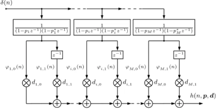
The transfer function of the PF in (8) can be rearranged as H(¨r, z) = P/2 X i=1 d i,0(¨r) +di,1(¨r)z 1 (1 pi(¨r)z 1)(1 p⇤i(¨r)z 1) , di,0(¨r) = Re{Ri(¨r)}=|Ri(¨r)|cos(\Ri(¨r)), (12) di,1(¨r) = Re{Ri(¨r)p⇤i(¨r)}=|Ri(¨r)pi|cos( i \Ri(¨r)), and implemented as a parallel of second-order filters, shown in Fig. 2, which is linear in the parameters {di,0, di,1}, but
nonlinear in the poles {pi, p⇤i}. Each second-order section
(n) 1 (1 p1z 1)(1 p⇤1z 1) 1 (1 piz 1)(1 p⇤iz 1) 1 (1 pMz 1)(1 p⇤Mz 1) z 1 z 1 z 1 d1,0 d1,1 di,0 di,1 dM,0 dM,1 h(n,p,d) '1,0(n) '1,1(n) 'i,0(n) 'i,1(n) 'M,0(n) 'M,1(n)
Fig. 2. The PF model structure (withM=P/2). The impulse responses to
the second-order IIR filters, denoted by'i,0and'i,1fori= 1, . . . , M, are
used as basis functions in a linear-in-the-parameters model structure.
models a room resonance, with resonance frequency and band-width determined by the position of{pi, p⇤i}, within the unit circle in order to ensure stability. Particular attention should be given to repeated poles, which produce polynomial amplitude envelopes on the decaying exponentials [35], the order of which is determined by the multiplicity of the repeated pole. It should be noticed that, in the presence of repeated poles, the model structure in Fig. 2 has to be modified accordingly.
III. ORTHONORMALBASISFUNCTION MODELS Parametric models based on OBFs can be derived from an orthogonalization of PF models. The orthogonality of the basis functions, together with the linearity in the parameters, introduces some desirable properties which bring a number of advantages in terms of efficiency and numerical stability in the modeling of RIRs. In this section, OBF models are also described as a generalization of other parametric models. Furthermore, their properties are described along with their application in the approximation of a target RIR.
A. Construction of OBF models
OBF models are derived with a Gram-Schmidt orthonorma-lization procedure applied to one- and two-pole filters [13]– [15]. Starting from a normalized first-order IIR filter with pole p1 and transfer function
1(z, p1) = A1 1 p1z 1 , (13) whereA1 = p
1 |p1|2 is a normalization factor, a
second-order filter with poles[p1, p2]and transfer function orthogonal
to (13) can be obtained as 2(z,[p1, p2]T) = A2(z 1 p⇤ 1) (1 p1z 1)(1 p2z 1) , (14) withA2=p1 |p2|2 and with * indicating complex
conju-gation. The orthogonality of 1and 2is provided by the zero
inz=1/p⇤
1and can be investigated via the inner product on the
Hardy space on the unit circleH2(T)(withT,{z:|z|= 1})
as (see [15]) h 1, 2i= 1 2⇡j I T 1(z) ⇤ 2(z) dz z = 0. (15)
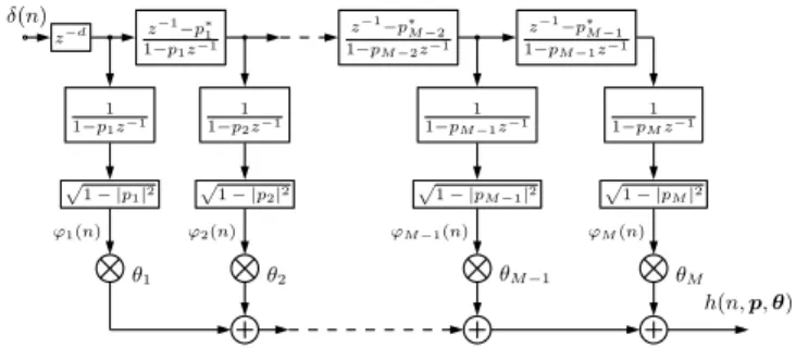
(n) z d z 1 p⇤ 1 1 p1z 1 z 1 p⇤ M 2 1 pM 2z 1 z 1 p⇤ M 1 1 pM 1z 1 1 1 p1z 1 1 p12z 1 1 pM11z 1 1 pM1z 1 p 1 |p1|2 p 1 |p2|2 p 1 |pM 1|2 p 1 |pM|2 '1(n) '2(n) 'M 1(n) 'M(n) ✓1 ✓2 ✓M 1 ✓M h(n,p,✓)
Fig. 3. The Takenaka-Malmquist OBF model structure forMreal poles.
The transfer function in (14) can be seen as the product of a normalized first-order IIR filter defined byp2and a first-order
all-pass filter defined by p1. By repeating the procedure for a
set of poles pi = {p1, . . . , pi}, the ith transfer function will consist of a normalized first-order IIR filter defined bypiand a sequence of first-order all-pass filters defined by the pole set pi 1={p1, . . . , pi 1}, i(z,pi) = p 1 |pi|2 1 piz 1 !i 1 Y l=1 ✓z 1 p⇤ l 1 plz 1 ◆ , (16)
which is also known as the Takenaka-Malmquist function [13]. The corresponding model structure is shown in Fig. 3, where the model output h(n,p,✓) is a linear combination of the
responses of the basis functions, weighted by the linear parameters✓i.
An OBF model based on the functions in (16) can be seen as a generalization of other well-known models. If all the poles are identical and real, the Laguerre model [37] is obtained, which is in turn a normalized version of a so-called warped FIR filter model [26], with the value of the warping parameter the repeated real pole. If the pole is placed in the origin, then the Laguerre filter simplifies to an AZ model.
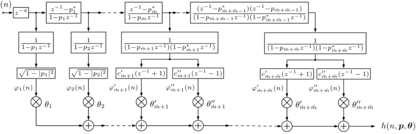
When the pole set pi contains complex poles, the basis functions in (16) are generally complex-valued and are thus not useful for the identification of real systems. As for PF models, two real-valued basis functions can be obtained by combining pairs of complex-conjugate poles, and by orthogonalizing each pair of basis functions with respect to each other (plus a normalization factor). Different realizations of an OBF model can be obtained for particular choices of these normalization factors, as explained in [15]. A combination of a Takanaka-Malmquist model and the so-called Kautz model can be used, as suggested in [20], modeling real and complex poles, respectively. This model structure, henceforth called mixed-Kautz model, is shown in Fig. 4 form˙ real poles andm¨ pairs
of complex-conjugate poles. The basis functions of a mixed-Kautz model are defined for a real pole pi as
i(z,pi) = ✓ A i 1 piz 1 ◆iY1 l=1 ✓z 1 p⇤ l 1 plz 1 ◆ , (17)
or for a complex-conjugate pole pair{pi 1, pi}={pi, p⇤
i}as 0 i(z,pi) = c0 i(z 1+ 1) (1 piz 1)(1 p⇤iz 1) iY2 l=1 (z 1 p⇤ l) (1 plz 1) , 00 i(z,pi) = c00 i(z 1 1) (1 piz 1)(1 p⇤iz 1) iY2 l=1 (z 1 p⇤ l) (1 plz 1). (18)
with Ai = p1 |pi|2, and normalization factors c0i =
|1 pi|Ai/
p
2 and c00
i = |1 +pi|Ai/
p
2. Notice that the
pair of basis functions in (18) are built as a product of a sequence ofi 2first-order all-pass filters given by the poles
inpi 2, a second-order all-pole filter defined by{pi, p⇤i}and a normalization term, so that the model structure for complex-conjugate poles is given by a parallel of orthonormalized second-order IIR filters. However, real poles may not be of much interest in the approximation of measured RTFs; even though positive real poles would be useful for modeling the cavity mode of a room response, a measured RTF has a band-pass characteristic, with a cut-off at low frequencies determined by the response of the high-pass filter of the loudspeaker, and a cut-off at high frequencies given by the low-pass behavior of the loudspeaker or the anti-aliasing filter. For this reason, only complex-conjugate poles can be considered, thus resulting in the use of a Kautz model.
B. Properties of OBF models
The orthogonality of the basis functions provides some desirable properties. First, the OBFs form a complete set in H2(T), under the assumption thatP1i=0(1 |pi|) =1[15]. Thus, by decomposing a target RIR in terms of an orthogonal expansion, the approximation error can be made arbitrarily small by choosing a large enough number of poles.
Second, orthogonality provides flexibility, which results from the fact that poles can be arbitrarily positioned inside the unit circle (for the sake of stability), and that frequency resolution can be allocated unevenly in different regions of the spectrum without numerical conditioning problems, regardless of the model order. This is not the case, for example, for PZ models, where problems of ill-conditioning and instability can arise for high model orders.
Third, OBF models are linear in the parameters✓i, which means that linear regression can be applied in order to estimate their optimal values. Moreover, due to the orthogonality of the basis functions, it is not necessary to carry out a matrix inversion, which is often a source of numerical problems. Another consequence of orthogonality is the fact that the parameters ✓i for each IIR filter are independent from the ones for others filters in the structure, so that a model of lower order can be obtained from a model of higher order only by truncation, and similarly additional poles can be included without recomputing the values of the✓i’s corresponding to the poles already used. An additional advantage of OBF models over PF models is that the same pole can be included more than once (e.g. to model modes with a double decay) without the need to modify the structure. These properties are exploited in the scalable algorithm described in Section IV.
(n) z d z 1 p⇤1 1 p1z 1 z 1 p⇤m˙ 1 pmz˙ 1 (z 1 p⇤ ˙ m+ ¨m 1)(z 1 pm˙+ ¨m 1) (1 pm˙+ ¨m 1z 1)(1 p⇤m˙+ ¨m 1z 1) 1 1 p1z 1 1 1 p2z 1 1 (1 pm˙+1z 1)(1 p⇤m˙+1z 1) 1 (1 pm˙+ ¨mz 1)(1 p⇤m˙+ ¨mz 1) p 1 |p1|2 p 1 |p2|2 c0m˙+1(z 1+ 1) c00m˙+1(z 1 1) c0m˙+ ¨m(z 1+ 1) c00m˙+ ¨m(z 1 1) '1(n) '2(n) 'm0˙+1(n) '00m˙+1(n) '0m˙+ ¨m(n) '00m˙+ ¨m(n) ✓1 ✓2 ✓0m˙+1 ✓m00˙+1 ✓0m˙+ ¨m ✓m00˙+ ¨m h(n,p,✓)
Fig. 4. The mixed-Kautz model structure form˙ real poles andm¨ pairs of complex-conjugate poles. For convenience, the basis functions corresponding to real poles defined in (17) are followed by the basis functions corresponding to complex-conjugate pole pairs defined in (18).
C. Approximation of a RIR with an OBF model
The approximation of a target RIR h(n) using an OBF
model consists in estimating the parameters in the pole set p = {pi} and in the set of parameters ✓ = {✓i}, with i= 1, . . . , M (cfr. Fig. 4 whereM = ˙m+ 2 ¨m), that minimize the distance between a target RIRh(n)and the model response h(n,p,✓) for n = 1, . . . , N. For a fixed set of poles p, the problem of estimating ✓ is linear and can be solved in closed form. The responseh(n,p,✓)of an OBF model for an impulse input signal (n) is the linear combination of the responses
'i(n,pi)of the M basis functions i(z,pi) (see e.g. Fig. 3 or Fig. 4), h(n,p,✓) = M X i=1 ✓i i(z,pi) (n) = M X i=1 ✓i'i(n,pi) ='(n,p)T✓, (19)
where'(n,p)is a vector containing the responses'i(n,pi)at timen. By stacking all the vectors'(n,p)for n= 1, . . . , N in a matrix (p) of size N ⇥M, the optimal values for ✓ for a given input-output set{ ,h}={ (n), h(n)}N
n=1can be
estimated in LS sense as
ˆ
✓= (p)Th. (20)
Note that the LS estimation does not require any matrix inversion, given that the orthonormality of the basis functions implies (p)T (p) =I
M. It can be seen from (20) that the optimal estimate for ✓ corresponds to the correlation of the basis functions in (p)with the target RIR vectorh, so that
ˆ
✓ gives the degree of similarity between each basis function and the target RIR.
The problem of estimating the optimal pole set pˆcan be
then regarded as finding the poles that generate basis functions that are maximally correlated with the target RIR, so that the approximation error between the model response and the target RIR is minimized. However, no closed-form solution to the pole estimation problem is available. The state-of-the-art approach for the multiple-poles case is the BU method
[19]–[23], an iterative nonlinear method based on FIR-to-IIR filter conversion [24]. Frequency prewarping of the target response has been proposed for audio applications in order to match a particular frequency-scale mapping, such as the Bark scale [38]. The BU method exploits the orthogonality of OBF models and provides accurate estimates for the pole parameters. However, the model order has to be predetermined, and stability problems can arise from numerical issues at high model orders.
IV. THEOBF-MPALGORITHM
The problem of sparse linear approximation of a signal con-sists in finding a compact representation by a combination of functions taken from an overcomplete basis. These functions are usually called predictors or atoms, which altogether form a basis, sometimes called dictionary. The most popular methods for sparse approximation can be divided in two main categories [39]. In the first one, convex optimization techniques are used to minimize a functional, such as the `1 norm in the Least
Absolute Shrinkage and Selection Operator (LASSO) [40]. The second category includes iterative greedy algorithms, such as Orthogonal Matching Pursuit (OMP) [41]–[43].
Our approach aims to find a sparse approximation of a target RIR as a linear combination of a finite number of OBFs. A RIR cannot be considered a sparse time-frequency signal itself, with a certain degree of sparsity only in the modal region. By first modeling dominant low-frequency modes and the spectral envelope at higher frequencies, the proposed algorithm is able to provide a sparse approximation of a RIR using a finite-order OBF model. In this section, an OMP-based greedy algorithm, which is termed here OBF-MP [29], is used to iteratively select poles from a large set of candidate poles distributed over the unit disc, thus bypassing the inherent nonlinear problem. At each iteration of the OMP algorithm, the predictor that has the highest correlation with the current residual response is selected. The problem in the OBF-MP algorithm, given that OBFs are defined by previous poles in the structure, consists in defining a dictionary of candidate predictors, where the dicti-onary has to be updated at each iteration using the predictor selected at the previous iteration. The advantage of OBF-MP over the conventional OMP algorithm is that the orthogonal
pg Build k(pg) A k 1 pA k 1 Compute correlations ↵i h s= arg maxi|↵i|
Update predicted component
ˆ xk='s↵s ↵s 's(ps) Update basis A k, nA
Update pole set pA k = [pAk 1ps] Update approximation ˆ hk=ˆhk 1+xˆk ˆ h0= 0 ˆ hk A k pA k whilenA< Mdo
Fig. 5. The OBF-MP algorithm block diagram. Inbound dashed lines represent initial conditions and inputs, while outbound dashed lines represent outputs. projection of the current residual response onto the set of predictors selected at the previous iterations is not necessary. The predictors, in fact, are already orthogonal to each other by construction. This ensures that the algorithm does not contain any matrix inversion, thus avoiding ill-conditioning problems. Moreover, since the candidate predictors are orthogonal to the predictors selected at previous iterations, computing the correlation with the current residual response is equivalent to computing the correlation with the target RIR.
Another consequence of orthogonality is the scalability of the algorithm, from which it follows that the number of parameters of the final model structure does not have to be defined in advance. A pole and the related linear coefficient are estimated at each iteration, independently of poles selected at previous iterations. It follows that additional poles can be estimated just by running extra iterations of the algorithm, wit-hout any problem of instability or numerical ill-conditioning. This scalability property of the algorithm is also a consequence of the fact that, similarly to what was discussed at the end of Section II for PF models, also OBF models can be regarded as a way of approximating a RTF. It has been already mentioned that, for the same set of non-repeated poles, the basis functions of a PF model and the ones of an OBF model span the same approximation space, so that it is possible to convert the values of the linear parameters from one model form to the other by simply a linear transformation [5].
Following the above interpretation, the idea of the OBF-MP algorithm is to iteratively compute a sparse approximation ˆh
of a target RIRhof lengthN samples as a linear combination of length-NOBFs, analogously to the definition of a RIR as a summation of exponentially decaying functions, independent one from each other. The OBFs are selected from a dictionary k of candidate predictors 'i (i = 1, . . . , D) and included in the basis A
k. At each iterationk,D candidate predictors
'i, orthogonal to the predictors in the current basis Ak 1
constructed with the current set of active poles pAk, are built from Gpoles placed arbitrarily in a gridpg inside the upper half of the unit disc. The matrix k has dimensions N⇥D, with D = ˙m+ 2 ¨m where m˙ andm¨ denote respectively the
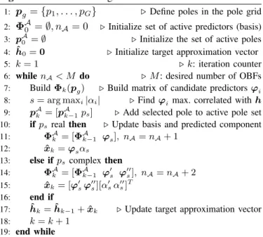
Algorithm 1 OBF-MP algorithm
1: pg={p1, . . . , pG} . Define poles in the pole grid
2: A0 =;, nA= 0 .Initialize set of active predictors (basis)
3: pA
0 =; .Initialize the set of active poles
4: h0ˆ =0 .Initialize target approximation vector
5: k= 1 .k: iteration counter
6: whilenA< M do .M: desired number of OBFs
7: Build k(pg) .Build matrix of candidate predictors'i
8: s= arg maxi|↵i| .Find'imax. correlated withh
9: pA
k = [pAk 1ps] .Add selected pole to active pole set
10: ifps realthen .Update basis and predicted component
11: A
k = [ Ak 1 's], nA=nA+ 1
12: xˆk='s↵s
13: else ifps complexthen
14: A
k = [ Ak 1 '0s '00s], nA=nA+ 2
15: xˆk= ['0s's00][↵0s↵00s]T
16: end if
17: ˆhk=ˆhk 1+xˆk .Update target approximation vector
18: k=k+ 1
19: end while
number of real poles and complex poles in the gridpg, so that G= ˙m+ ¨m.
The OBF-MP algorithm is described in detail below, and a graphical representation is depicted in Fig. 5. First, a grid of Gcandidate poles pg is defined, similarly to [28]–[30], with poles distributed according to a desired frequency resolution or prior knowledge about the system. In [28]–[30], the angle and the radius of the poles were distributed either uniformly or logarithmically on the unit disc, with the latter option intended to increase the resolution at low frequencies. Here, a different pole grid is used, depicted in Fig. 6, henceforth referred to as Bark-exp grid; the radius ⇢i of the poles decreases exponentially at the increase of the angle i, as suggested in [23], according to⇢i =%
i
⇡, with%the value of the radius defined at the Nyquist frequency. Regarding the values for
%, it is suggested here to set the number of radii for each angle and distribute them logarithmically in order to increase density toward the unit circle. Differently from [23], in which the angles follow a logarithmic scale, the Bark frequency scale [38] was chosen. The Bark scale further increases the resolution at low frequency, providing an effect similar to the prewarping of the RIR used in the wBU method. In this way, a higher density of poles close to the unit circle is achieved at low frequencies, allowing a more accurate approximation of energetic and narrow-bandwidth resonances, while at higher frequencies poles sparser in frequency and more distant from the unit circle provide a coarser approximation.
At the first iteration, the current basis A
0 and the set of
active poles pA
0 are empty (with the number of predictors in
the basisnA= 0). Also the target approximation vectorˆh0, is
initially set to zero. At each iterationk, the matrix of candidate predictors k(pg) is updated according to the mixed-Kautz structure in Fig. 4. The matrix khas always dimensionN⇥ D (since an OBF model admits repeated poles, a pole that is selected by the algorithm is not removed from the pole gridpg) and its columns are the OBFs built from the poles inpg with
1 0.5 0 0.5 1 1 0.5 0 0.5 1 Real part Imaginary part
Fig. 6. The Bark-exp pole grid for the OBF-MP algorithm (here with
5 radii and 400 angles and upper angle limited to 0.8⇡).
'0i '00i ↵i h ↵0i ↵00i
Fig. 7. Graphical interpretation of the correlation between the target RIR vectorhand the predictors of a pair of complex-conjugate poles{pi, p⇤
i}.
transfer functions as in (17) and in (18), thus orthonormal to the predictors in the current basis A
k 1 built from the poles
in the current active pole set pAk 1. The predictor(s) in k that has the largest absolute correlation↵iwith the target RIR vector h is selected and added to the basis Ak, while the corresponding pole is included in the set of active poles pAk. The correlation for real and complex poles is computed in two different ways. For real poles, the correlation is the projection ofhonto the predictor'i(↵i='Tih). For a pair of complex-conjugate poles {pi, p⇤
i}the correlation is the projection ofh on the plane defined by predictors '0
i and '00i(see Fig. 7), which are mutually orthogonal, and is given by
↵i= q ↵0 i 2 +↵00 i 2 = q ('0 i T h)2+ ('00 i T h)2. (21)
The kth predicted component xˆ
k is obtained from the last added predictor(s) using the maximum correlation ↵s as re-gression coefficient (with s= arg maxi|↵i|), byxˆk='s↵s, if the selected pole is real, or by xˆk = ['0s's00][↵0s↵00s]T, otherwise. The current target RIR approximation vectorˆhk is
obtained by adding the predicted componentxˆkto the previous target RIR approximation vector hˆk 1. As a consequence
of its scalability property, the algorithm can terminate when the desired number M of predictors in the basis is reached, or alternatively when the approximation error falls below a desired value.
A. Algorithmic complexity analysis
Here the asymptotic computational complexity of the OBF-MP algorithm is analyzed, assuming for simplicity that only complex poles are included in the pole grid. With reference to Algorithm 1, there are two operations that determine the asymptotic behavior of the algorithm. Building the matrix k of candidate predictors (step 7) at each iteration is the
most demanding operation, which involves the generation of D predictors of length N, which sums up to a complexity of O(3N D) multiplications (cfr. the expressions in (18) and Figure 4). The second operation to consider is the computation of the correlation coefficients (step 8), which is a multipli-cation of the matrix k with the vector h of length N, which results in O(N D) multiplications. The computational
complexity associated to vector updates and other operations is negligible. The overall complexity of the OBF-MP algorithm after k=M/2 iterations, is O(2M N D)multiplications, i.e.
linearly proportional to the three variables considered. In other words, the computational complexity increases linearly with the length of the impulse response, the number of candidate poles, and the number of iterations. This is comparable with the complexity of the BU method, whose most demanding operation is represented by the solution to a set of overde-termined linear equations, which implies a QR factorization of a largeN⇥M rectangular matrix (complexityO(N M2)),
followed by a back-substitution of aM⇥M triangular matrix (complexityO(M2)) [44]. This is performed forI iterations,
with the overall computational complexity of the BU method summing up toO(IN M2), which is quadratic with respect to
the number of estimated polesM.
V. MODEL ANDFILTERCOMPLEXITY
In this section, the complexity of the parametric models presented in the previous sections will be analyzed from two different perspectives. First, the model complexity (or repre-sentation complexity)Cm is considered, which is the number of parameters that is necessary to represent the system under study. Second, thefilter complexity(orsimulation complexity) Cfis considered as the number of operations that are required to obtain the filter output signal for a given input signal when the parameter values are available. While a measure often used in the literature is the model order, it is believed that the two concepts just proposed are less prone to misinterpretation and thus preferable for the comparison of different parametric models in terms of complexity. For simplicity, OBF models and PF models having complex-conjugate pole pairs only are considered.
1) Model complexity: The calculation of the model com-plexity Cm is straightforward for AZ and PZ models. By referring to (5) and (6), the number of parameters for AZ models corresponds to the number of numerator coefficients (Cm = Q + 1), while for PZ models it is the sum of denominator and numerator coefficients (Cm=P+Q+1). For PF models, ifP/2 is the number of complex-conjugate poles pairs, the number of parameters required isCm = 2P, since each second-order section can be represented with one polepi (which is a complex number defined by two parameters, while p⇤
i is given by complex conjugation) and two linear parameters (denoted bydi,0 anddi,1 in (12) and in Fig. 2). The same is
obtained for OBF models, in which the all-pass filters and the normalization factors can be computed from the knowledge of the poles (see e.g. Fig. 4). The model complexity Cm is summarized in the left column of Table I.
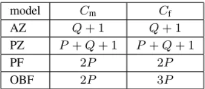
TABLE I
MODEL AND FILTER COMPLEXITY
model Cm Cf
AZ Q+ 1 Q+ 1
PZ P+Q+ 1 P+Q+ 1
PF 2P 2P
OBF 2P 3P
2) Filter complexity: The filter complexityCf is calculated here as the number of multiplications required to compute the filter output for a given input signal. For AZ and PZ models, one multiplication is required for each coefficient, so that Cf=Cm. This is true also for PF models, in which four multiplications are required for each second-order section, two for the second-order IIR filter and two for the linear parameters (see Fig. 2). In case of repeated poles, the structure has to be modified, but the number of multiplications remains the same [35]. For OBF models, the normalization coefficients c0i and c00i can be combined together with the related linear parameters ✓0i and ✓i00, so that the only difference between OBF models and PF models in terms of filter complexity is determined by the orthogonalization. By including the second-order all-pass filters in the structure, two more multiplications per section have to be included (assuming that the input of the all-pass filter is the output of the previous second-order IIR filter), summing up to six per section, so that the filter complexity for P/2 pairs {pi, p⇤i} is Cf = 3P. The filter complexity Cf is summarized in the right column of Table I. Notice that an OBF model is more complex than a PF model. However, these two models span the same approximation space for the same set of poles, thus leading exactly to the same filter response when the optimal linear coefficients are computed using the `2 norm in LS design. It would be then
possible to convert an OBF model into a PF model with lower filter complexity, as was also suggested in [4].
VI. SIMULATION RESULTS
The modeling performance of the OBF-MP algorithm des-cribed in Section IV was tested onR= 41RIRs measured for
several source-receiver positions in three different rooms with different reverberation times. The RIRs were taken from three publicly available databases, namely MARDY [45], SMARD [46], and MIRD [47]. A fourth database of 24 low-frequency RIRs, called SUBRIR [48], was used separately to evaluate the modeling performance of the algorithm in the modal frequency region, as will be discussed later in this section. Their speci-fications, such as the room volume V, the surface areaS, the reverberation timeT, the Schroeder frequencyfSchcomputed as in (4), and the mixing time tm, are listed in Table II. According to [49], the most accurate estimate of the mixing timetm, i.e. the time instant at which the diffuse reverberation tail begins, is given by a formula related to the concept of mean free path length, given by tm = 20V /S+ 12 (in ms). Notice that the MIRD database includes RIRs measured in a room where the reverberation time is controlled by means of movable acoustic panels, resulting in 3 different values of
TABLE II DATABASE SPECIFICATIONS database V (m3) S(m2) tm(ms) T(s) fSch(Hz) RIRs SMARD 170.4 207.3 28.4 0.15 59 8 MARDY 208.8 255.6 28.0 0.45 93 9 0.16 86 8 MIRD 86.4 129.6 25.3 0.36 129 8 0.61 168 8 SUBRIR 62.3 102.1 24.2 0.5-1.5 >180 24
T in Table II. All target RIRs are sampled at fs = 48 kHz and truncated toN = 6000samples. This corresponds to the shortest ‘useful duration’, defined as the time instant where the SNR of the measured RIR is10 dB[50]. In order to compute the SNR value, the decay curve and the noise floor level were estimated with the method by Lundeby et al. [51]. Since the modeling of the delay of the RIR is not part of the scope of this paper, the direct path component was considered as the starting point of the RIR. However, a simple delay could be easily included in the model structure of the OBF model by setting the parameter din Fig. 4.
In the simulations presented in this section, an approximated response ˆh(r), with r = 1, . . . , R, was computed for each
target RIR h(r) using the OBF-MP algorithm. OBF models obtained with OBF-MP were compared to AZ and PZ models and to OBF models obtained with the warped BU (wBU) met-hod suggested in [22], henceforth called OBF-wBU models. The measure used to compare the performance of different models with the same model complexityCm is the normalized mean-square error (NMSE), averaged over allR RIRs, which in the time domain is given by
hNMSE(dB) = 10 log10 1 R R X r=1 khr ˆhrk22 khrk22 , (22) while the average frequency response NMSE is defined as
HNMSE(dB) = 10 log10 1 R R X r=1 kHr Hˆrk22 kHrk22 , (23)
with Hr and Hˆr the Discrete Fourier Transform (DFT) of hr and hˆr, respectively. The NMSE was computed on the complete time response (hfull
NMSE), and on the early (h early NMSE) and
late (hlate
NMSE) responses separately. The time instant separating
the two parts was set to 25ms, corresponding to the shortest mixing timetmfor the three rooms considered (see Table II). Also the NMSE in the frequency response was analyzed for the frequency range between0 Hzand20 kHz(Hfull
NMSE), as well as
at low/mid frequencies between 0 and4 kHz (Hlow/mid NMSE ), and
at high frequencies between 4 kHz and 20 kHz (Hhigh NMSE), in
order to show the differences in performance of the models in different frequency ranges. Although the Schroeder frequency in (4) would have been a more natural choice for separating the frequency range, its value in the databases considered was found to be below or just above the lower cut-off frequency of the loudspeaker used for the measurements. The upper limit of
20 kHz was chosen to avoid considering the frequency range
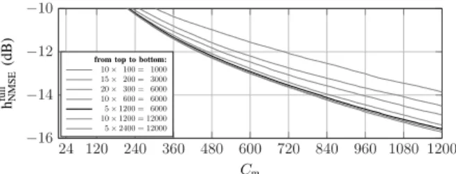
24 120 240 360 480 600 720 840 960 1080 1200 16 14 12 10 Cm h full NMSE
(dB) from top to bottom: 10⇥100 = 1000 15⇥200 = 3000 20⇥300 = 6000 10⇥600 = 6000 5⇥1200 = 6000 10⇥1200 = 12000 5⇥2400 = 12000
Fig. 8. The average time-domain NMSE in (22) for different pole allocations and densities of a Bark-exp grid. The darker line indicates the grid chosen for the simulations.
The Bark-exp grid used in these simulations counts G = 6000 poles with 5 different radii distributed logarithmically with values %at Nyquist from 0.5 to 0.99, and 1200 different angles placed from 48 Hz to19.2 kHzaccording to the Bark frequency scale [38] with Bark-warping factor w = 0.766.
The limits on the angle were chosen to avoid approximating the response below the cut-off frequency of the loudspeakers and above the cut-off frequency of the anti-aliasing filter. As a result, the grid contains only complex poles. The reason of such an uneven allocation of the number of radii and angles is due to the frequency resolution that is required to approximate low-frequency resonances and to the observation that increasing the resolution in the angle is more important than in the radius. Using 1200 angles provides a constant resolution of 2.5 Hz below 500 Hz; this seems to be already a sufficient resolution, as confirmed by the results depicted in Fig. 8, showing the average full-response time-domain NMSE over a selection of 10 RIRs, computed for different allocations of radii and angles of poles in the Bark-exp grid. It should be noted in the figure that doubling the number of poles in the grid from 6000 to 12000 does not provide a significant increase in the accuracy.
The wBU method, also using Bark-warping factor w = 0.766, was slightly modified in order to avoid numerical instabilities. Although it has been proved in [24] that the BU method provides a stable IIR filter by conversion of an FIR filter, we observed cases where the solution with the minimum conversion error contains poles outside the unit circle. In the same paper, instabilities were noticed in those cases where the FIR filter was maximum-phase. However, in those cases, the conversion error was supposed to be high, so that it was always possible to find a stable solution with low conversion error. In [22], numerical limitations were observed in the wBU method and in the computation of the roots of the poles for a number of parameters Cm above 300. Since higher values of Cm were considered in our simulations, the wBU method was modified by choosing the first stable solution with minimum conversion error. The number of iterations was set to 100. For PZ models, the STMCB method [25] with P = Q+ 1
parameters has been used, with the initial estimate obtained with Prony’s method [52]. In order to reduce the number of unstable solutions, only three iterations were executed.
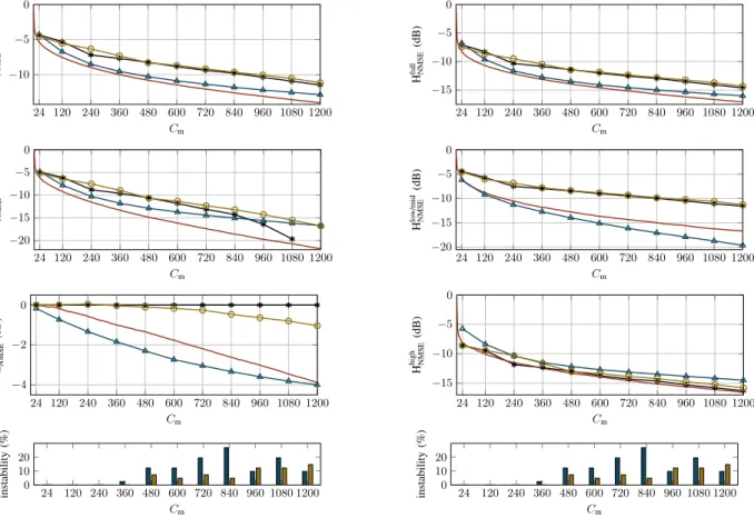
Fig. 9 presents simulation results comparing the perfor-mance of the different models for varying model complexity Cm. The MATLAB code for generating the results presented
in this section is available online1. The NMSE produced by OBF models obtained with OBF-MP was computed at each iteration, while for other models the NMSE was computed only for given values of Cm. In the bottom row of the figure, the occurrences of unstable solutions given by the wBU method and the STMCB method are reported. For the wBU method, the first stable solution was used, as described above, while for PZ models, unstable solutions were removed from the calculation of the average NMSE. It is clear that both methods suffer from instability due to ill-conditioning above certain values of Cm.
In the left column of Fig. 9, results for the NMSE in the time domain defined in (22) are given for the complete response, for the early reflections and for the late reverberation. The plot on top shows that OBF models provide in general a better approximation of the target RIR overN samples, with OBF-MP outperforming AZ models even in the approximation of the early response (middle plot), except when AZ models achieve perfect modeling (at Cm = 1200,hearlyNMSE(dB) = 1 for AZ models). Focusing on OBF models, OBF-MP shows an overall improvement over OBF-wBU, with the former having a better performance in the early part of the response and the latter performing better in the late part (bottom plot).
The plots in the right column of Fig. 9 show results in the frequency domain. Results in the frequency range between0
and4 kHzshow a clear improvement in the approximation of
the low/mid frequencies given by OBF models, with OBF-MP and OBF-wBU having a similar performance for smallCm, but with an increased accuracy for increasingCmprovided by the wBU method. This does not imply a degraded performance in the higher part of the spectrum, where OBF models give an error comparable to the error of AZ and PZ models, with OBF-MP providing an improvement over OBF-wBU and the other models, as can be seen in the plot at the bottom (this improvement is less visible than above, given the larger frequency range considered).
In general, differences in the performance of OBF-MP and OBF-wBU are a result of the inherent discretization of the MP algorithm; its limited resolution prevents the OBF-MP algorithm from perfectly matching the frequency and bandwidth of some magnitude peaks. As a consequence, these peaks are approximated using poles with a slightly shorter radius, which corresponds to a larger bandwidth and a shorter decay of the time response; which is the reason why OBF-wBU shows better performances at low frequencies and in the late response. On the other hand, OBF-MP has a higher resolution at higher frequencies and, as a result, a better performance in that frequency region and in the approximation of the early response.
These results can be visualized on the approximated fre-quency magnitude responses of the example in Fig. 10, showing the more accurate approximation of low-frequency resonances provided by OBF models with a Bark-scale reso-lution compared to AZ and PZ models, with the OBF model obtained with wBU performing better than the OBF-MP, for the reason explained above. However, a large error is
24 120 240 360 480 600 720 840 960 1080 1200 10 5 0 Cm h full NMSE (dB) 24 120 240 360 480 600 720 840 960 1080 1200 15 10 5 0 Cm H full NMSE (dB) 24 120 240 360 480 600 720 840 960 1080 1200 20 15 10 5 0 Cm h early NMSE (dB) 24 120 240 360 480 600 720 840 960 1080 1200 20 15 10 5 0 Cm H lo w/mid NMSE (dB) 24 120 240 360 480 600 720 840 960 1080 1200 4 2 0 Cm h late NMSE (dB) 24 120 240 360 480 600 720 840 960 1080 1200 15 10 5 0 Cm H high NMSE (dB) 24 120 240 360 480 600 720 840 960 1080 1200 0 10 20 Cm instability (%) 24 120 240 360 480 600 720 840 960 1080 1200 0 10 20 Cm instability (%)
Fig. 9. The average NMSE vs. the model complexityCm. (left) The average time-domain NMSE in (22) for the entire response (top) and for the early (middle) and late response (bottom). (right) The average frequency-domain NMSE in (23) for the entire frequency range (top)
and for the frequency regions [0,4] kHz (middle) and [4,20] kHz (bottom). AZ models (⇤), PZ models ( ), OBF models obtained with
OBF-wBU (MMM) and with OBF-MP ( ). At the bottom, occurrences of unstable solutions for OBF models obtained with OBF-wBU (left
bars) and PZ models (right bars) are reported (same plot on both columns).
introduced by OBF-wBU at high frequencies, while OBF-MP is able to better approximate the envelope of the magnitude response. Looking at the selected pole sets for the different models, some differences can be observed: for PZ models, the poles are evenly distributed in the entire Nyquist interval, while for OBF models, the poles are mostly concentrated in the low frequencies (and closer to the unit circle), with a larger concentration in the very low frequencies for OBF-wBU models. It should be noted that, while the OBF-wBU method allows to control the frequency resolution only by means of the warping parameter, the pole grid of the OBF-MP algorithm offers more flexibility in the selection of the candidate poles and the possibility of incorporating prior knowledge about the characteristics of the room.
As discussed in Section V, another important aspect to consider when comparing different parametric models is their filter complexity Cf. While the filter complexity Cf for AZ and PZ models equals the model complexityCm, OBF models require extra computations (cf. Table I). As an illustrative example, Fig. 11 shows the error of the different models as a function of the filter complexity Cf, and should be compared to the top-left plot of Fig. 9. The corresponding model complexityCmfor OBF models is reported on the axis underneath. It can be seen that using OBF models gives a
smaller average NMSE compared to AZ and PZ models also in terms of filter complexity. Given the equivalence in terms of filter response between OBF models and PF models, the number of multiplications for OBF models can be reduced by using a PF implementation (in which caseCf equalsCm).
In order to perform the same kind of analysis in the modal region, similar simulations were run on the SUBRIR database [48], [53]. The SUBRIR database is a collection of RIRs measured at low frequency using a subwoofer as a source. Here, a subset of R = 24 RIRs measured with a
Genelec 7050B subwoofer (with frequency range 25-120 Hz) and a B&K 4133 (1/2”) microphone was used. The RIRs were downsampled to fs = 800 Hz and truncated to 1.5 s
(corre-sponding to the maximum reverberation time, as reported in Table II and in [48]).
The OBF-MP grid used is this case has 600 angles uni-formly placed from 0 to⇡ (the Bark scale below 500 Hzhas
uniform resolution) and 10 radii logarithmically distributed from 0.75 to 0.999, while the BU method is applied without prewarping. The top plot of Fig. 12 shows the error of the different models as a function of the filter complexity Cf, similarly to Fig. 11. As in the previous examples, although OBF-MP models and OBF-BU models perform similarly, the BU method leads to numerical conditioning problems and to
100 1000 10000 20 10 0 10 All-Zero Magnitude (dB) 100 1000 10000 20 10 0 10 Pole-Zero Magnitude (dB) 1 0.5 0 0.5 1 0 0.5 1 100 1000 10000 20 10 0 10 OBF-wBU Magnitude (dB) 1 0.5 0 0.5 1 0 0.5 1 100 1000 10000 20 10 0 10 OBF-MP (Bark-exp) Log-scaled Frequency (Hz) Magnitude (dB) 1 0.5 0 0.5 1 0 0.5 1
Fig. 10. Approximated magnitude responses for (from top to bottom) an AZ model, a PZ model, OBF models with the wBU method and
with the proposed method using a 5⇥1200 Bark-exp pole grid,
together with the corresponding selected pole set (Cm = 300). The
target response (from MARDY) is shown in gray.
24 120 240 360 480 600 720 COBFm 24 120 240 360 480 600 720 840 960 1080 1200 10 5 0 Cf=CmAZ,PZ h full NMSE (dB)
Fig. 11. The average time-domain NMSE in (22) for the entire
response for different values of filter complexity Cf. AZ (⇤), PZ
( ), OBF-wBU (MMM) and OBF-MP ( ) models. The filter complexity
corresponds to Cmfor AZ and PZ models, while the corresponding
values ofCmfor OBF models are shown in the additional axis.
unstable solutions for values of the model complexity as low as Cm = 240. PZ models were not considered here, as the STMCB algorithm provided unstable solutions almost in every situation. In this case, the improvement obtained with OBF models with respect to AZ models is more accentuated than in the previous examples. The reason for this is that in the modal region the number of room resonances is low and the models
24 120 240 360 480 600 720 840 50 25 0 h full NMSE (dB) 24 120 240 360 480 COBFm 24 120 240 360 480 600 720 840 50 25 0 Cf=CmAZ H { 20-130 Hz } NMSE (dB)
Fig. 12. SUBRIR database. (top) The average time-domain NMSE in
(22) for the entire response w.r.t. the filter complexityCf. (bottom)
The average frequency-domain NMSE in (23) between 20 Hz and
130 Hz w.r.t. the filter complexity Cf. AZ (⇤), OBF-BU (MMM) and OBF-MP ( ) models. 1 0.5 0 0.5 1 0 0.5 1 OBF-MP 1 0.5 0 0.5 1 0 0.5 1 OBF-BU
Fig. 13. SUBRIR database. The set of 40 complex-conjugate
pole-pairs (Cm= 160) obtained with OBF-MP (left) and the BU method
(right) in the approximation of one RIR (fs= 800 Hz).
based on OBFs provide a more meaningful approximation of a RTF than AZ models, as discussed in Section III.
The comparison of the performance of MP and OBF-BU in the frequency region of the loudspeaker, instead, pre-sents significant differences (bottom plot). Our interpretation is that the ill-conditioning problems of the BU method are worsened by the fact that the spectrum above130 Hzcontains only noise. The result is that also poles above that frequency are estimated. The poles selected by the well-conditioned OBF-MP algorithm, even though the poles in the grid are placed from 0 to ⇡, are instead well concentrated within the
range of the loudspeaker response, as shown in Fig. 13. VII. CONCLUSION ANDFUTURE WORK
The use of OBF models for obtaining a compact and accurate approximation of a target RIR has been motivated by the desirable properties derived from orthogonality, such as an improved numerical conditioning in the estimation of the numerator parameters of the transfer function for a fixed denominator. However, also OBF models are nonlinear in the parameters, so that the estimation of the poles is still a nonlinear problem. The state-of-the-art technique, the BU method, based on an FIR to IIR conversion which exploits the orthogonality property of OBF models, has some restrictions.
In this paper, the novel algorithm, termed OBF-MP, has been studied and compared to the BU method in terms of modeling performance. Simulation results for RIRs measured in different rooms showed that OBF models are able to achieve a reduction in the approximation error compared to conventional parametric models for the same model and filter complexity, provided that the estimation of the pole parameters is accurate. Although the two algorithms considered for the estimation of the poles in an OBF model seem to have similar modeling capabilities, they present many differences. While the BU method suffers from numerical conditioning problems and instability, the OBF-MP algorithm always delivers stable and well-conditioned OBF model estimates. Indeed, the OBF-MP algorithm bypasses the nonlinear problem of estimating the poles of an OBF model by defining a set of candidate stable poles and by selecting a complex-conjugate pole pair at each iteration based on the correlation between the target RIR and the basis functions built from the candidate poles. Orthogonality of the basis functions assures that this operation is numerically well-conditioned.
Moreover, while the BU-method requires the number of po-les to be determined before estimation, the OBF-MP algorithm is scalable, in the sense that a new pair of complex-conjugate poles can be estimated independently of the poles estimated at previous iterations. Scalability turned out to be related to the analogy between OBF models and the definition of the RIR as an infinite summation of exponentially decaying sinuosoids independent from each other. The OBF-MP algorithm follows this interpretation by creating an approximation of the target RIR by adding a pair of OBFs and reducing the approximation error at each iteration. Differences in the performance between OBF-MP and OBF-BU in different time and frequency regions are a consequence of the approach to the pole estimation pro-blem. While the BU method does not make any assumption on the position of the poles and controls the frequency resolution only by prewarping of the target RIR, the grid of candidate poles of the OBF-MP algorithm is an important design choice that adds a layer of flexibility. Any desired frequency resolu-tion could be obtained, motivated by prior knowledge about the acoustics of the room or by application requirements. In this paper, the Bark-exp grid was introduced to provide an accurate approximation at low frequencies, following the physical interpretation described above. However, the Bark-exp grid provides low resolution at high frequency, so that for larger model complexities, i.e. after the dominant modes and the spectral envelope have been approximated, pole grids with higher resolution at high frequencies can become more efficient. A possibility to overcome this issue could be to refine the estimation of the poles at each iteration using numerical optimization methods. This possibility and the inclusion of prior knowledge about the system in the estimation problem is left for future work.
The computational complexity of the OBF-MP algorithm is determined by the length of the target RIR sequence, the number of poles in the grid and the number of model parame-ters, and it is comparable with the algorithmic complexity of the BU method. Different approaches have been presented for reducing the complexity of the BU method and overcome its
limitations, such as subband modeling [21], polyphase design and successive segmentation in the time domain [27]. It is believed that such extensions could be applied to the OBF-MP algorithm as well. Another interesting aspect is the possibility of exploiting the concept of common acoustical poles, as considered e.g. in [11] and [54]. The OBF-MP algorithm was modified in [53] in order to estimate a common set of poles from measurements taken for different source-receiver positions inside a room. It has been shown that a significant reduction in the number of parameters necessary to model the RTF for different source-receiver positions can be achieved. A block-based version of the OBF-MP algorithm has been proposed in [55] and applied in [56] to the estimation of the poles of an adaptive IIR filter based on OBFs from input-output data of a SIMO room acoustic system. Results show that poles can be accurately estimated from white input-output data as well, offering a reduced approximation error compared to FIR filters, with the same convergence rate and complexity of the adaptation algorithm for the linear coefficients, but an improved robustness to the variability of the RTF for different source-receiver positions. Further research will focus on understanding the relation between the estimated common poles and the acoustic characteristics of the room, and on estimating the poles from nonstationary input-output data.
ACKNOWLEDGMENT
This research work was carried out at the ESAT Laboratory of KU Leuven, in the frame of (i) the FP7-PEOPLE Marie Cu-rie Initial Training Network ‘Dereverberation and Reverbera-tion of Audio, Music, and Speech (DREAMS)’, funded by the European Commission under Grant Agreement no. 316969, (ii) KU Leuven Research Council CoE PFV/10/002 (OPTEC), (iii) Research Project FWO no. G.0763.12 ‘Wireless Acoustic Sensor Networks for Extended Auditory Communication’, and (iv) was supported by a Postdoctoral Fellowship (F+/14/045) of the KU Leuven Research Fund. The scientific responsibility is assumed by the authors.
REFERENCES
[1] J. Mourjopoulos and M. A. Paraskevas, “Pole and zero modeling of room transfer functions,” J. Sound Vib., vol. 146, no. 2, pp. 281–302, 1991.
[2] G. Long, D. Shwed, and D. Falconer, “Study of a pole-zero adaptive echo canceller,”IEEE Trans. Circuits Syst., vol. 34, no. 7, pp. 765–769, 1987.
[3] A. V. Oppenheim, R. W. Schafer, and J. R. Buck,Discrete-time Signal Processing (2Nd Ed.). Upper Saddle River, NJ, USA: Prentice-Hall, Inc., 1999.
[4] B. Bank, “Perceptually motivated audio equalization using fixed-pole parallel second-order filters,” IEEE Signal Process. Lett., vol. 15, pp. 477–480, 2008.
[5] ——, “Audio equalization with fixed-pole parallel filters: An efficient alternative to complex smoothing,” inPreprints Audio Eng. Soc. Conv. 128, 2010.
[6] ——, “Computationally efficient nonlinear Chebyshev models using common-pole parallel filters with the application to loudspeaker mo-deling,” inPreprints Audio Eng. Soc. Conv. 130, 2011.
[7] B. Bank and J. O. Smith, III, “A delayed parallel filter structure with an FIR part having improved numerical properties,” inPreprints Audio Eng. Soc. Conv. 136, 2014.
[8] J. R¨am¨o, V. V¨alim¨aki, and B. Bank, “High-precision parallel graphic equalizer,”IEEE/ACM Trans. Audio, Speech, Lang. Process., vol. 22, no. 12, pp. 1894–1904, 2014.
![Fig. 1. RIR measured in the Speech Lab at KU Leuven [33].](https://thumb-us.123doks.com/thumbv2/123dok_us/9724881.2854039/3.918.470.809.87.208/fig-rir-measured-speech-lab-ku-leuven.webp)