(wileyonlinelibrary.com)DOI:10.1002/asl.787
Tuning of length-scale and observation-error for radar
data assimilation using four dimensional variational
(4D-Var) method
Yonghan Choi,1,2 Dong-Hyun Cha1* and Joowan Kim3
1School of Urban and Environmental Engineering, Ulsan National Institute of Science and Technology, Ulsan, South Korea 2Mesoscale and Microscale Meteorology Laboratory, National Center for Atmospheric Research, Boulder, CO, USA 3Department of Atmospheric Sciences, Kongju National University, Gongju, South Korea
*Correspondence to:
Prof. D.-H. Cha, School of Urban and Environmental Engineering, Ulsan National Institute of Science and Technology, 50 UNIST-gil, Ulsan 44919, South Korea. E-mail: [email protected] Received: 9 February 2017 Revised: 28 July 2017 Accepted: 17 September 2017 Abstract
The effects of tuning of length-scale and observation-error on heavy rainfall forecasts are investigated. Length scale and observation error are tuned based on observation minus background (O−B) covariances and theoretically expected cost function values, respectively. Tuned length scale and observation error are applied to radar data assimilation using the Four Dimensional Variational (4D-Var) method. Length-scale tuning leads to improved Quantitative Precipitation Forecast (QPF) skill for heavy precipitation, better analyses, and reduced errors of wind, temperature, humidity, and hydrometeor forecasts. The effects of observation-error tuning are not as significant as those of length-scale tuning, and they are limited to improvements in QPF skill. This is because tuned observation errors are close to pre-assumed values. Proper tuning of length-scale and observation-error is essential for radar data assimilation using the 4D-Var method.
Keywords: length-scale tuning; observation-error tuning; radar data assimilation; 4D– Var
1. Introduction
With the increase in resolution of numerical weather prediction models, the importance of radar data assim-ilation has been emphasized in recent years, espe-cially for forecasting high-impact weather events (Sun, 2006). Various sophisticated data assimilation methods such as variational, ensemble-based, and hybrid meth-ods have been used for assimilating radar observations. Xiao et al. (2005) examined the impact of assimilat-ing radar radial velocity on the prediction of a heavy rainfall event by implementing the observation oper-ator and the Richardson balance equation within the fifth-generation Pennsylvania State University-National Center for Atmospheric Research Mesoscale Model (MM5) Three Dimensional Variational (3D-Var) sys-tem. Wanget al.(2013a) assimilated retrieved rainwater and estimated in-cloud water vapor instead of assimilat-ing radar reflectivity directly to avoid the linearization error of the reflectivity observation operator by using the Weather Research and Forecasting (WRF) 3D-Var system. In Wanget al.(2013b), the WRF 4D-Var radar data assimilation system was introduced by develop-ing tangent-linear and adjoint of a Kessler warm-rain microphysics scheme, and by including cloud water, rainwater, and vertical velocity as new control variables. Background error covariance determines how the observation information spreads horizontally, ver-tically, and among variables. Therefore, accurate estimation and proper tuning of background error statis-tics are essential for successful data assimilation. There
have been previous studies about tuning of the length scale of background error correlation within the 3D-Var framework by using the method of Hollingsworth and Lönnberg (1986) (e.g. Lee et al., 2010; Ha and Lee, 2012). Determining the observation error covariance is one of the challenging issues in data assimilation, and only observation error variance is considered in general. Because the ratio between background and observation error variances determines relative weights given to the background and observation, a precise esti-mation of background and observation error variances is of critical importance in data assimilation. Sev-eral approaches have been tested to tune observation error variance in previous studies (e.g. Desroziers and Ivanov, 2001; Desroziers et al., 2005; Chapnik et al., 2006; Lupuet al., 2015). The objective of this study is to investigate the effects of tuning of background-error correlation length-scale and observation-error variance on forecasts of heavy rainfall cases when assimilating radar observations using the 4D-Var method.
2. Theoretical backgrounds
2.1. Length-scale tuning
Following Hollingsworth and Lönnberg (1986), the length scale of a background error correlation can be tuned using O−B values. For this, two assump-tions are necessary: (1) there is no correlation between background and observation errors and (2) observation
errors are spatially uncorrelated. In this study, thin-ning of original radar observations to 6-km mesh was adopted to minimize a potential violation of the second assumption. The process for tuning of length scale can be summarized as follows.
(1) For a specific level, calculate O−B covariances between two observation points and make a histogram of O−B covariances using the distance between the two points as a bin.
(2) Find a Gaussian function that best fits O−B covariances. B=B0exp [ − r 2 2(2s)2 ] (1) where B is O−B covariance,ris distance,B0is back-ground error variance, andsis length scale.
(3) After taking the natural logarithm of both sides of Equation (1), find the slope and intercept values for a linear relationship using the least-square regression method.
lnB=lnB0− r2
8s2 →y=intercept+slope×x (2) (4) From the slope value computed in step 3, calculate length scale,s. s= √ − 1 8·slope (3) 2.2. Observation-error tuning
From Desroziers and Ivanov (2001), expectation values of background and observation cost functions at the minimum can be given as follows.
E(Jb)= 1 2Tr(KH),E(J o) = 1 2 [ nobs−Tr(HK) ] (4) K =BHT(HBHT+R)−1 (5) where Jb is the background cost function, Jo is the observation cost function,Kis the Kalman gain matrix,
H is an observation operator, nobs is the number of assimilated observations, B is the background error covariance,Ris the observation error covariance, and Tr (A) is the trace of a matrixA.
In practice, the computation of Tr (KH) or Tr (HK) can be done by using a randomized method (Girard, 1989). A randomized estimation of Tr (HK) or Tr (KH) is given by (Desroziers and Ivanov, 2001):
Rand Tr(HK) =(R−1∕2𝜉)T ( H𝛿xa (yo+R1∕2𝜉)−H𝛿x a (yo) ) (6) where 𝜉 is a vector of random numbers with a stan-dard Gaussian distribution (i.e. zero mean and unit vari-ance), and𝛿xa
(yo+R1∕2𝜉)and𝛿x
a
(yo)are analysis increments obtained with perturbed and unperturbed observations, respectively.
Background (or observation) error variance can be tuned by using the expectation and actually computed values of the background (or observation) cost function. A cost function with tunable weighting parameters can be written as follows. J= 1 sb2J b+ 1 so2J o (7)
where sb and so are the background and observation error tuning parameters, respectively. The error tuning parameters can be determined iteratively.
sbi = √ √ √ √ Jib E(Jb) = √ 2Jb i Tr(KH),s o i = √ Jo i E(Jo) = √ 2Jo i nobs−Tr(HK) (8)
where the subscript i denotes the ith iteration, Jb and
Joare actually computed values of the background and observation cost functions, respectively.
Desroziers and Ivanov’s method has been used in literatures for tuning the observation and/or background errors (e.g. Chapniket al., 2004; Buehneret al., 2005; Desrozierset al., 2005; Chapniket al., 2006; Leeet al., 2010), and they showed the convergence of error tuning parameters within several (less than ten) iterations.
3. Experimental design
The WRF Model version 3.7.1 (Skamarock et al., 2008) is used as the forecasting model in this study. Triply-nested domains with horizontal resolutions of 54, 18, and 6 km, and with grid points of 120×102, 121×103, and 121×127 are employed (Figure 1(a)). All domains have 35 vertical levels and the model-top pressure is 50 hPa. The 6-hourly European Centre for Medium-Range Weather Forecasts (ECMWF) ERA-Interim data with resolution of about 80 km are used for the initial and boundary conditions. The fol-lowing physical parameterization schemes are chosen: the Kain-Fritsch cumulus scheme (Kain, 2004), the WRF Single Moment 6-class (WSM6) microphysics scheme (Hong and Lim, 2006), the Yonsei University (YSU) boundary layer scheme (Honget al., 2006), the Rapid Radiative Transfer Model (RRTM) longwave radiation scheme (Mlaweret al., 1997), and the Dudhia shortwave radiation scheme (Dudhia, 1989). Note that Kessler warm-rain microphysics scheme is used for tangent linear and adjoint model runs.
Radar data assimilation experiments are conducted only for the innermost domain using the WRF Data Assimilation (WRFDA)’s 4D–Var method (Barker
et al., 2012). Background error covariance is calculated using the National Meteorological Center (NMC) method (Parrish and Derber, 1992), where background error statistics are derived from the differences between
(a)
(b)
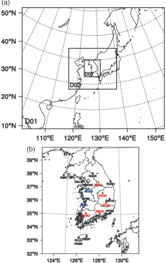
Figure 1.(a) Geographical areas of 54, 18, and 6 km domains. (b) Locations of radar observation sites operated by the Korea Meteorological Administration (KMA, black), Republic of Korea Air Force (ROKAF, red), and United States Air Force (USAF, blue) over the Korean Peninsula.
24 and 12-h forecasts for a 1-month period. Radar radial velocity and reflectivity observations from 19 stations (Figure 1(b)) over the Korean Peninsula are assimilated. All reflectivity observations greater than 0 dBZ are assimilated in this study. Before assimilation, radar data are preprocessed, including quality control, interpolation, and thinning. Details of the preprocess-ing of radar data can be found in Park and Lee (2009). Preprocessed radar data have horizontal, vertical, and temporal resolutions of 6 km, 0.5 km, and 10 min, respectively. Observation errors for radial velocity and reflectivity are assumed to be 2 m s−1 and 5 dBZ, respectively.
A total of 11 heavy rainfall cases over the Korean Peninsula, which occurred in 2006, 2008, and 2010 are selected. Selected heavy rainfall cases can be classified as isolated thunderstorm (IS), convection band (CB), cloud cluster (CC), or squall line (SL) according to Lee and Kim (2007). For each case, six experiments are con-ducted: NoDA, Rv, Rf, Rv+Rf, LS, and ERR. In the NoDA experiment, no radar data assimilation is car-ried out. In the Rv (Rf) experiment, only radial velocity (reflectivity) observation is assimilated, and both radial
velocity and reflectivity observations are assimilated in the Rv+Rf experiment. The LS experiment is the same as the Rv+Rf experiment except for employing tuned length scale, and the ERR experiment is the same as the LS experiment except for using tuned observa-tion error variance. Radar radial velocity and reflectiv-ity observations are assimilated using the methods of Xiaoet al.(2005) and Wanget al.(2013a), respectively. The length of the assimilation window is 30 min, and radar observations are available every 10 min within the assimilation window.
4. Results and discussions
For each case and experiment, a 24-h forecast is con-ducted, and the forecast starts 3 h before a heavy rain-fall system affects the Korean Peninsula. Because radar data assimilation is done only for the 6-km domain, the following analyses focus on the results of the 6-km domain.
4.1. Effects of assimilated variables
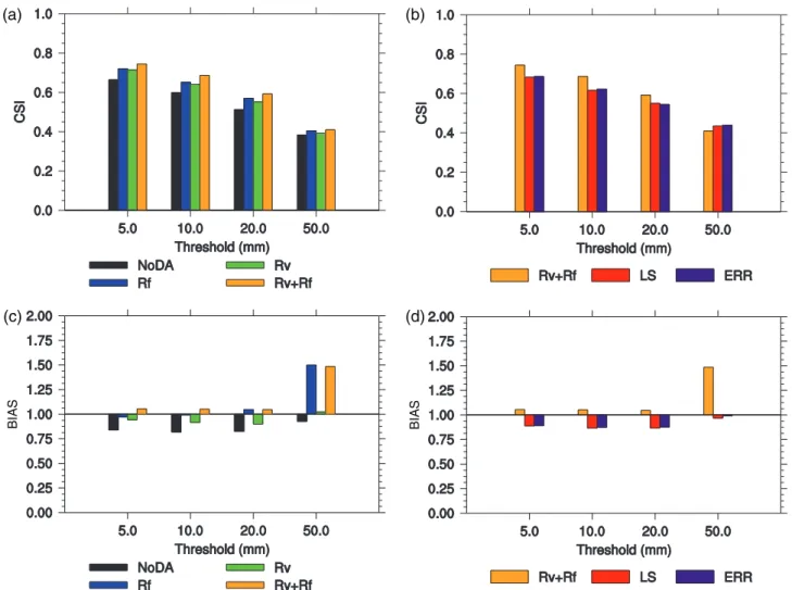
Figure 2 shows Critical Success Index (CSI) and frequency bias (BIAS) of 24-h accumulated rainfall amount for threshold values of 5, 10, 20, and 50 mm. For each experiment, CSI and BIAS values are aver-aged over 11 cases, and Automatic Weather Station (AWS) observations over the Korean Peninsula are used for verification. In order to investigate the effects of assimilated variables, CSI and BIAS values of the NoDA, Rf, Rv, and Rv+Rf experiments are compared in Figures 2(a) and (c). CSI and BIAS values of data assimilation experiments are better than those of the NoDA experiment, and this indicates positive effects of radar data assimilation on QPF skill. Regardless of threshold values, CSI of the Rf experiment is slightly greater than that of the Rv experiment. CSI values of the Rv+Rf experiment are better than those of the Rf experiment, and this implies that both kine-matic and hydrometeor information is important for improving QPF skill of heavy rainfall cases. Overall, the same conclusion can be drawn from the analy-ses of BIAS values. However, for 50-mm threshold, BIAS values of the Rf and Rv+Rf experiments are approximately 1.5, and this indicates that heavy precipitation is overpredicted in the Rf and Rv+Rf experiments.
4.2. Effects of length-scale tuning
Figure S1, Supporting Information shows O−B covari-ances from O−B statistics and Gaussian functions as a function of distance between two observations. O−B covariance from a Gaussian function with the length scale and background error variance determined using the method in Section 2.1 is plotted, and O-B covariances from Gaussian functions with different length scales are also plotted for comparison. Because
(a) (b)
(c) (d)
Figure 2.Critical Success Index (CSI) of 24-h accumulated rainfall amount for threshold values of 5, 10, 20, and 50 mm for (a) NoDA (black), Rf (blue), Rv (green), and Rv+Rf (orange) experiments and (b) Rv+Rf (orange), LS (red), and ERR (purple) experiments. Frequency Bias (BIAS) of 24-h accumulated rainfall amount for threshold values of 5, 10, 20, and 50 mm for (c) NoDA (black), Rf (blue), Rv (green), and Rv+Rf (orange) experiments and (d) Rv+Rf (orange), LS (red), and ERR (purple) experiments.
the original radar observations are thinned to 6-km mesh to remove spatial correlations between adjacent observations, O−B covariance from O−B statistics exists only for distances larger than 6 km. Although the observation error variance cannot be determined, the background error variance and length scale for background error covariance can be determined using the method in Section 2.1. Estimated length scales for radial velocity, rainwater, snow, and graupel are 7.7, 4.3, 4.5, and 4.0 km, respectively. For all observation types, O−B covariances from the fitted Gaussian func-tion represent O−B covariances from O−B statistics well. Note that length-scale values for stream function and velocity potential from the NMC-based statistics are about 90 and 70 km, respectively, and length-scales for rainwater, snow, and graupel are specified as a value of 6 km in the WRFDA system. Although length scale for radial velocity is estimated, length scales of control variables associated with wind (i.e. stream function and velocity potential) are tuned because data assimilation is done in control variable space in WRFDA.
In order to examine the effects of length-scale tun-ing, CSI and BIAS values of the Rv+Rf and LS
experiments are compared in Figures 2(b) and (d). For thresholds of 5, 10, and 20 mm, both CSI and BIAS of the Rv+Rf experiment are better than those of the LS experiment. However, for a threshold value of 50 mm, CSI and BIAS values of the LS experiment are better than those of the Rv+Rf experiment. In the Rv+Rf experiment, larger length scales than those in the LS experiment are used for the assimilation. Larger length scales in the Rv+Rf experiment spread the impact of radar observations to more distant grid points than the LS experiment, and this generally broadens simulated rainfall area. A broader rainfall area tends to give a better CSI value for small thresholds (i.e. weak rainfall), but it also produces erroneously wider area of weak rainfall [which leads to a higher Probability of False Detection (POFD) value]. POFD values (of 24-h accumulated rainfall) of the Rv+Rf experiment are greater than those of the LS experiment for all thresh-old values (see Figure S2). This stands out particularly at earlier forecast ranges. For earlier forecast ranges (1–9 h), BIAS values (of 1-h accumulated rainfall for 1-mm threshold) of the Rv+Rf experiment are much greater than those of the LS experiment (see Figure S2). Weak rainfall over wider areas simulated
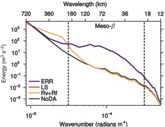
Figure 3.Vertically averaged (from 950 to 100 hPa) kinetic energy (m3s−2) spectra as a function of wavenumber (rad m−1) for analyses of NoDA (black), Rv+Rf (orange), LS (red), and ERR (purple) experiments.
in the Rv+Rf experiment makes CSI values higher for smaller thresholds, but it also leads to higher POFD values. This does not necessarily mean better fore-casts of heavy rainfall. Although QPF scores of the LS experiment are better than those of the Rv+Rf experiment only for the 50-mm threshold, this is still meaningful for weather forecasting given the difficul-ties in forecasting of severe weather events like heavy rainfall.
Kinetic energy (KE) spectra of analyses of the Rv+Rf and LS experiments are computed, and KE spectrum of the NoDA experiment is also calculated as a reference (Figure 3). For each case and experiment, the KE spectra from 950 to 100 hPa levels (with an interval of 50 hPa) are calculated and they are vertically averaged. And for each experiment, a total of 11 KE spectra from all heavy rainfall cases are averaged. The Discrete Cosine Transform (DCT) is used to compute KE spectra as in Denis et al. (2002). In the Rv+Rf experiment, energy at wavelengths between 120 and 720 km (i.e. mainly, meso-𝛼scale) is increased through radar data assimilation, compared with the NoDA experiment. In contrast, KE at wavelengths between 12 and 360 km (i.e. mainly, meso-𝛽 scale) is enhanced in the LS experiment compared with the NoDA experiment. Because selected heavy rainfall cases are related to meso-𝛽 or meso-𝛾 scale phenom-ena (e.g. squall line, mesoscale convective complex, convection band, and thunderstorm), the increase in KE at meso-𝛽 scale rather than meso-𝛼 scale is more reasonable.
To compare forecasts of the Rv+Rf and LS exper-iments, Root Mean Square Errors (RMSEs) of radial velocity and reflectivity are computed using 1-h fore-casts of the Rv+Rf or LS experiment and radar observations (Figure 4). For each case and experiment, hourly RMSEs of radial velocity and reflectivity are calculated for the forecast range of 0–24 h. Then, hourly RMSEs of radial velocity and reflectivity from
(a)
(b)
Figure 4.Root Mean Square Errors (RMSEs) of (a) radial veloc-ity (m s−1) and (b) reflectivity (dBZ) for forecasts of Rv+Rf (orange), LS (red), and ERR (purple) experiments. Error is defined as the difference between 1-h forecast and the cor-responding radar observations. Temporally averaged (0–24 h) RMSE value of each experiment is shown next to the experi-ment name.
11 cases are averaged for each experiment. From 0 to 11 h, RMSEs of radial velocity of the LS experiment are less than those of the Rv+Rf experiment. Similarly, RMSEs of reflectivity of the LS experiment are smaller than those of the Rv+Rf experiment for the forecast range of 0–12 h. In the LS experiment, by using the tuned length scales for radial velocity, rainwater, snow, and graupel when assimilating radar observations, the analyses fit better to the observations than the Rv+Rf experiment, and this improvement lasts for about 12 h.
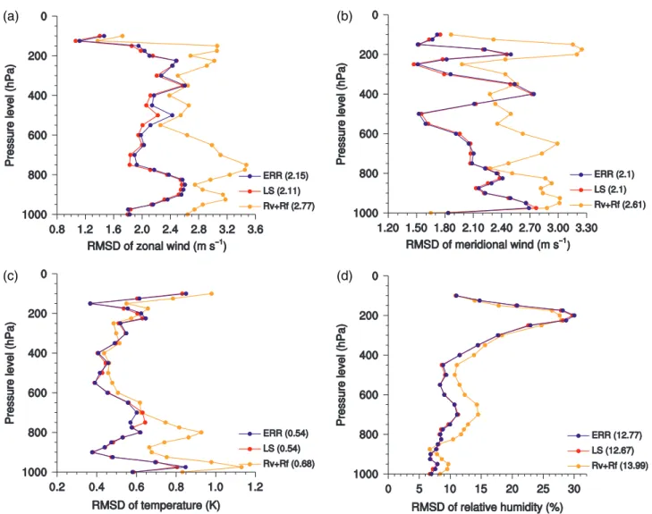
Finally, vertical distributions of RMS Differences (RMSDs) of zonal wind, meridional wind, temperature, and relative humidity are calculated using a 6-h fore-cast of the Rv+Rf or LS experiment (Figure 5). The forecast is verified against the ECMWF ERA-Interim data, and RMSDs from 11 cases are averaged. RMSDs of zonal and meridional winds of the LS experiment are smaller than those of the Rv+Rf experiment, espe-cially at lower-mid levels (i.e. 800–500 hPa). Similarly, RMSDs of relative humidity of the LS experiment are less than those of the Rv+Rf experiment at lower-mid levels. Although no temperature observations are assim-ilated, RMSDs of temperature are reduced in the LS experiment compared with the Rv+Rf experiment.
4.3. Effects of observation-error tuning
Observation errors for radial velocity and reflectivity are assumed to be 2 m s−1 and 5 dBZ, respectively,
(a) (b)
(c) (d)
Figure 5.Vertical distributions of RMS Differences (RMSDs) of (a) zonal wind (m s−1), (b) meridional wind (m s−1), (c) temperature (K), and (d) relative humidity (%) for 6-h forecasts of Rv+Rf (orange), LS (red), and ERR (purple) experiments. The ECMWF ERA-Interim reanalyses are used for verification. Vertically averaged (1000–100 hPa) RMSE value of each experiment is shown next to the experiment name.
and observation error for rainwater, snow, and grau-pel has a value between 0.0005 and 0.001 kg kg−1, depending on the corresponding mixing ratio. Tuning parameter for observation error can be obtained from the iterative process presented in Section 2.2. In order to help the observation error tuning parameter to con-verge, the background error tuning parameter is kept constant during the iterations. Table S1 shows obser-vation error tuning parameters as a function of itera-tion number. The observaitera-tion error tuning parameters for radial velocity, rainwater, snow, and graupel con-verge after 5, 4, 3, and 4 iterations, respectively. Con-verged tuning parameters for radial velocity, rainwa-ter, snow, and graupel are 0.97, 0.94, 0.91, and 0.91, respectively, and this implies a slight overestimation (3, 6, 9, and 9%) of observation error for all observed variables.
Although the difference is not large, CSI and BIAS values of the ERR experiment are better than those of the LS experiment for thresholds of 5, 10, and 50 mm (Figures 2(b) and (d)). RMSEs of radial veloc-ity and reflectivveloc-ity of the ERR experiment are similar to
those of the LS experiment (Figure 4). Similarly, verti-cal distributions of RMSDs of zonal wind, meridional wind, temperature, and relative humidity for the ERR experiment are close to those for the LS experiment (Figure 5). Overall, effects of observation-error tuning on QPF and wind/temperature/humidity forecasts are slightly positive and neutral, respectively. This may be because the computed tuning parameters for radial velocity, rainwater, snow, and graupel are close to one, and hence tuned observation errors are similar to the assumed ones. The improvement of QPF skill resulted from slightly changing observation errors implies that tuning of observation error can contribute to forecast improvements when the assumed observation error is not an optimal value.
5. Summary and conclusions
A total of 11 heavy rainfall cases over the Korean Peninsula are selected to investigate effects of tuning of length-scale and observation-error on heavy rain-fall forecasts. Radar radial velocity and reflectivity
observations are assimilated using the 4D-Var method, and the tuned length scale and observation error are applied. Length scale of background error correlation and observation error are tuned using the methods of Hollingsworth and Lönnberg (1986) and Desroziers and Ivanov (2001), respectively. The main conclusions of this study are as follows.
(1) Assimilation of both radial velocity and reflectivity results in better QPF skill than assimilation of either radial velocity or reflectivity. By assimilating both types of observations, kinematic and hydrometeor information can be added to the analysis.
(2) The use of tuned length scales leads to an analy-sis with more accurate meso-𝛽-scale information, reduced forecast errors of meteorological variables (i.e. wind, temperature, humidity, and hydrome-teor), and improved QPF skill for heavy precipita-tion.
(3) Effects of tuning of observation error on QPF skill and meteorological-variable forecasts are slightly positive and neutral, respectively. This is because the tuned observation errors are close to the assumed observation errors in this study. (4) Tuning of length-scale and observation-error is
important in assimilating radar observations using the 4D-Var method.
The findings of this study can contribute to the effec-tive use of radar observations, especially for fore-casting severe weather phenomena. The approaches for tuning length scale and observation error will be applied to AWS and satellite radiance observations in the future work.
Acknowledgements
This research was supported by the project of “Construction of a HPC-based Service Infrastructure Responding to National Scale Disasters (K-17-L03-C03)” in Korea Institute of Science and Technology Information (KISTI). The authors are thankful to associate editor, Dr. Ryan Neely and two anonymous reviewers for their valuable comments and suggestions.
Supporting information
The following supporting information is available:
Figure S1.O−B covariances from O−B statistics (bar), Gaus-sian functions with different length scales (line) as a function of distance for (a) radial velocity, (b) rainwater, (c) snow, and (d) graupel.
Figure S2.(a) Probability of False Detection (POFD) of 24-h accumulated rainfall amount for threshold values of 5, 10, 20, and 50 mm for Rv+RF (orange), LS (red), and ERR (purple) experiments. (b) Frequency Bias (BIAS) of 1-h accumulated rainfall amount for 1-mm threshold value for Rv+Rf (orange), LS (red), and ERR (purple) experiments. Temporal average of BIAS of each experiment is shown next to the experiment name.
Table S1.Observation error tuning parameters for radial veloc-ity, rainwater, snow, and graupel.
References
Barker DM, Huang XY, Liu Z, Auligne T, Zhang X, Rugg S, Ajjaji R, Bourgeois A, Bray J, Chen Y, Demirtas M, Guo YR, Henderson T, Huang W, Lin HC, Michalakes J, Rizvi S, Zhang X. 2012. The Weather Research and Forecasting (WRF) model’s community vari-ational/ensemble data assimilation system: WRFDA.Bulletin of the American Meteorological Society93: 831–843.
Buehner M, Gauthier P, Liu Z. 2005. Evaluation of new estimates of background- and observation-error covariances for variational assimilation.Quarterly Journal of Royal Meteorological Society131: 3373–3383.
Chapnik B, Desroziers G, Rabier F, Talagrand O. 2004. Properties and first application of an error-statistics tuning method in variational assimilation.Quarterly Journal of Royal Meteorological Society130: 2253–2275.
Chapnik B, Desroziers G, Rabier F, Talagrand O. 2006. Diagnosis and tuning of observational error in a quasi-operational data assimila-tion setting.Quarterly Journal of Royal Meteorological Society132: 543–565.
Denis B, C˘oté J, Laprise R. 2002. Spectral decomposition of two-dimensional atmospheric fields on limited-area domains using the Discrete Cosine Transform (DCT). Monthly Weather Review130: 1812–1829.
Desroziers G, Ivanov S. 2001. Diagnosis and adaptive tuning of observation-error parameters in a variational assimilation.Quarterly Journal of Royal Meteorological Society127: 1433–1452.
Desroziers G, Berre L, Chapnik B, Poli P. 2005. Diagnosis of obser-vation, background, and analysis-error statistics in observation space. Quarterly Journal of Royal Meteorological Society 131: 3385–3396.
Dudhia J. 1989. Numerical study of convection observed during the Winter Monsoon Experiment using a mesoscale two-dimensional model.Journal of Atmospheric Science46: 3077–3107.
Girard DA. 1989. A fast Monte Carlo cross-validation procedure for large least squares problems with noisy data.Numerische Mathematik
56: 1–23.
Ha JH, Lee DK. 2012. Effect of length scale tuning of background error in WRF-3DVAR system on assimilation of high-resolution surface data for heavy rainfall simulation.Advances in Atmospheric Sciences
29: 1142–1158.
Hollingsworth A, Lönnberg P. 1986. The statistical structure of short-range forecast errors as determined from radiosonde data. Part I: the wind field.Tellus38A: 111–136.
Hong SY, Lim JO. 2006. The WRF single-moment 6-class micro-physics scheme (WSM6).Journal of Korean Meteorological Society
42: 129–151.
Hong SY, Noh Y, Dudhia J. 2006. A new vertical diffusion package with an explicit treatment of entrainment processes.Monthly Weather Review134: 2318–2341.
Kain JS. 2004. The Kain-Fritsch convective parameterization: an update.
Journal of Applied Meteorology43: 170–181.
Lee JH, Lee HH, Choi Y, Kim HW, Lee DK. 2010. Radar data assimi-lation for the simuassimi-lation of mesoscale convective systems.Advances in Atmospheric Sciences27: 1025–1042.
Lee TY, Kim YH. 2007. Heavy precipitation systems over the Korean Peninsula and their classification.Journal of Korean Meteorological,
Society43: 367–396.
Lupu C, Cardinali C, McNally P. 2015. Adjoint-based forecast sensitiv-ity applied to observation-error variance tuning.Quarterly Journal of Royal Meteorological Society141: 3157–3165.
Mlawer EJ, Taubman SJ, Brown PD, Iacono MJ, Clough SA. 1997. Radiative transfer for inhomogeneous atmospheres: RRTM, a vali-dated correlated-k model for the longwave.Journal of Geophysical Research102: 16663–16682.
Park SG, Lee DK. 2009. Retrieval of high-resolution wind fields over the southern Korean Peninsula using the Doppler weather radar network.
Weather and Forecasting24: 87–103.
Parrish DF, Derber JC. 1992. The National Meteorological Center’s spectral statistical-interpolation analysis system. Monthly Weather Review120: 1747–1763.
Skamarock WC, Klemp JB, Dudhia J, Gill DO, Barker DM, Duda MG, Huang XY, Wang W, Powers JG. 2008. A description of the advanced research WRF version 3. NCAR Technical Note TN-475+STR, National Center for Atmospheric Research: Boulder, CO, USA, 113 pp.
Sun J. 2006. Convective-scale assimilation of radar data: progress and challenges.Quarterly Journal of Royal Meteorological Society131: 3439–3463.
Wang H, Sun J, Fan S, Huang XY. 2013a. Indirect assimilation of radar reflectivity with WRF 3D-Var and its impact on prediction of four
summertime convective events.Journal of Applied Meteorology and Climatology52: 889–902.
Wang H, Sun J, Zhang X, Huang XY, Auligné T. 2013b. Radar data assimilation with WRF 4D-Var. Part I: system develop-ment and preliminary testing. Monthly Weather Review 141: 2224–2244.
Xiao Q, Kuo YH, Sun J, Lee WC, Lim E, Guo YR, Barker DM. 2005. Assimilation of Doppler radar observations with a regional 3DVAR system: impact of Doppler velocities on forecasts of a heavy rainfall case.Journal of Applied Meteorology44: 768–788.