Fault Diagnostics of Dental X-ray
Systems
Harshit Agrawal
School of Science
Thesis submitted for examination for the degree of Master of Science in Technology.
Otaniemi 18.07.2018
Supervisor
Prof. Simo Särkkä
Advisor
Abstract of the master’s thesis
Author Harshit Agrawal
Title Deep Learning Methods for Visual Fault Diagnostics of Dental X-ray Systems Degree programme Life Science Technologies
Major Biomedical Engineering Code of major SCI3059 Supervisor Prof. Simo Särkkä
Advisor D.Sc. (Tech.) Kalle Karhu
Date 18.07.2018 Number of pages 64 Language English Abstract
Dental X-ray systems go through rigorous quality assurance protocols following their production and assembly. The protocols include tests which address the image quality and find certain errors or artifacts that may be present in the images. Detecting faults from the images require human effort, experience, and time. Recent advances in deep learning have proven them to be successful in image classification, object detection, machine translation. The applications of deep learning can be extended to fault detection in X-ray systems. This thesis work consists of surveying, applying, and developing state-of-art deep learn-ing approaches for detection of visual faults or artifacts in the dental X-ray systems. In this thesis, we have shown that deep learning methods can detect geometry and collimator artifacts from X-ray images efficiently and rapidly. This thesis is a precursor for further development of deep learning methods to include detection of wide range of faults and artifacts in X-ray systems to ease quality assurance, calibration, and device maintenance.
Keywords X-ray, CBCT imaging, deep learning, visual fault diagnostics, convolutional neural networks.
Preface
The machine learning and artificial intelligence revolution is moving forward faster than ever. Healthcare is not untouched from it. The latest machine learning ad-vances have potential to redesign healthcare completely. Being a customer service engineer for healthcare machines previously in India, I passionately dream about a world where healthcare is accessible to everyone with the lowest possible time and cost. This Master’s thesis work was done at Planmeca Oy, Helsinki, Finland. I would like to thank Planmeca Oy for the resources and the inspiring environment. I would like to thank thesis supervisor Professor Simo Särkkä for providing feedback and insights for writing this thesis. I thank thesis advisor Dr. Kalle Karhu at Planmeca for his guidance, proofreading, and helping attitude throughout the thesis. I am also grate-ful to the colleagues at Planmeca for bearing me and helping me out from time to time.
Otaniemi, 18.07.2018
Abstract 3 Preface 4 Contents 5 Abbreviations 6 List of Figures 7 List of Tables 11 1 Introduction 12 2 Background 15 2.1 Production of X-rays . . . 15 2.2 Computed tomography . . . 17
2.3 Cone-beam computed tomography. . . 18
2.4 Geometry and collimation artifacts . . . 23
2.5 Deep learning basics . . . 25
2.6 Overview of convolutional neural network . . . 29
3 Materials and Methods 36 3.1 Geometry artifacts . . . 36 3.1.1 Data acquisition. . . 36 3.1.2 Image preparation . . . 37 3.1.3 Network architecture . . . 37 3.2 Collimator artifacts . . . 40 3.2.1 Data acquisition. . . 40 3.2.2 Image preparation . . . 40 3.2.3 Network architecture . . . 40 3.3 Metrics . . . 44 4 Results 46 4.1 Geometry artifacts . . . 46 4.2 Collimation artifacts . . . 50 5 Conclusions 53 5.1 Summary . . . 53
5.2 Discussion and future work . . . 53
References 55
Abbreviations
Symbols
1D One dimensional 2D Two dimensional 3D Three dimensional
ADAM Adaptive moment estimation AE Autoencoder
API Application programming interface CBCT Cone-beam computed tomography CNN Convolutional neural network CPU Central processing unit CT Computed tomography DVT Digital volume tomography FDD Fault detection and diagnostics
FDK Feldkamp-Davis-Kress reconstruction algorithm FOV Field of view
GPU Graphics processing unit keV Kilo electronvolt
kVp Peak kilovolt LOO Leave-one-out
MRI Magnetic resonance imaging QA Quality assurance
R&D Research and development RBM Restricted Boltzmann machine ReLU Rectified linear unit
1 A simple schematic of X-ray tube (Pauwels et al., 2015). The cathode has negative and anode has positive charge. The filament in the cathode emits electrons, when heated. The focal spot makes a small portion of whole anode. The cathode electrons are accelerated towards anode. Whole process is carried out inside a glass envelope with vacuum. . . 15 2 Electron interaction with a target and its relationship to the X-ray
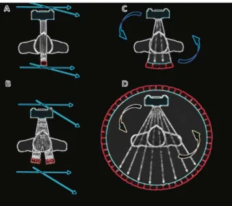
tube energy spectrum. (a) Bremsstrahlung radiation is produced when high-speed electrons are decelerated by the electric field of the target nuclei. (b) Characteristic radiation is generated when a high-speed electron interacts with a target electron and ejects it from its electronic shell. When outer-shell electrons fill in the vacant shell, characteristic X-rays are emitted. (c) A high-speed electron directly hits the nucleus and the entire kinetic energy gets converted to X-ray energy. For the X-ray spectrum shown in the figure, the target material is tungsten, and additional filtration is used to remove low-energy X-rays (Hsieh, 2015: p. 36). . . 16 3 The first generation CT scanners (A) utilized a pencil beam fixed
with a single detector moving simultaneously by translation-rotation motion. The second generation scanners (B) were similar to the first generation scanners but used multiple pencil beams coupled with multiple detectors and had a wider angle of rotation. The third generation scanners (C) utilized a fan-beam and an array of multiple detectors rotating simultaneously around the patient. The fourth generation scanners (D) used a wider fan-beam rotating around the patient and a stationary ring of multiple detectors (Mehr, 2013). . . 17 4 (A) Computed tomography utilizes a fan-shaped X-ray beam. (B)
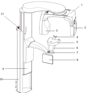
CBCT uses a cone-shaped X-ray beam. (Mehr, 2013). . . 18 5 Schematic drawing of Planmeca ProMax 3D CBCT device (Planmeca
Oy, 2017). Main parts of the machine are numbered as: (1) C-arm, (2) sensor (detector), (3) tube head, (4) patient supports, (5) patient support table, (6) patient handles, (7) patient positioning controls, (8) touch screen, (9) telescopic column, (10) stationary column, (11)
emergency stop button. . . 19 6 An X-ray beam passing through an object with different attenuation
coefficients along a line.. . . 19
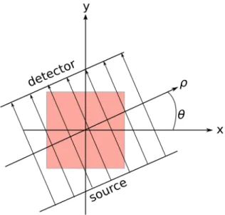
7 The parallel projection geometry. The source and detector rotate about the center of the object. For each angle θ, the attenuation coefficients are added along the X-ray at the detector. Projections are usually taken for the θ∈[0,180). . . 21 8 Ideal Feldkamp geometry. The X-ray source S rotates along an ideal
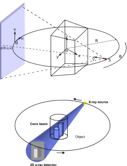
circle of radiusR with center of rotation at O. In this geometry, the rotation direction is anti-clockwise and given by the angle θ. The detector is on the opposite side and rotates along with the source in the same direction. The lower diagram is a simpler representation of cone-beam geometry (Sakamoto et al., 2005). . . 22 9 Upper two images show the motion artifact and the lower two images
are without any motion artifacts. The images have been acquired on a skull phantom at the R&D facility of Planmeca Oy. . . 24 10 Upper two images show the collimation artifact in the extended
volume and the lower two images are without any collimation artifacts. The images have been acquired on a skull phantom at the R&D facility of Planmeca Oy. . . 25 11 Flowchart of collimation calibration in the production. The process
is repeated until the collimator artifacts are not visible any more in the extended volumes. . . 26 12 The upper diagram is a biological neuron and the lower diagram is
equivalent model of the perceptron (Li, 2018). . . 27 13 The left diagram is sigmoid, middle is tanh, and right is ReLU
non-linearity (Li, 2018).. . . 28 14 A simple feed-forward neural network with one hidden layer. . . 29 15 LenNet-5 network (LeCun et al., 1998). The convolution of 6 filter
kernels with the input image of 32×32 results in 6 feature maps of size 28×28 (C1). In next layer S2, average pooling (subsampling) is performed using a 2×2 kernel. Again a convolution (C3) and pooling (C5) was performed. Now the map values are flattened and two fully connected layers (C5, F6) are attached. The output layer has 10 units for 10 classes. . . 30 16 2-D Convolution. f is a 2-D image which is convolved with the filter
kernelg. The center pixel 5 showed inside the red box in the input image gets changed to -45 in the output imageh after convolutional operation. . . 31 17 Maxpooling. . . 32
18 One of the phantom set up used to acquire the training data with Promax mid CBCT device (Courtsey of Planmeca Oy). . . 37 19 The left image is an input image of size 268×268 and the right
image shows 64 patches of size 60×60 made from the left image with 50% overlap. . . 38 20 The convolutional neural network with three hidden layers, one fully
connected layer and one softmax layer as output. The size of input isH×W×D, where H is height, W is width and Dis depth of the input. In our experiment, the input size is 60×60×1. The outputs of the network are the probabilities for the two classes, in our case, motion and non-motion (Küstner et al., 2018) . . . 38 21 The original VGG-16 network with 16 layers (Simonyan and
Zis-serman, 2014). The output softmax layer has 1000 units for 1000 classes in ImageNet database. . . 41 22 The VGG-16 architecture showing different layers and parameters.
The softmax layer has 1000 units for 1000 class classification in ImageNet data. . . 41 23 The custom VGG architecture showing different layers and
parame-ters. The softmax layer has 2 units for 2 class classification.. . . 43 24 The accuracy and loss curves during model training. . . 46 25 The motion maps for some test images. The left images show the
probability of motion for patches of the right images projected back into the image space with an patch overlap of 50%. The patches more than 55% zero pixels have been given 0 probability by default. (A) is canine motion image with 96% motion patches. (B) is canine
non-motion image with 0% motion patches. (C) is temporal bone motion image with 32% motion patches. (D) is temporal bone non-motion image with 0% non-motion patches. (E) is jaw non-motion image with 38% motion. (F) is jaw non-motion image with 1% motion patches. The colorbar is shown on the top. . . 49 26 Change in slice-wise accuracy and prediction time for different
num-ber of slices. We took different slices from each volume and the model predicted artifact/no artifact for each slice. Even with 10 slices from 65 volumes, the accuracy is 96.7% and the prediction time is only 6.4 seconds. . . 50
27 Change in volume-wise accuracy and prediction time for different number of slices. We took different slices from single good volume and the model predicted artifact/no-artifact for single volume. With 10 slices from the volume, prediction time is only 0.13 seconds and accuracy is still 100%. . . 51 28 Accuracy and loss curves during training of custom model with
dropout. . . 51 29 Activations in the first convolutional layer (upper), and the last
convolutional layer (lower) of the trained custom model applied on a collimator artifact image. Every box represents an activation map corresponding to some filter. Activations are dense in the first layer but sparse in the last layer capturing arc like artifact. . . 52
1 Slice-wise test accuracy for the canine and temporal bone images. 200 with motion and 200 without motion canine images and 400 with motion and 400 without motion temporal bone images were used for testing of the model. We had 800 with motion and 800 without motion slices from jaw volumes. . . 47 2 Volume-wise motion detection accuracies for two canine volumes.. . 47 3 Volume-wise motion detection accuracies for temporal bone volumes. 47 4 Volume-wise motion detection accuracies for each jaw volume. . . . 48 5 Various scores for the canine, temporal bone and jaw image slices.
Class 0 slice is without artifact and class 1 slice is with motion artifact. 48 6 Accuracy and loss for training, validation, and testing. Testing
results are for 6500 slices. "dp" stands for dropout and "aug" is data augmentation. . . 50
Dentistry has seen tremendous advances over the past three decades. The need for more precise imaging and diagnostics tools has become essential (Shah et al., 2014). X-ray based techniques are playing a major role in the development of these tools. From simple intra-oral periapical X-rays to more advanced extra-oral imaging techniques like fan-shaped X-ray beam based computed tomography (CT) or cone-shaped X-ray beam based cone-beam computed tomography (CBCT) are being used in dental applications (Vandenberghe et al., 201).
Current state-of-art CBCT systems provide excellent high resolution and three dimensional images of oral bony anatomy. CBCT scans are also low cost in comparison to CT scans. However many imaging artifacts are inherently present in CBCT systems (Nagarajappa et al., 2015; Schulze et al.,2011). These artifacts may contribute to
image degradation and lead to inaccurate or false diagnostics (Lee, 2008).
Before being delivered to the diagnostics facility, dental X-ray systems go through rigorous quality assurance (QA) protocols following their production and assembly. Many of these tests still require a lot of human intervention. The human operator has to go through many image volumes and decide the quality of the images based on his/her experience, which if automated, could save many work hours and improve the decision making accuracy. In addition, the image quality of the system may change with the wear and tear in various machine parts during the usage at the diagnostics facility. It will be beneficial to have a mechanism to monitor the degradation of image quality and its causes automatically. This would enhance customer experience and reduce number of visits of service engineer to the diagnostics facility.
Recent advances in machine learning methods for image classification and pattern recognition provide excellent precursor for the visual fault detection task. Notably deep learning and large convolutional neural network models (Alex et al., 2012; Simonyan and Zisserman, 2014) have recently demonstrated impressive image clas-sification performance on the ImageNet large scale visual recognition challenge benchmark, an international competition for object detection and classification, consisting of 1.2 million everyday color images (Russakovsky et al., 2015).
The purpose of this thesis is to investigate applicability of state-of-art deep learning methods for the automatic detection of various visual faults in dental X-ray systems in order to ease tests at production or during service. This will provide better and improved quality services to the customer. This work mainly focuses on testing the classification of artificially induced geometry and collimator artifacts in the images generated using skull phantoms. We demonstrate that good accuracies can be obtained for visual faults detection using deep learning methods.
Prior work
Fault detection and diagnostics (FDD) have been an important aspect from shipping (Babaei et al., 2018) to aircraft Glavaski and Elgersma (2001) industries and from building systems (Katipamula and Brambley,2005b) to medical equipment (López et al., 2009). The primary objective of an FDD system is early detection of faults
and diagnosis of their causes, enabling corrections before additional damage to the system or loss of service occurs as described byKatipamula and Brambley(2005a) for building systems. In the case of medical equipment, safety of patient becomes another important factor. It is better if the faults in medical equipment could be detected during the production phase itself as it minimizes the costs and safety concerns arising from the bug fixing and recalls in later phases (Alemzadeh et al., 2013). The faults may also occur later during the usage at customer sites due to wear and tear in the equipment. The dental X-ray systems are also tightly regulated to avoid radiation overdose to the patient or repeated exams (Hirvonen-Kari, 2013; Rout and Brown, 2013). Thus the fault detection or even fault prediction becomes a crucial aspect for medical equipment.
The FDD systems can be divided into two major categories: model based and data driven. In model based methods, domain knowledge of the system is incorporated to create a model and the measured values of some system parameters are compared with the model values and prediction is made (Isermann, 2005; Oppenheimer and Loparo,2002). The complexity and noisy working conditions affect the development of such models and most of these models can not be updated with on-line measured data (Zhao et al.,2016b). On the other hand, data driven fault detection models learn a model based on observations of input and output data (Katipamula and Brambley, 2005a). These methods have become more attractive because of availability of big data, large computing power, and breakthrough of deep learning (Zhao et al.,2016b). The faults in an equipment can be mechanical (Sheng et al., 2011) or software specific (Wallace and Kuhn, 2001, 1999). Depending upon the type of the fault and data available for the model training, different approaches are used. There have been many recent attempts to detect machine faults by applying deep learning methods (Zhao et al., 2016b). Sun et al. (2016) proposed a one layer autoencoder (AE,Goodfellow et al.,2016a) based neural architecture for the classification of faults in induction motor. They classified six types of the motor conditions using vibration signals acquired by an acceleration sensor. Lu et al.(2017) presented a detailed study of stacked denoising autoencoders with three hidden layers for fault diagnosis of rotary machinery components. The input features to those autoencoder models were raw sensory time-series. In Deutsch and He (2017), a restricted Boltzmann machine (RBM,Smolensky,1986) based method was proposed for the prediction of remaining useful life of a bearing. Ding and He (2017) proposed a deep convolutional network where wavelet packet energy images were used as input for spindle bearing fault diagnosis. Recurrent neural network (RNNRumelhart et al.,1986b) (RNN) models are used to handle sequential data with its ability to encode temporal information. The RNN models have been applied in various machine health monitoring problems recently (M.Yuan et al.,2016; Zhao et al., 2016a).
The progress in deep learning methods is changing the analysis of natural images (Dong et al.,2016) and videos (Wang et al.,2015). Similar examples are emerging in medical imaging. In the image related problems, convolutional neural networks have been used extensively. Litjens et al. (2017) have stated that out of the 47 papers published on medical image classification in 2015, 2016, and 2017, 36 were using CNNs, 5 AEs, and 6 were using RBMs. The application areas of these methods
were very diverse, ranging from brain magnetic resonance imaging (MRI) to retinal imaging and digital pathology to lung computed tomography (CT). Examples include classification of pulmonary tuberculosis from X-ray images (Lakhani and Sundaram, 2017), X-ray scattering image classification (Wang et al., 2017), differential diagnosis of benign and malignant breast nodules from ultrasound images (Cheng et al., 2016), and identifying diabetic retinopathy in retinal fundus photographs (Gulshan et al., 2016).
Similarly, CNNs have been used recently to detect artifacts in medical images. Meding et al. (2017) implemented a convolutional neural network for automatic detection of motion artifacts in MRI images. The network architecture consisted of two sequential convolutional layers interleaved with ReLU and pooling layers. Küstner et al. (2018) used a patch based approach for detection of motion artifacts from MRI images. They divided image slices to patches and fed the patches to the CNN. Zhang and Yu (2018) used convolutional neural network based approach for metal artifact reduction in CT scan images. Granholm (2018) tried transfer learning based CNNs for the detection of geometry and collimation artifacts from calibration images in CBCT machines.
Structure of the thesis
We start by describing the basics of X-ray production and main principles behind CBCT scanning. We then briefly explain motion and collimation artifacts in CBCT machine. We explain the central concepts in deep learning with focus on convolutional neural networks. Then we describe the neural network architectures and data collection methods used in our work. We also provide the code snippets wherever required. Finally we show the results obtained in our experiments and discuss how the deep learning methods can reduce the workload in the production and enhance accuracy for the visual fault diagnosis in dental X-ray systems.
2
Background
Since the revolutionary invention of X-rays in 1895 by Roentgen (Glasser, 1995), many diagnostics and imaging techniques have been developed such as digital X-ray, computed tomography (CT Scan), mammography, cath-lab. One such technique is cone-beam CT (CBCT), which is also known as digital volumetric tomography (DVT). Commercial development of dental CBCT technology first emerged in second half of the 1990s (Glasser, 1995; Mozzo et al., 1998; Arai et al., 1999; Scarfe and Farman, 2007;Scarfe et al.,2012). CBCT machines have been a widely used tool for several dental applications such as implant planning (implantology), endodontics, oral and maxillofacial surgery, and orthodontics (Scarfe et al., 2007, 2009; Mehr, 2013; Harrel Jr et al., 2018; Doyle et al., 2018; Alamari et al., 2012). Below we describe some basic principles and background physics behind X-ray and CBCT devices.
2.1
Production of X-rays
X-rays are generated in a glass tube containing two oppositely charged electrodes. Positively charged electrode is called anode and the negatively charged electrode is called cathode. Both electrodes are separated by a vacuum. The cathode consists of a filament which when supplied an electric current, gets heated and emits electrons. This process is called thermionic emission. A high voltage of the order of thousands of volts is applied between the two electrodes to accelerate the cathode electrons towards the anode. The area of the anode surface which receives the beam of electrons from the cathode is called focal spot. The focal spot consists of a high density material (e.g. tungsten). When the high speed electrons collide with the target material (focal
spot), X-rays are produced (Bushberg et al.,2012a; Hsieh,2015: pp. 33–42).
Figure 1:A simple schematic of X-ray tube (Pauwels et al.,2015). The cathode has negative and anode has positive charge. The filament in the cathode emits electrons, when heated. The focal spot makes a small portion of whole anode. The cathode electrons are accelerated towards anode. Whole process is carried out inside a glass envelope with vacuum.
input energy gets converted into heat. There can be three types of the interaction of the speeding cathode electrons with the target atoms as described in Hsieh (2015: p. 35). The high-speed electron travels partially around the nucleus due to the attraction between the positive nucleus and the negative electron. The sudden deceleration of the electron produces Bremsstrahlung radiation and energy of this Bremsstrahlung radiation depends on the kinetic energy of the incident electron which is given off in de-acceleration. As the amount of interaction increases, the resulting X-ray energy increases. This type of radiation covers the entire range of the X-ray energy spectrum. If the electron collides directly with a nucleus, its entire energy appears as Bremsstrahlung. The X-ray energy produced by this interaction represents the upper energy limit in the X-ray spectrum. For example, for an X-ray tube operating at 120 kVp, this interaction produces X-ray photons with 120-keV energy. This kind of interactions are very rare. The third kind of interaction occurs when a high-speed electron collides with one of the inner shell electrons of the target atom and frees the inner shell electron. When the hole is filled by an electron from an outer shell, characteristic radiation is emitted. The energy of the characteristic X-ray is the difference between the binding energies of two shells.
Figure 2: Electron interaction with a target and its relationship to the X-ray tube energy spectrum. (a) Bremsstrahlung radiation is produced when high-speed electrons are decelerated by the electric field of the target nuclei. (b) Characteristic radiation is generated when a high-speed electron interacts with a target electron and ejects it from its electronic shell. When outer-shell electrons fill in the vacant shell, characteristic X-rays are emitted. (c) A high-speed electron directly hits the nucleus and the entire kinetic energy gets converted to X-ray energy. For the X-ray spectrum shown in the figure, the target material is tungsten, and additional filtration is used to remove low-energy X-rays (Hsieh, 2015: p. 36).
2.2
Computed tomography
Computed tomography (CT) is a technique for imaging cross-sections of an object using a series of X-ray measurements taken from different angles around the object. CT uses simultaneously rotating detectors and X-ray tube. The development of the CT technology is often divided into four generations (Goldman, 2007; Bushberg et al.,2012b).
The first-generation of CT consists of X-ray tube rigidly linked to a detector located on the other side of the subject. The tube-detector sweeps horizontally which is called translation. During translation, the measurement is made at each location of the detector using a pencil beam X-ray. Then the system rotates at 1◦ increments to collect 180 views over 180◦ rotation.
The second-generation CT used multiple narrow beams of X-rays with multiple detectors and, as in the first generation, used rotate–translate motion. Number of required translations was reduced by a factor of 1/(number of detectors) (Goldman, 2007).
The third-generation CT eliminates translation and motion is purely rotation using slip-ring technology. The X-ray beam is fan-beam. This form of CT technology is most commonly used currently.
The fourth-generation CT consists detectors placed circularly and rapid measure-ments are taken as the tube sweeps across the field of view of the detector. Because of expensive detector arrays, the fourth-generation CT scans did not gain popularity.
Figure 3: The first generation CT scanners (A) utilized a pencil beam fixed with a single detector moving simultaneously by translation-rotation motion. The second generation scanners (B) were similar to the first generation scanners but used multiple pencil beams coupled with multiple detectors and had a wider angle of rotation. The third generation scanners (C) utilized a fan-beam and an array of multiple detectors rotating simultaneously around the patient. The fourth generation scanners (D) used a wider fan-beam rotating around the patient and a stationary ring of multiple detectors (Mehr, 2013).
2.3
Cone-beam computed tomography
CBCT has revolutionised dental diagnosis by facilitating transition from 2D imaging to 3D imaging, which has added a lot of third party applications. The traditional CT scan systems used a fan-shaped beam and several detectors to acquire individual image slices of the field of view (FOV) and then stack the slices to obtain a 3D representation. CBCT uses a cone-shaped beam and a single detector where X-rays are directed through the middle of the area of interest onto the detector on opposite side. The X-ray source and the detector rotate around the patient and take multiple sequential projection images of the field of view (FOV). Only one rotation sequence of the gantry is necessary to acquire enough data for image reconstruction (Farman and Scarfe, 2018).
Figure 4: (A) Computed tomography utilizes a fan-shaped X-ray beam. (B) CBCT uses a cone-shaped X-ray beam. (Mehr, 2013).
CBCT scan has smaller size and lower cost in comparison to CT scan. Since CBCT aquires data from whole FOV, it has faster scan time which results in the reduction of image unsharpness caused by the translation of the patient, reduced image distortion due to internal patient movements, and increased X-ray tube efficiency (Gulsahi, 2011). However, because of larger FOV, large amounts of scattered radiation is produced. The detection of large scattered radiation in CBCT causes limitations in image quality related to noise and contrast resolution (Scarfe and Farman, 2008). Nonetheless, CBCT has become a popular tool for dental and maxillofacial imaging (Jacobs, 2011; Mamatha et al., 2015).
A CBCT device is shown in Figure 5. In CBCT device, a C-shaped rotating arm (C-arm) consists of a radiation source (X-ray tube) and a detector mounted on opposite side. The target object (patient or phantom) is placed between the X-ray source and detector. During a scan, the C-arm rotates in a circular trajectory around the target object, collecting hundreds of frames (views) from different angles. The frames are sent to a computer for reconstruction, which computes a 3D reconstruction of the target object.
Figure 5: Schematic drawing of Planmeca ProMax 3D CBCT device (Planmeca Oy, 2017). Main parts of the machine are numbered as: (1) C-arm, (2) sensor (detector), (3) tube head, (4) patient supports, (5) patient support table, (6) patient handles, (7) patient positioning controls, (8) touch screen, (9) telescopic column, (10) stationary column, (11) emergency stop button.
Image reconstruction
When an X-ray travels through an object, it attenuates due to effects such as absorption or refraction (McKetty, 1998). The internal material of the object has an absorption coefficient at each point in the space, higher attenuation coefficient implies a denser material.
Figure 6: An X-ray beam passing through an object with different attenuation coefficients along a line.
If we assume that X-ray is infinitely thin and travels along a straight line (see Figure6), the relationship between the incident intensity of X-raysIinand transmitted
intensityIout can be written according to Beer-Lambert law (Swinehart,1962),
Iout =Iin exp[− ∫ L
0
µ(l)dl], (1)
where µ(l) is attenuation coefficient of the object in the beam path. By taking logarithm on both sides, the line integral can be written as,
p= ∫ L 0 µ(l)dl=−lnIout Iin , (2)
where p is the projection measurement and L is the thickness of the object X-ray beam travelled.
This can be extended to a 2D object (image slice) as shown in Figure7 where X-ray projections are taken along many parallel lines. In a parallel projection geometry, parallel projections are also taken at several angles θ. The source and detector move together in a circular path. For the purpose of CT, the inside of the object can be reconstructed by obtaining attenuation coefficients or the object density information. If the object’s densities are represented by a function f(x, y), the line projections can be written as,
p(ρ, θ) =
∫ ∞
−∞
∫ ∞
−∞f(x, y)δ(xcosθ+ysinθ−ρ)dxdy, (3)
where projectionp(ρ, θ) is also called forward Radon transform of the object function
f(x, y), ρ = xcosθ+ysinθ is line along the projections, and δ(.) is Dirac delta function (Kak and Slaney, 1988b: p. 50).
The task is to construct the image of the object by obtaining inverse Radon transform using such projection measurements. Two major categories of reconstruc-tion methods are analytical and iterative. In general, analytical reconstrucreconstruc-tion is considered computationally more efficient while iterative reconstruction can improve image quality (Hsieh et al., 2013). Traditionally, most commonly used analytical reconstruction method in commercial CT scanners has been filtered back-projection (FBP) (Saxena and Kumar,2018). It applies a 1-D filter on the projection data before back-projecting (smearing) the data onto image space (Hiriyannaiah, 1997; Kak and Slaney, 1988b). Various FBP-type methods have been developed for different generations of CT scans. The detailed explanation of these methods is not in the scope of this thesis but the curious reader can refer to the book by Kak and Slaney (1988a) for fundamentals of image reconstruction and review by Flohr et al.(2005)
for multi-slice CT reconstruction.
Feldkamp algorithm
In CBCT the detector is 2D and projections could be considered as 2D forward Radon transforms. While there have been many variants developed for the image reconstruction as described byTurbell (2001), for a simple and fast implementation, the well known Feldkamp algorithm is mostly used either in its original form ( Feld-kamp et al.,1984) or with some modifications (Xiao et al., 2003; Scherl,2012). We
Figure 7: The parallel projection geometry. The source and detector rotate about the center of the object. For each angle θ, the attenuation coefficients are added along the X-ray at the detector. Projections are usually taken for theθ ∈[0,180).
will explain Feldkamp algorithm in simple form here. For more detailed explanation and derivations, reader can consult (Feldkamp et al., 1984; Turbell, 2001).
The Feldkamp algorithm (FDK) is based upon a circular trajectory (see Figure 8), where the source and detector rotate along an ideal circle. The X-ray source S is at a distanceD from the detector center d. The object in the middle is in the world coordinate system (x, y, z) placed at the rotation center O. OX is aligned towards the source and detector center at angle zero. The flat panel detector and source rotate together around thez-axis. The radius of the circular trajectory is R, and u
andv are the pixels in the image. For any ray hitting the detector at u andv at a particular angleθ, the projection function can be written as,
p(θ, u, v) =
∫ ∞
0
f(s(θ) +αγˆ)dα, (4) wheres(θ) = (Rsinθ, Rcosθ,0) is the location of the source with respect to rotation center O, α ∈ [0,√D2+u2+v2] is the distance from source along the ray vector
and ˆγ is the unit vector along the direction of ray vector (Scherl,2012).
Steps: FDK is an approximate reconstruction algorithm. FDK algorithm for circular CBCT with planar detector can be applied in following successive steps: Step 1 - Filtering: Each measured projection p(θ, u, v) is filtered in following steps:
(a) Cosine weighting: This step weights the projections according to the cosine of the angleϕ between the ray hitting the detector at center d and the ray hitting the
Figure 8:Ideal Feldkamp geometry. The X-ray source S rotates along an ideal circle of radiusR with center of rotation at O. In this geometry, the rotation direction is anti-clockwise and given by the angle θ. The detector is on the opposite side and rotates along with the source in the same direction. The lower diagram is a simpler representation of cone-beam geometry (Sakamoto et al., 2005).
detector at (u, v).
pc(θ, u, v) = p(θ, u, v)×cosϕ, (5)
where cosϕ = √ D
u2+v2+D2.
(b) Ramp filtering: This step is 1-D convolution along the rows of the detec-tor The cosine-weighted projections are convolved with a ramp filter (Wei et al., 2005).
pf(θ, u, v) =pc(θ, u, v)∗h(u), (6)
Step - 2 Back-projection: The filtered projections are back-projected (smeared) into the image space to obtain approximated solution as below.
ˆ
f(x, y, z) =
∫ 2π
0
µ(θ, x, y, z)pf(θ, u(θ, x, y, z), v(θ, x, y, z))d(θ), (7)
where µ(θ, x, y, z) is a point-dependent distance weight such as,
µ(θ, x, y, z) = R
2
R+ysinθ−xcosθ, (8)
and the detector coordinates u and v in terms of x, y, z coordinate system (Xiao et al.,2003) are,
u(θ, x, y) = D(ycosθ+xsinθ)
R+ysinθ−xcosθ, (9)
v(θ, x, y, z) = zD
R+ysinθ−xcosθ. (10)
2.4
Geometry and collimation artifacts
Geometry artifactsIn reality, the assumption of a circular source-detector trajectory is not essentially true. Motion of the X-ray source and detector differ significantly from a simple circular orbit (Daly et al.,2008) due to, for example, gravity-induced mechanical flex (Jaffray et al., 2002) or due to the tilted detector rows with respect to an ideal Feldkamp-like acquisition (Scherl, 2012). Failing to correct such non-idealities may result in misregistration, loss of details, or image artifacts (Jaffray et al., 2002). A calibration of the imaging system geometry is done for the accurate image reconstruction (Yang et al.,2006).
In geometry calibration, a specific phantom with known dimensions is scanned and various geometry parameters are recorded. During the reconstruction, the geometry parameters already obtained from the calibrations are in the reconstruc-tion algorithm (Cho et al., 2005; Yang et al., 2006). During the patient scan, it is assumed that the patient is stationary and the source and detector are follow-ing a predefined trajectory. The motion artifacts can occur from one of the two causes: 1. Patient motion: The exposure time in CBCT ranges from 5.4 to 40 seconds (Nemtoi et al., 2013) and such time is long enough for the patient’s movements.
Hanzelka et al. (2013) have found that patient with open eyes tend to follow the motion of the C-arm. Patient motion can cause misregistration artifacts within the image (Lee,2008). If an object moves during the scanning process, the reconstruction algorithm does not account for the movement since no information on this movement is integrated in the reconstruction process.
2. Non-patient motion: If the geometry defined in the geometry calibration files does not repeat itself due to some reason like flex or jitters while rotation, it can
cause motion artifacts in the images (Jaffray et al., 2002). This causes same sort of artifacts as described above. Reconstruction algorithms try to compensate those effects up to some limit. It is not essential that the source and detector follow a perfect circular trajectory, but the trajectory should be repeatable following the geometry calibration (Pauwels et al., 2015). Even minute deviations can cause poor image quality (Nagarajappa et al., 2015).
Motion artifacts can have detrimental impact on the diagnostic images. It is beneficial to be aware of the presence of artifacts and be familiar with their characteristic appear-ances in order to enhance the extraction of diagnostic information from cone-beam images (Makins,2014;Nardi et al.,2016).
Figure 9: Upper two images show the motion artifact and the lower two images are without any motion artifacts. The images have been acquired on a skull phantom at the R&D facility of Planmeca Oy.
Collimation artifacts
The collimator is essentially a rectangular window made from lead sheets. It controls the field of view for the X-ray exposure. If the collimator window is not open accurately during the scan, it can cause the artifacts in the images. In the production, extended volumes are taken in order to visualise the collimation artifacts more clearly. The worker has to go through all the images in the extended volume manually and decide whether there is artifact. If there is an collimation artifact, worker needs to move the collimator manually and repeat the whole process again.
Collimator calibration pipeline in production: In order to check and do the collimation calibration the CBCT device goes through the work-flow shown in Figure 11. Beam check is done to see whether the collimator is open enough to cover the rectangular detector. The flat field calibration is done for the correction of the pixel
Figure 10: Upper two images show the collimation artifact in the extended volume and the lower two images are without any collimation artifacts. The images have been acquired on a skull phantom at the R&D facility of Planmeca Oy.
gain and dark currents in the detector when no object is present between source and detector. After this, the extended volume scan is taken on a skull phantom to check if any collimator artifact is visible in the images. If the collimator artifact is visible, the collimator blades are moved wider and the whole process is repeated again until the collimator artifacts are not visible. Once there are no collimator artifacts, other scans and checks can be performed.
2.5
Deep learning basics
Machine learningClassical computer programs are explicitly programmed by hand to perform a task. With machine learning, some part of the human contribution is replaced by an algorithm. In machine learning, computers are fed with data and the computer algorithm tries to learn the hidden relationships in the data (Bishop,2006; Murphy, 2012).
In supervised machine learning (Hastie et al., 2008a), the program receives a set of inputs and corresponding labels as training dataset and the algorithm tries to learn the relationship between input and output. Once the algorithm is trained, it can predict an output for any new input. In unsupervised machine learning (Hastie et al., 2008b), there is no training dataset, but the task of the computer is to divide the input data into a number of clusters or to find patterns. In supervised learning, we are interested in the prediction of the output class for an input rather than making clusters of inputs whose labels are unknown. For example, in a typical cat-dog classification problem, if a dataset is available with images of dogs and cats and the corresponding labels, supervised learning can be used to learn the relationship
Figure 11: Flowchart of collimation calibration in the production. The process is repeated until the collimator artifacts are not visible any more in the extended volumes.
between the images and labels. The trained network will predict the label for any new image of cat or dog. On the other hand, unsupervised learning will need no labelled data. Unsupervised learning will try to separate the input cat and dog images into two separate clusters, but the label of the both clusters will not be available.
In this work, the focus is in the applications of deep learning (Goodfellow et al., 2016b), a subset of machine learning. Deep learning is a branch of machine learning which has become very popular in recent years for its wide range of applications (Voulodimos et al., 2018; Ker et al., 2018). Below we will describe some central
concepts in deep learning which we have utilized in our work. Neuron model
The basic unit of the neural network is loosely motivated by the basic computational unit of the brain called neuron. The early model of a neuron is termed as McCulloch Pitts neuron (McCulloch, 1943). There are approximately 100 billion neurons in the human brain and each neuron is estimated to have up to 15,000 connections with other neurons (Nguyen, 2013). Each neuron receives input signals from the connected neurons at its dendrites. The input signals get summed and if the total sum is above a certain threshold, the neuron can fire, sending a spike along its axon.
The firing of the neuron is called activation and there are many activation functions which are used in practice nowadays, which are different from the classical (binary) neuronal model. The output can be expressed in mathematical form as,
output=ϕ(
m ∑
m=1
Figure 12: The upper diagram is a biological neuron and the lower diagram is equivalent model of the perceptron (Li, 2018).
where wm are the weights of the m connected neurons, b is the neuron bias, and ϕ is
the activation function.
These neuronal units are essentially not the same as in the brain. There are many different types of neurons with very different characteristics. For example, synapses are not just simple scalar weights but they are complex non-linear and dynamic system (London and Häusser,2005;Brunel et al.,2014). The McCulloch-Pitts neuron could fire (0,1) or (-1,1). However, this model is so simplistic that it only generates a binary output. Nevertheless, below are some popular activation functions.
Activation functions
The capacity of the neural networks to approximate any function, especially non-convex, is directly the result of the non-linear activation functions. Activation function takes a vector and performs a certain fixed point-wise operation on it. Below are some most used activation functions.
Sigmoid:The sigmoid non-linearity has the following mathematical form,
σ(x) = 1
1 +e−x. (12)
The sigmoid function squashes the real valued input number between 0 and 1. Large negative numbers become 0 and large positive numbers become 1. The function is steep in the middle region, that is, any change in the input will change the output
drastically. But at the edges, output values tend to respond less to changes in input, this results in the problem of vanishing gradients during the network training. Also, its output is not zero-centered. In practice, the sigmoid non-linearity has recently fallen out of favour for the use in feed-forward neural networks.
Hyperbolic tangent: The tanh non linearity has the following mathematical form,
tanh(x) = 2σ(2x)−1 (13) The tanh squashes the real-valued input number to the range [−1,1]. Its output is zero centered, but it also has the gradient vanishing problem at the ends.
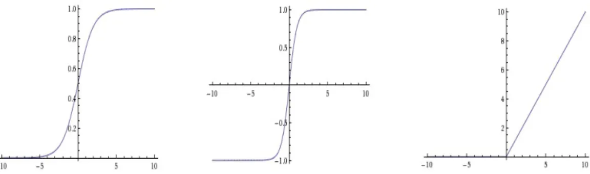
Figure 13: The left diagram is sigmoid, middle is tanh, and right is ReLU non-linearity (Li, 2018).
ReLU: Rectified linear unit computes the function f(x) = max(0, x). It means that the activations below zero are clipped to zero and the activations above zero remain same. The slope is 1 for the activations above zero. Alex et al. (2012) showed that ReLU accelerated convergence of stochastic gradient descent. It is very simple to calculate in comparison to sigmoid or tanh.
Feed-forward neural network
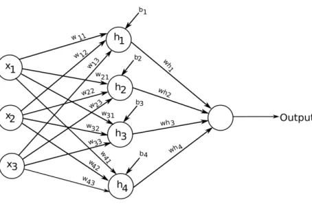
The individual neuron units are connected in a graph to form a neural network. The network is called feed-forward because the input flows towards the output in forward direction and there is no feedback from the forward branch to backward branch. A simple form of feed-forward neural network is shown in Figure2.5.
There are three layers in this network. The leftmost layer is called input layer. The middle layer is hidden layer which consists of neuron units and does the calculations. The rightmost layer is called output layer. The output layer is a single linear neuron here, depending upon the task in hand the output layer’s size changes.
Let us denote the input features by x which is a length mcolumn vector. The weights for the hidden layer and output layers are W1 and w2, respectively. The
Figure 14: A simple feed-forward neural network with one hidden layer.
biases for hidden layer neuron areb. The output of the feed-forward network can be given as below.
y=ϕ(W1x+b)w2, (14)
where ϕ is an activation function, x= [x1, x2, x3]⊺,
W1 = ⎡ ⎢ ⎢ ⎢ ⎣ w11 w12 w13 w21 w22 w23 w31 w32 w33 w41 w42 w43 ⎤ ⎥ ⎥ ⎥ ⎦ , b= [b1, b2, b3, b4]⊺, and w2 = [wh1, wh2, wh3, wh4]⊺.
In modern neural networks a large number of hidden layers are incorporated in a long chain. The output of a hidden layer becomes the input of next hidden layer. The overall length of the chain gives depth of the model. The deep term in deep learning comes from this deep chain of hidden layers. The number of hidden layers determine thedepth and the dimensionality of the hidden layer (number of units in a hidden layer) determines thewidth of the model (Goodfellow et al.,2016b: p. 164).
2.6
Overview of convolutional neural network
Most of the expansion of deep learning is the result of the success of convolutional neural networks (CNN). Although the use of CNNs goes back to 1998 (LeCun et al., 1998), their widespread use is due to much more recent event, when a deep CNN was
used by Alex et al. (2012) to beat a state-of-art level in the ImageNet classification challenge (Russakovsky et al., 2015). Since then, the development in computing power and the access to the large amount of data has brought CNNs at the forefront of rapid progression. For image classification tasks, many variants of CNN architec-tures have been successfully applied on ImageNet dataset namely VGG (Simonyan and Zisserman,2014), GoogLeNet (Szegedy et al., 2015), Resnet (He et al., 2016). However, the basic building blocks are very similar. The LeNet-5 (LeCun et al., 1998) is a simple and initial CNN architecture. LeNet network architecture is shown in Figure15. We will explain different processing layers in a typical convolutional neural network in following section.
Convolutional layer: Images can have millions of dimensions, and it is very
expen-Figure 15: LenNet-5 network (LeCun et al., 1998). The convolution of 6 filter kernels with the input image of 32×32 results in 6 feature maps of size 28×28 (C1).
In next layer S2, average pooling (subsampling) is performed using a 2×2 kernel.
Again a convolution (C3) and pooling (C5) was performed. Now the map values are
flattened and two fully connected layers (C5, F6) are attached. The output layer has 10 units for 10 classes.
sive to use fully connected layers. For example, if a 32×32 input is connected to a hidden layer of 1000 neurons, total number of parameters will be 32×32×1000 = 1.024 million, which is huge. Instead, convolutional layers come handy here. Convolution is a linear transformation which preserves the spatial properties of the images. The convolutional layer works as a feature extractor. When the filter weights are convolved with the input image, the output is called feature map. The weights of the filter are learned during the training. Several feature maps are obtained by using many different filter kernels. The idea is to extract important features like edges from the images. Moreover same filter weights can be used for the whole image, which reduces the number of parameters in the network and enhances the computations. Some kind of activation is also applied on the feature maps in order to give the model non-linear functionality. Thus a convolutional layer learns a set ofk filters g1, g2 ..,
k, 2D feature maps h, hk[x, y] = (f∗g)(x, y) = ∑ m ∑ n f[m, n]g[x−m, y−n] (15)
Figure 16: 2-D Convolution. f is a 2-D image which is convolved with the filter kernel g. The center pixel 5 showed inside the red box in the input image gets changed to -45 in the output imageh after convolutional operation.
Padding: In order to calculate the center pixel, it is important to consider the type of padding at the boundaries of the image. A common way is to add zero padding along the boundaries, so that the convolved output will be of the same size as of the input image. It is calledsame padding. In thevalid padding scheme in which we do not add any zero padding to the input, the size of the output would be reduced. Also, depending upon the type of strides and filter size used in the convolution, the output size of the feature map might change. Stride is the units by which the kernel moves left to right or up to down during convolution. The output width and height can be calculated using the following equations.
output width = w−fw + 2p sw + 1, (16) output height = h−fh+ 2p sh + 1, (17)
where w = input width, h = input height, fw = filter width, fh = filter height,
p= amount of zero padding, sw = horizontal strides, and sh = vertical strides.
Pooling: After the convolutional layers, the feature maps are down-sampled (or subsampled) using pooling. It reduces the spatial size of the features which in turn reduces the amount of parameters and the computations in the network. Pooling can be thought of as a summary statistic of the nearby outputs (Goodfellow et al.,
2016b: p. 330). One form is to apply a 2×2 kernel with a stride of 2 and taking the max value inside the filter box. This kind of max pooling (Zhou and Chellappa, 1988) is shown in Figure17.
Figure 17: Maxpooling.
Different filter sizes and strides are also used in the literature. Other forms of pooling can be seen as taking the average (shown as sub-sampling in Figure 15) or sometimes takingl2-norm (also known as euclidean norm or mean-square norm) of the elements inside the filter kernel instead of taking the max (Scherer et al., 2010; Rezaei et al., 2017).
Fully connected layers: The stacks of convolutional and pooling layers are followed by fully connected layers. In the fully connected layer, neurons are connected to all activations in the previous layer, as shown in the case of feed-forward network. Hence, the activations of the neurons are calculated by matrix multiplication followed by a bias offset.
Output layer: The output layer is generally a linear layer which takes the feature maps as input and transforms it into a score or probability. The length of output vector depends upon the number of classes.
Softmax is one type of output layer used in a multi class classification problem. For a given input, it outputs a probability of belonging to each of the class.
Training Process
The training data is usually divided into three sets, namely: training, validation, and test set. The model is trained with the training data and tested on the validation data during training. Once the training has converged, the trained model is tested on unseen test data. The training or learning process has three major steps.
Forward pass: The network takes an inputx and produces an output y. This is called forward propagation. Also, a scalar costL is calculated.
The neural network tries to find a function which maps input to a given output label. The learning of this function is done by providing set of input and output pairs, called training set. In practice, for supervised learning and classification problem, we have a set of inputs and corresponding labels. For example, the input can be a two dimensional matrix such as an m×n size image, that is, the input is a m×n
dimensional matrix. During the training, the network compares its output y to the real image label and tries to minimise the difference between the predicted output and real label. The idea is to maximise the likelihood of the prediction. In order to do so, the negative log likelihood (loss or cost) is minimised using some optimization tech-niques. The loss function can be formed depending upon the type of problem in hand. A typical form of loss function used in convolutional networks for classification tasks iscross entropy loss which is the cross entropy between the training data and the model’s predictions. The cross-entropy loss for a binary classification problem (class 0 and 1) is calculated as,
L=−(ylog(p) + (1−y) log(1−p)), (18) where y and p the correct class label and predicted probability by the model, re-spectively. The more general form of cross-entropy loss for multi-class problem is,
L=−
C ∑
i=1
yilog(pi), (19)
where C is number of classes, yi and pi are the correct class label and predicted
probability by the model for theith class, respectively.
Backward pass: In this step, the gradient of the cost function is calculated using back propagation. The partial derivatives of cost function L are calculated for all weights w and biasb. Since the information from the cost function flows backward in the network for gradient computation, this process is called back-propagation (Rumelhart et al., 1986a;LeCun et al., 1989) or back-prop.
Computing an analytical expression for the gradients of the cost function with respect to the network parameters is a computationally expensive task owing to the number of parameters in the neural net. Fortunately, we have a method called chain rule of derivatives to calculate the gradient of the scalar loss with respect to any parameter in the network. For more information reader can refer toNielsen(2018). Optimization: Optimization is the task of either minimizing or maximizing some function. Here we are interested in minimizing the loss function. Once all gradients are computed, network parameters are updated using an optimization technique. The loss function of CNN is highly non-convex and does not have a global minimum. In stochastic gradient descent(SGD) optimization, the loss is reduced by moving in small steps with the opposite sign of its derivative. The small step is calledlearning rate. Learning rate can be fixed or dynamic. The loss is calculated for each training
sample and the process is repeated iteratively until the algorithm seems to converge.
θ ←θ−ϵ∇θL(f(x;θ), y), (20)
where θ is the network parameter to be updated, ϵ is a scalar learning rate, and ∇θL(f(x;θ), y) is the derivative of the loss function L with respect to θ. It is
computationally costly and time taking to iterate over each training sample. In mini-batch SGD, the update is performed for every mini-batch ofn training samples. The algorithm has been found to converge faster by this method. It reduces the variance of the parameter updates, which can lead to more stable convergence.
θ ←θ−ϵ∇θ n ∑
i=1
L(f(xi;θ), yi). (21)
Adaptive moment estimation (Adam) optimizer (Kingma and Ba, 2014) com-putes adaptive learning rates for each parameter. It stores exponentially decaying average of past squared gradients vt and past gradients mt. The calculations are as
below,
mt=β1mt−1+ (1−β1)gt, (22)
vt=β2vt−1+ (1−β2)gt2, (23)
where mt and vt estimates first moment (mean) and second moment (variance) of
the gradientsgt respectively, and β1 and β2 are constants (close to 1). The authors
found that mt and vt are biased towards zero, the bias corrected first and second
order moment estimates are,
ˆ mt= mt 1−βt 1 , (24) ˆ vt= vt 1−βt 2 . (25)
Finally, the Adam update is:
θ ←θ− √ ϵ ˆ
vt+δ
ˆ
mt, (26)
where δ is a constant for stabilization in the case ˆvt becomes zero.
Regularization techniques
One of the focus of machine learning is to increase the generalization capability of the model, that is, in addition to the validation set, the model should perform equally well on the unseen data. Following are the major regularization techniques used in this work.
weight decay, which adds an additional term to the cost function to penalise parame-ters such that it drives weights closer to the origin. That means it penalises large increase in weights. The new cost function is,
J(x, y) = L(f(x;θ), y) +λ∑
i
θ2i, (27)
where λ∈[0,∞) is a hyperparameter that weights the contribution of regularization term.
Data augmentation: The best way to make a machine learning model gener-alise better is to give it more data (Goodfellow et al., 2016b: p. 233). In practice, the amount of training data is limited. One way to solve this problem up to a certain limit is to generate more fake but representative data. For images, many techniques like shift, rotation, contrast change, vertical, and horizontal inversion are some methods to augment the data as demonstrated byWang and Perez(2017). Dropout: Dropout (Srivastava et al., 2014) is a recent and simple but effective data regularization method. Dropout refers to dropping (ignoring) some of the neuronal units during the training phase. The set of neurons to be ignored is chosen randomly. At each training stage, individual unites are either dropped out of the network with probability 1−p or kept with probabilityp, so that a reduced network is left. It has been shown that dropout forces a neural network to learn more robust features and reduces the possibility of over-fitting in convolutional neural networks (Wu and Gu, 2015).
Transfer Learning
In machine learning, transfer learning is, applying models trained on one task on another task. For example, networks trained on ImageNet datasets are widely utilised in medical imaging applications (Shin et al., 2016). A machine learning algorithm trained for the classification of every day color images, such as cat and dogs, could be used to classify radio-graphs. The idea is that all images share similar features such as edges and blobs, which makes transfer learning feasible. In addition, deep neural networks often require large datasets (in the millions) for the proper training. Starting the training with weights from pre-trained networks might perform better than the random initialization if we have small dataset (Tajbakhsh et al., 2016; Zhou et al., 2017). In medical imaging classification tasks, the training data is often limited.
3
Materials and Methods
The experiments involved three major steps: data acquisition, model training, model testing. A number of deep learning frameworks are available to easily build neural networks from existing modules on a high level. Caffe (Jia et al., 2014), Theano (Theano Development Team,2016), TensorFlow (Abadi et al.,2016), PyTorch (Paszke et al.,2017) and Keras (Chollet, 2018) are some of the frameworks for implementing neural networks. We used Keras for our experiments as Keras comes with Theano and TensorFlow backend. It is easy to use and is continuously being maintained and updated. It runs seamlessly on CPU and GPU. It is very simple with emphasis on rapid model development. It has very good documentation containing many code examples and other resources that help users to get started very quickly. We also used CUDA (parallel computing platform and API model which enables graphics processing unit (GPU) for general purpose processing) and cuDNN (GPU-accelerated library of primitives for deep neural networks) for model development on GPUs.
We worked on two different types of artifacts and our approach deferred for both. We will describe material and methods for the two tasks separately.
3.1
Geometry artifacts
3.1.1 Data acquisitionThe images were acquired using six lab phantoms available at the R&D facility of Planmeca Oy using ProMax 3D Mid CBCT device. The data was acquired using a robotic automation script developed at Planmeca Oy. Canine Left and Canine Right sub-programs were used to acquire the training images. We acquired 9 volumes for the training, the size of each volume was 268×268×334. From each volume, 123 2D axial slices were taken and a total of 1107 images from 9 volumes were used for the training. The motion artifact was synthetically induced in the non-motion images by corrupting the geometry file. The number of motion images were same as the number of non-motion images. A total of 2214 image slices were available for training after taking the motion images into count.
Synthetic motion images: It was easier to produce large dataset of motion images from non-motion images by changing the geometry file and reconstructing the volume from the corrupted geometry file. We used three volumes of real motion images and their corresponding motion artifact corrected volumes to generate a function by fitting a normal distribution on the geometry file difference between motion and non-motion images. We induced motion artifacts in the images by adding randomly sampled values from the fitted function to the original geometry files of the non-motion images.
Figure 18: One of the phantom set up used to acquire the training data with Promax mid CBCT device (Courtsey of Planmeca Oy).
3.1.2 Image preparation
Image intensities were normalised from 0 to 1 for the whole 3-D volume by dividing each pixel by the maximum pixel value of the volume. This was the only preprocessing done on the images. Each image slice was divided into 60×60 resolution patches with 50% overlap (see Figure19). For simplification, it was assumed that all patches in the motion images contain motion artifacts. The total number of patches available were 141,696. The patches from non-motion images were assigned label 0 and the patches from the motion images were assigned label 1. 80% of the patches were used for the training and 20% patches were used for the validation.
3.1.3 Network architecture
We used a method described byKüstner et al.(2018) for the motion artifact detection in MRI images. The network used is called CNNArt by the authors. The network takes image patches as input and outputs the probabilities of belonging to class 0 (non-motion) and class 1 (motion), for each patch. Keras library (Chollet, 2018) was used for the network implementation with TensorFlow backend. Training was performed using two NVIDIA Geforce GTX-780 cards with 3 GB RAM each.
Below is an example of Keras sequential API to create network model. The model object is called using sequential API. Layers and activation can be added in series. Convolutional kernel coefficients were initialized by a Gaussian distributed
Figure 19: The left image is an input image of size 268×268 and the right image shows 64 patches of size 60×60 made from the left image with 50% overlap.
randomization. For the output predictions, a softmax layer is added in the last.
cnn = Sequential ()
cnn . add ( Conv2D (32 , kernel_size =(14 , 14) , kernel_initializer =’ he_normal ’,
weights = None , padding =’ valid ’, strides =(1 , 1) ,
W_regularizer = l2 (1e−6),input_shape =(60 ,60 , 1)))
cnn . add ( Activation (’ relu ’))
cnn . add ( Flatten ())
cnn . add ( Dense ( output_dim = 2, init = ’ normal ’, W_regularizer =’l2 ’))
cnn . add ( Activation (’ softmax ’))
Figure 20: The convolutional neural network with three hidden layers, one fully connected layer and one softmax layer as output. The size of input isH×W ×D, whereH is height, W is width and D is depth of the input. In our experiment, the input size is 60×60×1. The outputs of the network are the probabilities for the two classes, in our case, motion and non-motion (Küstner et al., 2018)
CNN filter coefficients were trained by optimizing the categorical cross-entropy loss function for a learning rate of 0.0001 with L2 coefficient regularization. The
cost function was optimized using Adam with corresponding parameters as β1 = 0.9, β2 = 0.999 and ϵ= 108 as used by the authors inKüstner et al. (2018) and described
byKingma and Ba (2014) in original Adam article as good default settings for the tested machine learning problems.
The below Keras code creates the optimizer object with custom parameters. opti = keras . optimizers . Adam ( lr =0.0001 , beta_1 =0.9 , beta_2 =0.999 ,
epsilon =1e−08, decay =0.0)
As shown in the below code, model training was run for 500 epochs and the model for the epoch with the lowest validation loss was saved using Keras call-backs object. In Keras, model needs to be compiled before the actual training starts, where the loss, optimizer, and metric (to be used for the training) are spec-ified. Finally the training was run using fit function. The training and validation datasets are given to the fit function as input. "batch_size" determines number of samples taken at a time and "verbose=1" prints the training progress on the screen.
iEpochs =500 batchSize =32
callbacks = keras . callbacks . ModelCheckpoint (’ model . h5 ’,
monitor =’ val_loss ’, verbose =1 , save_best_only = True ,
save_weights_only = False , mode =’ auto ’, period =1)
cnn .compile( loss =’ categorical_crossentropy ’, optimizer = opti , metrics =[’ accuracy ’])
result = cnn . fit ( X_train , y_train ,
validation_data =[ X_test , y_test ], nb_epoch = iEpochs ,
batch_size = batchSize , callbacks =[ callbacks ], verbose =1)
For the testing of the trained model, we used canine images from the 6th phantom,
which were not used for the training. Also, the performance of the model was tested against volumes from the other sub-programs like temporal bone and jaw. The test slices were first divided into the 60×60 patches and the softmax function gave probabilities for each patch of belonging to both motion and non-motion classes. We considered only the probability of motion class. Patches with probability of greater than 0.5 for motion class were taken as having motion artifacts. Finally, to get percentage of patches in a 2D image slice, below formula was used: