Sparse Solutions for Single Class SVMs: A Bi-Criterion Approach
Santanu Das
∗Nikunj C. Oza
†Abstract
In this paper we propose an innovative learning algorithm -a v-ari-ation of One-cl-assνSupport Vector Machines (SVMs) learning algorithm to produce sparser solutions with much reduced computational complexities. The proposed tech-nique returns an approximate solution, nearly as good as the solution set obtained by the classical approach, by mini-mizing the original risk function along with a regularization term. We introduce a bi-criterion optimization that helps guide the search towards the optimal set in much reduced time. The outcome of the proposed learning technique was compared with the benchmark one-class Support Vector ma-chines algorithm which more often leads to solutions with redundant support vectors. Through out the analysis, the problem size for both optimization routines was kept consis-tent. We have tested the proposed algorithm on a variety of data sources under different conditions to demonstrate the effectiveness. In all cases the proposed algorithm closely preserves the accuracy of standard one-class ν SVMs while reducing both training time and test time by several factors.
Keywords: Anomaly Detection, Optimization, Sparse, Scalability, Aeronautics
1 Introduction
Many problems in areas of interest to NASA, such as aviation safety and Earth science, have benefited and will continue to benefit from the use of data-driven methods for anomaly detection. For example, in avi-ation safety, many airlines have very large datasets rep-resenting the operation of their fleets of commercial air-craft. Most of this data represent normal operations of the aircraft—finding examples of anomalous opera-tion is comparable to the proverbial problem of finding a needle in a haystack. An algorithm to find anoma-lies in such a large dataset clearly needs to be fast and scalable. The algorithm also must be accurate, which requires leveraging as many properties of the dataset as possible. In particular, data from commercial air-craft contain continuous sequences, representing sensor data such as airspeed and altitude, as well as discrete ∗UARC, UCSC, NASA Ames Researchh Center, Moffett Field, CA 94035, [email protected].
†NASA Ames Researchh Center, Moffett Field, CA 94035, [email protected].
sequences, such as sequences of pilot switch presses. An algorithm that learns from such sequences will tend to outperform typical machine learning algorithms that as-sume that data collected at every instant in time is in-dependent from data collected at every other instant in time.
We addressed the accuracy issue in [7], where we devised a Multiple Kernel Learning (MKL) version of one-class SVMs containing one kernel over discrete se-quences and one kernel over continuous sese-quences. We chose one-class SVMs as the basis of our developments because of its strong performance as reported by other researchers, its guarantee of optimality given a partic-ular training set, and the flexibility of kernel methods to utilize a variety of different types of features both in single kernel and multiple kernel methods. In [7], we demonstrated our algorithm’s effectiveness at find-ing anomalies within commercial aircraft data. How-ever, the running time of one-class SVMs is higher than for other algorithms that we use because of the need to solve an optimization problem.
In this paper, we address the speed and scalability issue discussed above. We do this through a bi-criterion formulation of one-class SVM—that is, we add a crite-rion to the objective function that biases the algorithm toward a sparser solution, which we demonstrate theo-retically and experimentally. We show that our learning algorithm often has much lower training time than the classical one-class SVM learning algorithm. In some cases, our learning algorithm’s run time is higher, but we demonstrate that, in all these cases, our algorithm’s time to generate a classification (normal or anomalous) for a new data point is much lower. In spite of this, our algorithm’s performance is nearly the same as that of the classical one-class SVM in terms of how it clas-sifies new data. We achieved all these results without requiring any changes to the format of the data or any changes to the rest of the algorithm, such as the opti-mization problem solver, thereby making the algorithm easy to implement.
In the following section we provide some back-ground research to speed up and scale Support Vector Machines. This will be followed by our motivation and contributions. In Section 3, we describe the optimiza-tion problem of original one-class support vector
chines model which is the underlying algorithm of our work. Subsequently, Section 4 discusses the bi-criterion optimization which is the heart of this paper, followed by some details on the solver. Experimental evidence of performance of the proposed technique is given in Sec-tion 5. Finally we conclude the paper with a discussion in Section 6.
2 Background and Motivation
Kernel based methods like one-class support vector ma-chines have a significant disadvantage in addressing scal-ability to large number of training points. With increas-ing trainincreas-ing points, the trainincreas-ing time and the memory requirements drastically increase and at the same time the prediction time which is proportional to the number of representative support vectors also increases. The number of representative support vectors also holds a proportional relationship with the number of training points. There have been several efforts to over come training and testing time scaling issues either by build-ing an online algorithm, a parallel batch algorithm, or a sophisticated scheme to select more informative training samples. A lot of researchers reported satis-factory contributions in multiple areas like data pre-processing, data compression, kernel modification [12] etc., while others have investigated more in the areas of optimization and solver development. Each of these tasks individually plays an important role in building the model. In [3] Burges and Sch¨olkopf proposed “re-duced set” method in order to improve on classifica-tion speed and “virtual support vectors” method to im-prove on accuracy, however at the cost of some increased training time. Some papers talk about how to improve the performance of kernel based methods in general. Most of these literatures examine techniques for effi-cient matrix factorization, low rank approximation, etc. Schwaighofer and Tresp [17] conducted a comprehensive study on using some of these approaches to scale Gaus-sian process regression technique on large data sets. Asharaf et al. addresses the scalability problem of SVMs using cluster based training [1, 14] where some selected samples representing the cluster abstractions of the en-tire training data are used to build the model without compromising the generalized performance. However the outcome of cluster based training will typically de-pend on the performance of the clustering algorithm. Liang Lie-quan and Liang Ying-hong [11] used a mode sensitive procedure called “mean shift” algorithm for clustering purpose. Another popular technique is chuck-ing algorithms [18] which solves a smaller QP problem formed by samples corresponding to nonzero Lagrange multipliers. A vast amount of papers discuss iterative training of support vector machines (e.g. [19, 5]). There
are separate examples of on-going research [13, 15, 8] looking for effective and efficient solvers that can han-dle large data sets and improve scalability of machine learning methods which may require solving optimiza-tion problems.
The scope of our current effort is intentionally restricted to scaling up the batch version of classical one-class SVMs formulation [16] without having to change the optimization problem solver. We assume that the entire data set can fit into memory but we plan to extend our algorithm in the future to run online or in parallel. Moreover we pose the additional restriction of not training or building the model iteratively to reach certain objective [6].
The work most closely related to this one is the “simple decomposition method” idea presented in [20]. The key idea in [20] is to avoid the burden of general linear constraints from the optimization and convert
it to a simple bound-constrained problem. In our
formulation we do not get rid of any linear constraints. Instead we take advantage of the relationship between the set of linear constraints and the bound information of the design variables. To the best of our knowledge, none of the existing literature discusses formulating this non-trivial regularized approximation from prior knowledge of constraints in the optimization problem
that leads to a sparse one-class SVMs. Our main
contributions in this paper are:
• We propose an optimization problem with an
addi-tional meaningful criterion. The proposed formula-tion is acceptable and still equivalent to the classi-cal SVM problem in terms of generalization error. The proposed formulation is very simple and can easily be implemented.
• We provide reasoning on why the proposed
algo-rithm produces sparser solutions which in return improves the testing time by several factors.
• The proposed algorithm is several orders of
mag-nitude faster than existing learning method and at the same time it retains the accuracy of the bench-mark algorithm. We provide theoretical explana-tions for this.
• We demonstrate the capability of the algorithm in handling simulated data sets with varying sparsity and real life data from airlines industry by mea-suring the performance of the proposed technique using different metrics, such as frequency, accuracy, sensitivity, ranking,and run time.
• We provide some useful insights regarding the
effectiveness of proposed technique based on the experimental and simulation study.
3 Preliminaries on Single Class Support Vector Machines Origin Marginal SVs Non−SVs Non−marginal SVs hyperplane Seperating w kwk ξi ρ kwk
Figure 1: This figure illustrates the geometric interpre-tation of optimal hyperplane for one class Support Vec-tor Machines.The empty circles, solid circles and the dotted circles represent non-support vectors, bounded support vectors and unbounded support vectors respec-tively.
Sch¨olkopf [16] introduced one-class SVMs as an
unique member of the SVMs family. As the name
suggests, one-class SVMs is a unsupervised learning method which is trained on a single class and used for estimating the density of the target support objects. In standard one-class SVMs problem, we are given a set of labeled training data D={(~xi, yi)}ni=1 in the input
space R, where ~xi ∈ Rd and the corresponding labels yi ∈ {+1}. The key idea is to construct a hyperplane
that can separate outliers from the rest of the training examples, as shown in Fig. 1. At the end, we wish to develop a decision rule from the seen samples, so that when a new point comes in, we will be able to assign a class level depending on whether the model has seen this point or not. Since aN−1 dimensional hyperplane can exist in the N-dimensional feature space, the primary task is to find the optimal separating hyperplane that can maximize the margin between the training examples and the origin, which is the lone representative of the second class with negative label. This can be achieved by solving an optimization problem that leads to a set of training points, termed “Support Vectors” (SVs) which are the representatives of the decision boundary.
Let us define a function φ that can be used to
map variables from the input space to the feature
space F, i.e. φ : Rd → F. In feature space the
inner product hxi,xji property holds, where xi := φ(xi). While evaluating the dot product in the feature
space, the explicit calculation using mapped feature
φ can be avoided by simply evaluating the kernel
function i.e. k(xi, xj) := hφ(xi), φ(xj)i. However
in order to do so, the chosen inner-product kernel
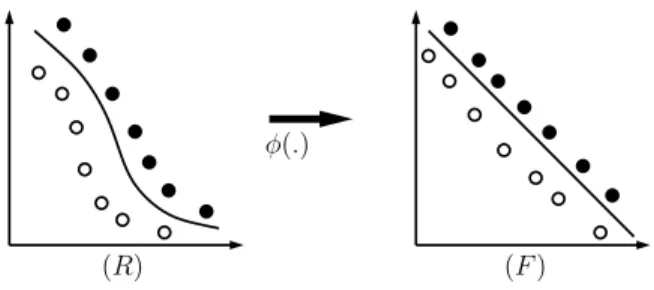
(R) (F)
φ(.)
Figure 2: In this figure we provide the illustration of higher dimensional mapping for linear separation fields. It shows that even if the patterns are nonlinearly separable in input space, it is possible to map them in higher dimensional feature space where they may be linearly separable. Here φ(.) is the mapping function.
must satisfy Mercer’s theorem [4]. We will see an
example of a normalized Longest Common Subsequence (nLCS) based kernel function later where we discuss our experimental studies.
3.1 Derivation of the Optimization Problem:
In order to construct the optimal hyperplane we solve the following primal problem (Eqn. 3.1). The expres-sion in Eqn. 3.1 simply means, “maximize the margin between the origin and the hyperplane (Fig. 1) for a nonseparable problem [16] in the feature space”. The primal problem is represented as
minimize P(w, ρ, ξi) = 1 2ww T + 1 νℓ ℓ X i=1 ξi−ρ subject to (w.φ(xi))≥ρ−ξi, ξi≥0, ν∈[0,1] (3.1)
where ν is an user specified parameter that defines the upper bound on the training error, and also the lower bound on the fraction of training examples which are support vectors, ξ is the non-zero slack variable, ρ is the offset, φ(xi) represents the transformed image of xi in the Euclidean space andi ∈[ℓ]. The position of
the optimal margin relative to the origin is represented byρ, which in fact is the margin of separation between positive and negative class.
Using Lagrangian and some simple manipulations, the constrained primal problem (Eqn. 3.1) is converted to a dual problem [4],
minimize Q= 1 2 X i,j αiαjk(xi, xj) subject to 0≤αi≤ 1 νℓ,1− X i αi= 0, ν ∈[0,1] (3.2)
It is not difficult to show that ρ =P
iαik(xi, xj)
for the solution w and pattern xi corresponding to
0< αi<1 while settingξi= 0.
Weights to training points are Lagrangian multipli-ers (α~) that ranges between 0 and 1. There exist at least
νℓ non-zero Lagrangian multipliers. Support Vectors
(SVs) are training points{xi:i∈[ℓ], αi>0}with
non-zero weights. Non-margin or bounded SVs are the ones with{xi:i∈[ℓ], αi= 1}and margin or unbounded SVs
are those with{xi :i∈[ℓ],0< αi<1}.
Once ~α is known, SVMs compute the decision
function, f(x~j) =sign( X i∈Im αik(~xi, ~xj) + X i∈Inm k(~xi, ~xj)−ρ) (3.3) where I0={i : αi = 0}, Im={i : 0< αi <1}
and Inm = {i : αi = 1} are the sets of indices
of Lagrangian multipliers corresponding to non-SVs, marginal and non-marginal support vectors respectively. The pseudo-code of one-class SVMs algorithm is shown in Algorithm 1. Given a test pointxj, iff(x~j)<0, then xj is predicted to be an outlier, whereas if f(x~j) ≥0,
thenxj is predicted to be normal.
Algorithm 1Single Class SVMs Algorithm 1: Input Vector: X={x1, x2....xm, z},X∈ Rd.
2: Map Features: K(φ(xi), φ(xj))).
3: Solve Eqn. 3.2 to obtainαcorresponding to Support Vectors (SVs). 4: Calculate bias,ρ=PNsk=1αkK(Φ(~x)Φ(x~k)). 5: Calculate score,f(~z) =PNsk=1αkK(Φ(x~k)Φ(~z)). 6: if f(~z)> ρthen 7: return 1 8: else 9: return 0 10: end if
4 The Multi-criterion Optimization
The multi-criterion optimization problem has several fascinating applications that compromise Economics,
Engineering, Mathematics etc. Given a set of criteria q(x) =P
iλifi(x) and a set of feasible points Ω∈Rn,
the key idea is to find the optimal point x ∈ Ω, for
whichq(x)≤q(z),∀zfrom the feasible set. This can be expressed as, min x∈Rn q(x) subjected to ci= 0, i∈ε ci≥0, i∈I (4.4)
where ci = 0,i∈εare equality constraints andci ≥0, i∈Iare inequality constraints. There are methods [10] that also find multiple solutions that cover the full set of possible trade-offs between the various objective func-tions. The selection of these criteria are typically based on the knowledge of optimal design or control variables, summary statistical, model assumptions, target objec-tives like smoothing, de-noising etc. A detailed descrip-tion of techniques that take care of the trade-off between multiple criteria can be obtained in [2].
4.0.1 Bi-criterion Formulation: The Main Idea
To make the dual formulation more effective, we take into account the structure of the linear constraints and their dependencies on the variable bounds. We do this approximation by incorporating a second-order penalty function, keeping in mind the description of support vectors and the properties of the associated Lagrangian
multipliers/weights. The bi-criterion formulation of
one-class SVM takes the form of,
minα∈ℜn Q= 1 2α TKα−λ( 1 2νℓ~1−α) T( 1 2νℓ~1−α) subject to 0≤α≤ 1 νℓ~1,~1 Tα= 1, ν∈[0,1] (4.5)
whereαis the vector of Lagrangian multipliers and
K is the similarity matrix. The motivation behind
the additional penalty term is that the bi-criterion formulation seeks the values of the design variables closest to the extreme (upper or lower) bounds of the design variable while simultaneously minimizing the
first term. Only training points with non-negative
weights are considered as support vectors. It is very intuitive that the equality constraints are satisfied with the least number of design variables only when the weights corresponding to those variables tend to be close to the maximum possible value (i.e. αi = νℓ1). Hence
by solving the above problem we expect to obtain a sparse solution. In the following sections we will see that the quadratic penalty function is compatible with the method of direction search and plays a significant role to reach the optimal solution using less computations.
Proposition 4.1. Bi-criterion formulation (Eqn. 4.5) of SVMs is convex.
Proof. Solving this optimization problem means that we
need to minimize two convex criterion on a defined set:
• The Hessian of the objective function Q(in Eqn.
3.2) of classical One-class SVMs problem is given by ∇2
xQ(x) = K, where K ∈ Sn+ is a symmetric
kernel matrix. Since we make sure that the defined kernel matrix is positive definite or positive semi-definite, it implies that the objective function is either strictly convex or convex.
• Since the controlled criterion takes the form of a squared Euclidean normh= ( 1
2νℓ~1−α) T( 1
2νℓ~1−α), his strictly convex.
• Given 0 ≤ αi ≤ νℓ1, the constraint in Eqn. 3.2
defines convex set asP
iαi is convex.
Here we will briefly discuss the nature of solutions
that bi-criterion formulation may yield. With the
control parameter λ = 0 (Eqn. 4.5), we would get
the classical solution. However with a non-zero control
parameter, (say λ = 1), the quadratic term leads to
sparser solutions. Suppose we are given ℓ training
samples and model parameter ν ∈ [0,1], and define
p = νℓ. The upper bound of the constraint (Eqn.
3.2) is 1
p. The second order term of the objective
function attains its maxima at 0 and 1
p and therefore,
the solution will tend to push theα’s toward the extreme
values in the range. Since P
iαi = 1 and αi can
attend a maximum value of 1
p, we can, without the
loss of generality, decompose the previous expression as,
PN i=1αi = Pp i=1αi+ PN i=p+1αi =p 1 p+ 0 = 1. Hence
the solution is a set ofptraining inputs with maximum weights i.e,α1=α2=α3=· · ·=αp=1p. Ifpis not an
integer, it is rounded to the nearest integer value (say ˆp) and the above process is repeated. This results in ˆp−1 design variables attaining the upper bound and thus forcing the remaining ones to take any values from the range defined by 0≤αi ≤ 1p such thatPiα
ˆ
p
i=1 = 1 is
satisfied. Therefore with aλwhich is large enough, the optimization is pushed toward a solution that is more sparse than the classical solution.
4.1 Active Set: The Quadratic solver “Active set” algorithm [9, 15] is very popular in solving QP problems with constraints, especially when the positive semi-definite matrixKis dense in nature. Equation 4.5 can be rewritten as,
minα∈ℜn Q= 1 2α TKαˆ +CTα subject to 0≤α≤ 1 νℓ~e, ~e Tα=b, ν∈[0,1] (4.6) where ~e = ~1, b = 1, ˆK = K −2λI, C = λ νℓ~e.
The optimization problem defined above is a quadratic programming problem with a linear set of constraints and we would like to solve this problem in a finite number of steps using “Active set” algorithm. In active set algorithm, the first step is to compute a feasible start point which satisfies both the bounds and the equality constraints. Given a feasible start point α0, the task is
to iteratively minimize the objective function. However this requires us to find the suitable direction of search and a non-negative step size.
Definition At any α, the active set A(α) consists of free variable indices from the equality constraints to-gether with the indices of variables which are temporar-ily fixed on their upper/lower bounds.
4.1.1 Reduction of Problem Size At any kth
it-eration, suppose we have some αk. We would like to
create a partitioning of the active set. If “X” refer to en-tities corresponding to design variables whose values are temporarily fixed and the complement set of variables, termed as free variables, are denoted by “R”, we can cre-ate a partitioning of current pointsαk i.e. αk= [αRkαXk]
andn= [nXnR] wherenis the cardinality of the design
variable. Similarly we can also define the partitions is A= [ARAX] andC= [CRCX]. We can also define,
ˆ K= ˆ KR,R KˆR,X ˆ KX,R KˆX,X .
where ˆKX,R = ( ˆKR,X)T. At iteration k, we can
define a working set Wk which is constructed by t
equality constraints only. Temporarily discard all the
fixed variables so that we end up with n = nR and
t = mℓ, whereℓ denotes the total number of equality
constraints. The direction of search is computed by solving the following reduced problem,
min α∈RnQ= 1 2αk RTKˆR,RαR k +CRTαRk subjected to 0≤αR k ≤ 1 νℓ~e, A RTαR k =b −AX TαX k, ν∈[0,1] (4.7)
Once the reduced problem is formed, the next task is to check ifQ(αR) is minimized for the given αR
Wk. If Q(αkR) is not minimized, we need to compute
the direction and the step size such that Q(αk+1R) ≤
Q(αkR). The pseudo code of the algorithm to compute
the direction and the step size is shown in Algorithm 2. The bi-criterion formulation tends to push the α’s toward the extreme values in the range. However the optmization prefersαi to attend the maximum value of
1
p to maintain a finite step size in the suitable direction.
As a consequence, the number of bounded variables quickly increases, thus resulting in a much smaller problem (Eqn. 4.7) to solve. The reduced QP problem (step-3, Algorithm 2) can be solved using elimination of variables or Lagrangian Methods.
Algorithm 2Sub-problem of active set algorithm 1: Input: αkR,KˆR,R, CR. Let direction is denoted by
dkR=αk+1R−αkRandgk=αkRTKˆR,R+CR. 2: Q(αk+1R) =Q(αkR+dkR) = 12(αk R+ dkR)TKˆR,R(αkR+dRk) +CRT(αkR+dRk) = Q(αkR) +12dk RTKˆR,Rd kR+gkTdkR. 3: Modified sub-problem mind 12dk RTKˆR,Rd kR+gkTdkR subjected to,ARTd kR= 0 4: if dkR6= 0 then
5: Calculating step size along the directiondkR
6: if αkR+dkR is feasiblethen
7: setαk+1R=dkR+αkR
8: else
9: setαk+1R=γkdkR+αkR, step sizeγk∈[0,1]
10: end if 11: else
12: Check for KKT condition" ˆ KR,R AR ART 0 # dkR −θ = − αkRTKˆR,R+CR 0 13: end if
5 Experiments and Discussions
In this section we conduct computational experiments of bi-criterion SVMs and present some studies compar-ing bi-criterion and classical SVMs. In our analysis, we considered two very different data sets: one real-world FOQA (Flight Operations Quality Assurance) data and another simulated data set as benchmark applications. The aviation data is representative of one of the most complex engineering systems with very large size and dimensionality. Such a domain also poses a real chal-lenge in identifying anomalies in high-dimensional,
mul-tivariate data sets containing discrete, categorical, and continuous features. Therefore it is an ideal platform to test the accuracy and scalability of anomaly detection algorithms. The simulation based study was proposed to conduct a proof- of-concept analysis that demon-strates the performance and effectiveness of the pro-posed bi-criterion algorithm under different test con-ditions. Both bi-criterion and classical one class SVMs algorithms were tested on Linux cluster that comprised of 16 slave nodes, each of which is a dual processor 1−U server containing two, quad-core Intel Xeon pro-cessors @ 2.66GHz totaling 128 cores and 128GB Ram (1Gb/Core). It is controlled by two master nodes and has 30T b storage. Under each test condition, the de-sign variable of the optimization from bi-criterion and classical one class SVMs were initialized with the same random set to preserve consistency.
5.1 Airlines Data: A Realistic Scenario The real world data set chosen for analysis is from a com-mercial airlines. The data is obtained from medium range narrow body passenger aircraft. In our current analysis we considered a total of 2048 flights, a small subset of which landed at the same airport. Each flight consists of 365 parameters acquired at 1 Hz. Our work-ing data set consists of the decent portions of the flight from 10,000 ft to touch-down (average flight length of
10K samples) and has 104 discrete and 45 continuous
parameters which were selected based on domain ex-perts feedback. For continuous data, each parameter in the training and testing data are z-score normalized using the statistics of each parameter calculated across all training flights. The continuous and discrete data is converted to continuous and discrete sequences respec-tively. Once the sequences are generated the continuous and discrete kernel are separately computed pairwise across all possible flight combinations in the training set. For pairwise comparison we used longest common subsequence based similarity function (Eqn. 5.8). (5.8) K(~xi, ~xj) =
|LCS(~xi, ~xj)| p
l~xil~xj ,
where l~x is the number of symbols in sequence
~x. Given two sequences the common subsequences of
sequences ~xi and ~xj is identified. The longest such
subsequence of~xi and~xj is called the longest common
subsequence (LCS) and is denoted by LCS(~xi, ~xj) and |LCS(~xi, ~xj)|is its length.
Once the kernels are generated, we combine them in a convex fashion. Algorithm 3 shows the operations to generate the kernel. For details see the original paper [7] where we demonstrated Multiple Kernel Anomaly De-tection Algorithm (MKAD) algorithm that can detect if
the discrete pilot inputs combined with the observation vector are nominal or off nominal.
Algorithm 3Pre-processing steps to generate a kernel 1: Continuous Input : C={x1c, x2c....xmc, zc},
C∈ Rd, Discrete Sequence Input :
S={x1s, x2s....xms, zs},S∈ Rde.
2: Generate Continuous Sequence:
{x1q, x2q....xmq, zq}=
SAX({x1c, x2c....xmc, zc}) [?].
3: Generate Continuous and Discrete Features:
{φ(x1q), φ(x2q),· · ·φ(xmq), φ(zq)}and {φ(x1s), φ(x2s),· · ·φ(xms), φ(zs)}.
4: Combine kernel:
βqKq(φ(xiq), φ(xjq)) +βsKs(φ(xis), φ(xjs)).
Active-set algorithm has been used to solve the quadratic problem. Through out this experiment, some of the user defined inputs for example, kernel matrix, initialization vector,νparameter, stopping criteria, etc., were kept consistent for both the algorithms. From run to run, the design variables were randomly initialized with values between 0 and 1. However for any particular run both the algorithm started from the same initial point. In the first set of experiments, both models were built with training sizes varying from 200 samples up
to 2000 sample points with ν = 0.05 and the number
of support vectors were recorded for each case. These results are unique and reproducible for the given data
and parameter settings. Figure 3 shows that
bi-criterion SVMs always produces fewer support vectors than the classical approach for different training sizes and the reduced set size is typically the lower bound of the number of total support vectors i.e. ν times the number of the training points.
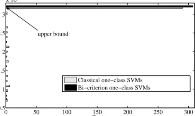
Figure 4 compares the distribution of the weights (αi fori∈[l]) corresponding to the support vectors for
a case where we used 2000 sample points for training and set ν = 0.05. For classical SVMs there are more instances where weights are scattered in-between the bounds. However for bi-criterion formulation we see all weights lie on the upper bound. Fig. 3 and Fig. 4 complement each other and show that our algorithm produces fewer support vectors by forcing weights to-ward the upper and lower bounds. In summary, with majority of the Lagrangian multipliers/weights on the upper bound, the model results in a much reduced set of non-zero weights.
Here we extend our observation from Fig. 3. We have seen that bi-criterion SVMs results sparser solu-tion when compared to classical model. The analysis (Fig. 4) showed that classical solution consists of 331
200 600 1000 1200 1400 1600 1800 2000 0 20 40 60 80 100 120 140 160 180 Number of observations
No. of support vectors
Classical one−class SVMs Bi−criterion one−class SVMs
Figure 3: Figure comparing the number of support vectors obtained from the bi-criterion and classical SVMs technique for different training sizes over a single run. For each and every run, bi-criterion formulation converges with a sparser solution and thus outperformed classical SVMs formulation. 0 50 100 150 200 250 300 0.5 1 1.5 2 2.5 3 x 10⁻³ Lagrangian multipliers/weights of SVs Counts Classical one−class SVMs Bi−criterion one−class SVMs upper bound
Figure 4: In this figure we compare the distribution of the weights of support vectors obtained from the clas-sical and bi-criterion SVMs. We can observe that most design variables in bi-criterion formulation corresponds to the “upper bound” (i.e. 1
νℓ, see Eqn. 3.2). For
clas-sical SVMs there are some instances where the design variables hold values between upper and lower bounds.
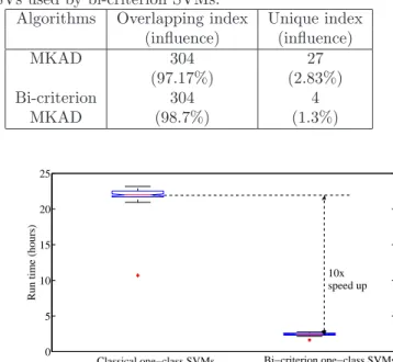
non-zeros weights while bi-criterion SVMs produced 308 which is exactlyν×2048, the number of training sam-ples. An initial investigation found that solutions from both these methods have a total of 304 support vectors in common and that jointly compromises approximately 97−98% of the total weights (see the linear constraint in Eqn. 3.2) which is unity. To account for the remaining weight, bi-criterion SVMs proposes 4 unique SVs while the classical assigns 27 SVs which can very well be some source of redundancy. These results are summaries in table 1.
Table 1: Here we compare classical and bi-criterion SVMs to check the presence and the influence of redun-dancy. The analysis showed that 304 indices (of Sup-port Vectors) are common in both solutions and they jointly compromises approximately 97−98% of the total weights. To account for the remaining weight, classical SVMs uses approximately 7 times the number of unique SVs used by bi-criterion SVMs.
Algorithms Overlapping index Unique index
(influence) (influence) MKAD 304 27 (97.17%) (2.83%) Bi-criterion 304 4 MKAD (98.7%) (1.3%) 0 5 10 15 20 25 QP QP with regularization
Run time (hours)
10x speed up
Classical one−class SVMs Bi−criterion one−class SVMs
Figure 5: The figure shows the run time analysis for classical and bi-criterion SVMs under different initial-ization conditions. This experiment was repeated 100 times with random initializations and the running time were recorded. These are observed run times with ran-dom initializations. It is clear that bi-criterion formula-tion performs much better compared to classical SVMs.
In Fig. 5 we show the resulting training time (in hours) for the exact solution and bi-criterion formu-lation with 2000 sample points as training points and ν = 0.15. In the box plot, we show the mean training time over 100 runs and their corresponding error bars. The mean rum times are 21.64 hours and 2.43 hours for classical and bi-criterion SVMs respectively. The stan-dard deviations are 2.4 and 0.23 for the respective mod-els. It can be observed that the proposed formulations consistently performs on average 10 times faster than the classical one-class SVM model for the given model parameter settings. This performance gain factor is ex-pected to increase with increasing training set size. In a separate experiment, we repeated the same case with randomly initializations from the feasible region defined
by the bound constraints. This led us to further gain in run time. This is because the optimization routine does not spend any time looking for a initialization set from the feasible region. However this observation is true for both the algorithms.
10−2 10−1 100
123456789 10 11 12 13 14 15 16 17 18 19 20 21 22 23 24 25 26 27 28 29 30 31 32 33 34 35 36 37 38 39 40 41 42 43 44 45 46 47 48 49 50
Sorted index of the top 50 anomalous in training observations
Normalized scores
(in log scale)
Bi−criterion one−class SVMs
Classical one−class SVMs
Figure 6: Normalized scores of the top 50 abnormal entries detected in the FOQA training set data. Both the scores were arranged in a descending order of the classical algorithm’s score. This experiment was repeated 100 times with random initializations. This figure shows that the bi-criterion algorithm almost always orders data points the same way as the classical algorithm.
In this section we present some results on prediction performance. In this analysis, we asked both the models to predict the top 50 outliers from the training pool of 2048 and we compare their associated outlier scores
and ranking. We sorted the outliers and thereafter
normalized them to 1. In Fig. 6 we compare the mean score with associated error bars from multiple runs in log scale. This experiment was repeated 100 times with random initializations. Figure 6 clearly shows that bi-criterion SVMs correctly predicts and ranks the points in terms of their outlierness in a consistent fashion and the outcome is very comparable to observations from classical one-class SVMs.
We have conducted an initial study that describes the nature of the solution we obtain for varying λ. In the bi-criterion formulation, the value of the λdecides
which criterion is weighted more. In Fig. 7, we plot
the number of support vectors for a wide range of λ
values. The case when we obtain maximum number
of support vectors is for λ = 0 and we normalize the
entire outcome using the maximum count. What we observed is, the number of support vectors drastically
changes ( 7% change) as we start increasing λ from
0 but as λ becomes large enough (greater than 0.5)
0 0.5 1 1.5 2 2.5 3 3.5 4 4.5 5 0.92 0.93 0.94 0.95 0.96 0.97 0.98 0.99 1
Weights of control parameter
Normalized parameter
(number of support vectors)
Figure 7: Figure demonstrating the influence of the
control parameter λ on the performance of the
bi-criterion SVMs algorithm. There is very small influence of the control parameter (λ) on the multi-criterion optimization outcome forλ≥ 1
2.
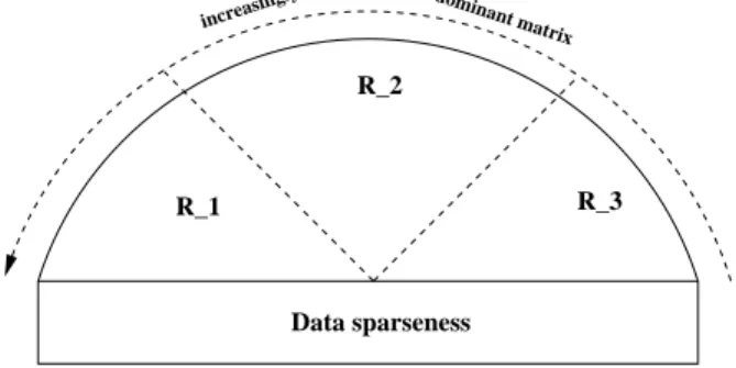
sparsity of the solution is steady for the given data and parameter settings. We therefore setλ= 1 for all of our experiments.. Data sparseness R_1 R_2 R_3 dominant matrix diagonaly increasingly
Figure 8: A cartoon that represents various levels of sparseness that can be observed in the kernel matrix K(xi, xj). Region-1 (R1) and Region-3 (R3) represent
extreme scenarios. When all entries of x and y are
very different from each other and unique, the resultant similarity matrix is strictly diagonally dominant (R1).
With very similar x and y the K matrix will be
very dense with very similar diagonal and off-diagonal elements (R3). Region-2 (R2) represents a case when
the diagonal and off-diagonal elements are distributed over a certain range.
5.2 A Simulated Study: To test the robustness of the bi-criterion formulation, we developed a common test platform with a set of diverse test scenarios using synthetic data. Till now we have studied the influence
of the quadratic penalty function (Eqn. 4.5) and the
control parameter on the outcome. For problems of this nature, the property of the kernel matrix (K) in Eqn. 4.5 plays an important role. The implicit mapping into feature space based on different similarity functions and data sets are bound to conceal different types of density structures in the kernel matrix. The main optimization algorithm involves quadratic programming which learns on these kernel matrices. Here we intend to investigate the influence of varying kernel density on model per-formance and outcome. When the entries of the input data xi and xj are very different from each other and
unique, the resultant similarity matrix is strictly diag-onally dominant i.e. |K(xi, xi)|>Pi=6 j|K(xi, xj)|,∀i.
The other extreme scenario is when all the entries x
andy are very similar in feature space and tightly clus-tered. The latter will result in a highly dense K ma-trix. In Fig. 8, we explain the above scenarios in a cartoon form. Region 1 (R1) and Region 3 (R3)
rep-resent the extremely sparse and highly dense cases, re-spectively. Region-2 (R2) represents a case when the
diagonal and off-diagonal elements are distributed over a certain range.
We will further illustrate the above scenarios of varying sparseness by using synthetic data set. This data is randomly generated from the normal
distribu-tion with user defined mean parameterµand standard
deviation parameter σ. The resultant kernel matrices we generate are symmetric and of size 2048. We force the diagonal elements to unity, as this is case for most similarity functions (e.g. nLCS function shown in Eqn.
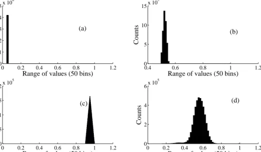
??) which vary between 0 and 1, where 1 represents the highest similarity or exact match. For each combination ofµandσ, we binned the elements ofKinto 50 equally spaced groups each of which represents a “values range” between 0 and 1. In returns we obtain the number of elements in each group. In the analysis, we conducted a total of 20 different cases where the density distribution of the matrix moves from one end of the “values range” to the other end. Figure 9 presents some of these exam-ples. Subfigure ??-(a) shows an example where all the elements of the kernel matrix, beside the diagonals, are of extremely small. This is a typical example of diag-onally dominant matrix. Subfigure ??-(c) is the other extreme case with very comparable diagonal and off-diagonal elements. Subfigure ??-(b) and Subfigure ?? -(d) represent a simulated and a realistic (aviation data) scenario where the off-diagonal elements of the matrix
K hold values from intermediate ranges. Under each
test condition, we ran 10 experiments with random ini-tializations and recorded the run time and number of support vectors for bi-criterion and Classical SVMs al-gorithm. To measure the effectiveness of the model, we
0 0.2 0.4 0.6 0.8 1 1.2 0 1 2 3 4 5x 10 6
Range of values (50 bins)
Counts 0.4 0.6 0.8 1 1.2 0 5 10 15x 10 5
Range of values (50 bins)
Counts 0 0.2 0.4 0.6 0.8 1 1.2 0 0.5 1 1.5 2x 10 5
Range of values (50 bins)
Counts 0 0.2 0.4 0.6 0.8 1 1.2 0 2 4 6x 10 5
Range of values (50 bins)
Counts
(a)
(c)
(b)
(d)
Figure 9: The above figure represents the histogram plots comparing the distributions of the elements of the kernel K under different test cases. Each element of K represents the similarity between two entities. The diagonal elements represent self similarities. Subfigure (a-c) was obtained from simulated data while subfigure (d) was obtained from a real airlines FOQA data consisting of 2048 flights with 149 continuous and discrete features. In subfigure (a) the kernel K is a diagonally dominant matrix while subfigure (c) represents the case where the diagonal and off-diagonal elements of the matrixKare very comparable. Subfigure (b) represents an intermediate scenario.
define the following two performance metrics.
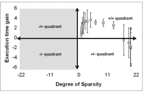
Definition We defined degree of sparsity, a gain met-ric, that calculates the ratio of the counts of non-zero Lagrangian multipliers from bi-criterion to that of clas-sical SVMs model. This metric explain how effective is the proposed model in testing phase. If degree of sparsity if high this simply implies that the solution is obtained with lesser support vectors.
Definition The execution time gain is a run time re-lated gain metric, that calculates the ratio of the run time of bi-criterion to that of classical SVMs model. This metric shows how quick is the proposed optimiza-tion converges to a soluoptimiza-tion compared to the benchmark method.
Figure 10 summarizes the results using the perfor-mance metrics in a quadrant format for a better vi-sual understanding. The two right hand quadrants al-ways confirm a sparse solution. Similarly the upper two quadrants indicates seep up by some factors. Anywhere
in the +/+ve quadrant is the most desired
operat-ing region where under any circumstances the proposed solution is sparse and the execution time is less. A neg-ative execution gain means that the classical solution
converges faster. In Fig. 10, the execution time gain is intentionally plotted in log scale to obtain a better resolution in order to understand the differences in the performance space. As can be seen, bi-criterion formu-lation outperforms the benchmark algorithm consider-ably in most cases. On all occasions, bi-criterion SVMs always reported the lest number of support vectors (i.e. νN) but the solution of the classical method changes depending on the density structure of the kernel ma-trix. For instance, from diagonally dominant matrix (refer Fig. 8 region -1 and Fig. 9 -(a)) classical SVMs
reports N support vectors which is equal to the
num-ber of training points. This is because all the training examples are so different and unique that all of them carries equal weightage to be a support vectors. How-ever the convergence time of the classical approach was varying a lot. Under this scenario, there were several occasions where bi-criterion ran slower than the classi-cal SVMs by a couple of factors. But majority of the gain was noticed during test phase where to evaluate a single test point the classical will have to do at least 1
ν
times more operations. On the other hand for highly dense kernel matrix with very similar diagonal and off-diagonal elements (refer Fig. 8 region -3 and Fig. 9
Figure 10: Performance comparison between bi-criterion and classical SVMs method. The execution time gain is in log scale.
-(c)), it takes extremely long time for the classical to converge but the solutions are very similar to those ob-tained by bi-criterion formulation. Under this scenario, the gain is in the run time while building the model. For any other cases the importance of regularization term was reflected. There are the test cases (refer Fig. 8 any combination of region -1, region -2 and region -3 and Fig. 9 -(b) and (d)) where the proposed algorithm out-performs the baseline in run-time by several factors and also results in a sparse solution. In reality, this is ex-actly one expects from an algorithm that can learn much faster and produce sparser solution so that the model can be used to test large volume of data in short time. Obviously, this sort of scaling will be very attractive for high-dimensional and dense data matrix, particularly when the detection accuracy is well preserved.
6 Conclusion
In this paper we devised a version of one-class SVMs with an addition to the objective function that leads to sparser solutions. We demonstrated that these solutions are nearly as accurate as the solutions from the classical one-class SVM algorithm but are obtained in much less time and/or can be used to classify new examples in
much less time. We demonstrate that the reduced
number of support vectors and the resulting reduction in running time that we obtain are not sensitive to λ which is the weight used to control the tradeoff between the two terms in our objective function. In combination with our earlier development of MKAD [7], we are able
to identify anomalies in data from commercial aviation accurately and in a practical amount of time without losing any of the advantages of kernel methods such as global optimality for a given training set.
We plan to investigate further efficiency and scala-bility improvements by developing distributed and on-line versions of our algorithm. Because our algorithm only involved a simple change to the objective function and did not require any changes to the solver, we can utilize any other solvers used for SVMs. We plan to investigate how strong our efficiency improvements re-main when using other solvers.
Acknowledgments
This work was supported through funding from the NASA Aeronautics Researchh Mission Directorate, Avi-ation Safety Program, Integrated Vehicle Health Man-agement project. The authors thank Bryan Matthews for valuable discussions and suggestions.
References
[1] S. Asharaf, M. Narasimha Murty, and S.K. Shevade. Cluster based training for scaling non-linear support vector machines. International Conference on Com-puting: Theory and Applications, 0:304–308, 2007. [2] Stephen Boyd and Lieven Vandenberghe. Convex
Optimization. Cambridge University Press, 2004. [3] Chris J.C. Burges and Bernhard Schlkopf. Improving
the accuracy and speed of support vector machines. In
Advances in Neural Information Processing Systems 9, pages 375–381. MIT Press, 1997.
[4] Christopher J. C. Burges. A tutorial on support vector machines for pattern recognition. Data Mining and Knowledge Discovery, 2:121–167, 1998.
[5] Gert Cauwenberghs and Tomaso Poggio. Incremen-tal and decremenIncremen-tal support vector machine learning, 2000.
[6] Santanu Das, Kanishka Bhaduri, Nikunj C. Oza, and Ashok N. Srivastava. nu-anomica: A fast support vec-tor based novelty detection technique. Data Mining, IEEE International Conference on, 0:101–109, 2009. [7] Santanu Das, Bryan L. Matthews, Ashok N. Srivastava,
and Nikunj C. Oza. Multiple kernel learning for het-erogeneous anomaly detection: algorithm and aviation safety case study. InKDD ’10: Proceedings of the 16th ACM SIGKDD international conference on Knowledge discovery and data mining, pages 47–56, New York, NY, USA, 2010. ACM.
[8] Gary William Flake and Steve Lawrence. Efficient svm regression training with smo, 2001.
[9] Philip E. Gill, Walter Murray, Michael A. Saunders, and Margaret H. Wright. Procedures for optimization problems with a mixture of bounds and general linear constraints.ACM Trans. Math. Softw., 10(3):282–298, 1984.
[10] Yaochu Jin, editor.Multi-Objective Machine Learning, volume 16 of Studies in Computational Intelligence. Springer, 2006.
[11] Liang Lie-quan and Liang Ying-hong. Sample cluster-ing for fast classification by uscluster-ing the mean shift pro-cedure. InISECS ’09: Proceedings of the 2009 Second International Symposium on Electronic Commerce and Security, pages 179–183, Washington, DC, USA, 2009. IEEE Computer Society.
[12] Subhransu Maji, Alexander C. Berg, and Jitendra Malik. Classification using intersection kernel support vector machines is efficient ?
[13] John C. Platt. Sequential minimal optimization: A fast algorithm for training support vector machines, 1998.
[14] Ya-Li Qi, Wei He, and Hou Shu. An optimized approach on reduced kernel matrix to clustersvm. pages 1446 –1449, aug. 2008.
[15] Katya Scheinberg. An efficient implementation of an active set method for svms. J. Mach. Learn. Res., 7:2237–2257, 2006.
[16] Bernhard Sch¨olkopf, John C. Platt, John C. Shawe-Taylor, Alex J. Smola, and Robert C. Williamson. Es-timating the support of a high-dimensional distribu-tion.Neural Comput., 13(7):1443–1471, 2001.
[17] Anton Schwaighofer and Volker Tresp. Transductive and inductive methods for approximate gaussian pro-cess regression. InIn, page 953. MIT Press, 2002. [18] Sren Sonnenburg, Gunnar Rtsch, Bernhard Schlkopf,
and Gunnar Rtsch. Large scale multiple kernel
learn-ing. JOURNAL OF MACHINE LEARNING
RE-SEARCH, 7:2006, 2006.
[19] S. V. N. Vishwanathan, Alexander J. Smola, and M. Narasimha Murty. Simplesvm.
[20] Chih wei Hsu and Chih-Jen Lin. A simple decomposi-tion method for support vector machines. IEEE Trans-actions on Neural Networks, 12:291–314, 1999.