Alwyn Johannes Burger
Thesis presented in partial fulfilment of the requirements for the degree of
Master of Engineering
at Stellenbosch University
Supervisors: Dr C.E. van Daalen
Electrical and Electronic Engineering
Dr W.H. Brink
Mathematical Sciences
Declaration
By submitting this thesis electronically, I declare that the entirety of the work contained therein is my own, original work, that I am the owner of the copyright thereof (unless to the extent explicitly otherwise stated) and that I have not previously in its entirety or in part submitted it for obtaining any qualification.
March 2015
Copyright c2015 Stellenbosch University All rights reserved
Acknowledgements
I would like to thank the following people and organisations, without whom this study would not have been possible:
• My supervisors for all their support and constructive criticism.
• The National Research Foundation of South Africa for their financial support.
• All of my colleagues at the Electronic Systems Laboratory for all the times not spent working.
Abstract
This thesis investigates the use of stereo vision sensors for dense autonomous mapping. It characterises and analyses the errors made during the stereo matching process so measurements can be correctly integrated into a 3D grid-based map. Maps are required for navigation and obstacle avoidance on autonomous vehicles in complex, unknown environments. The safety of the vehicle as well as the public depends on an accurate mapping of the environment of the vehicle, which can be problematic when inaccurate sensors such as stereo vision are used. Stereo vision sensors are relatively cheap and convenient, however, and a system that can create reliable maps using them would be beneficial.
A literature review suggests that occupancy grid mapping poses an appropriate solution, offering dense maps that can be extended with additional measurements incrementally. It forms a grid represen-tation of the environment by dividing it into cells, and assigns a probability to each cell of being occupied. These probabilities are updated with measurements using a sensor model that relates measurements to occupancy probabilities.
Numerous forms of these sensor models exist, but none of them appear to be based on meaningful assumptions and sound statistical principles. Furthermore, they all seem to be limited by an assumption of unimodal, zero-mean Gaussian measurement noise.
Therefore, we derive a principled inverse sensor model (PRISM) based on physically meaningful assumptions. This model is capable of approximating any realistic measurement error distribution using a Gaussian mixture model (GMM). Training a GMM requires a characterisation of the measurement errors, which are related to the environment as well as which stereo matching technique is used. Therefore, a method for fitting a GMM to the error distribution of a sensor using measurements and ground truth is presented.
Since we may consider the derived principled inverse sensor model to be theoretically correct under its assumptions, we use it to evaluate the approximations made by other models from the literature that are designed for execution speed. We show that at close range these models generally offer good approximations that worsen with an increase in measurement distance.
We test our model by creating maps using synthetic and real world data. Comparing its results to those of sensor models from the literature suggests that our model calculates occupancy probabilities reliably. Since our model captures the limited measurement range of stereo vision, we conclude that more accurate sensors are required for mapping at greater distances.
Uittreksel
Hierdie tesis ondersoek die gebruik van stereovisie sensors vir digte outonome kartering. Dit karakteriseer en ontleed die foute wat gemaak word tydens die stereopassingsproses sodat metings korrek ge¨ıntegreer kan word in ’n 3D rooster-gebaseerde kaart. Sulke kaarte is nodig vir die navigasie en hindernisvermyding van outonome voertuie in komplekse en onbekende omgewings. Die veiligheid van die voertuig sowel as die publiek hang af van ’n akkurate kartering van die voertuig se omgewing, wat problematies kan wees wanneer onakkurate sensors soos stereovisie gebruik word. Hierdie sensors is egter relatief goedkoop en gerieflik, en daarom behoort ’n stelsel wat hulle dit gebruik om op ’n betroubare manier kaarte te skep baie voordelig te wees.
’n Literatuuroorsig dui daarop dat die besettingsroosteralgoritme ’n geskikte oplossing bied, aan-gesien dit digte kaarte skep wat met bykomende metings uitgebrei kan word. Hierdie algoritme skep ’n roostervoorstelling van die omgewing en ken ’n waarskynlikheid dat dit beset is aan elke sel in die voorstelling toe. Hierdie waarskynlikhede word deur nuwe metings opgedateer deur gebruik te maak van ’n sensormodel wat beskryf hoe metings verband hou met besettingswaarskynlikhede.
Menigde afleidings bestaan vir hierdie sensormodelle, maar dit blyk dat geen van die modelle gebaseer is op betekenisvolle aannames en statistiese beginsels nie. Verder lyk dit asof elkeen beperk word deur ’n aanname van enkelmodale, nul-gemiddelde Gaussiese metingsgeraas.
Ons lei ’n beginselfundeerde omgekeerde sensormodel af wat gebaseer is op fisies betekenisvolle aan-names. Hierdie model is in staat om enige realistiese foutverspreiding te weerspie¨el deur die gebruik van ’n Gaussiese mengselmodel (GMM). Dit vereis ’n karakterisering van ’n stereovisie sensor se metings-foute, wat afhang van die omgewing sowel as watter stereopassingstegniek gebruik is. Daarom stel ons ’n metode voor wat die foutverspreiding van die sensor met behulp van ’n GMM modelleer deur gebruik te maak van metings en absolute verwysings.
Die afgeleide ge inverteerde sensormodel is teoreties korrek en kan gevolglik gebruik word om modelle uit die literatuur wat vir uitvoerspoed ontwerp is te evalueer. Ons wys dat op kort afstande die modelle oor die algemeen goeie benaderings bied wat versleg soos die metingsafstand toeneem.
Ons toets ons nuwe model deur kaarte te skep met gesimuleerde data, sintetiese data, en werklike data. Vergelykings tussen hierdie resultate en di´e van sensormodelle uit die literatuur dui daarop dat ons model besettingswaarskynlikhede betroubaar bereken. Aangesien ons model die beperkte metingsafstand van stereovisie vasvang, lei ons af dat meer akkurate sensors benodig word vir kartering oor groter afstande.
Nomenclature
Abbreviations
AIC Akaike information criterion EM expectation maximisation GMM Gaussian mixture model ISM inverse sensor model LIDAR light detection and ranging
OR occupancy ratio
PRISM principled inverse sensor model SLAM simultaneous localisation and mapping
Notations
x scalar
x vector
e
x Euclidean version of homogeneous vector x
0 zero column vector
X matrix
K calibration matrix
R rotation matrix
P projection or camera matrix
X axis
Xw, Yw, Zw world axes
Xc, Yc, Zc camera axes
Xim, Yim image axes
xw=hxw yw zw
iT
point in world coordinates
xc=hxc yc zc
iT
point in camera coordinates
xim=hxim yim
iT
point in image coordinates
xn=hxn yn zn
iT
point in rectified camera coordinates
xL=hxL yL
iT
point in image coordinates in left image
xR=hxR yR
iT
point in image coordinates in right image
p =hpx py
iT
principal point
b baseline
f focal length
mi binary random variable describing the occupancy of celli
Contents
1 Introduction 1 1.1 Background . . . 1 1.2 Aims . . . 2 1.3 System Overview . . . 2 1.4 Thesis Overview . . . 4 2 Literature Study 5 2.1 Stereo Vision . . . 5 2.1.1 Core Concepts . . . 5 2.1.2 Common Algorithms . . . 6 2.2 Mapping . . . 8 2.2.1 Point Clouds . . . 8 2.2.2 Topological Maps . . . 8 2.2.3 Occupancy Grids . . . 9 2.3 Sensor Models . . . 102.3.1 Forward Sensor Model . . . 10
2.3.2 Inverse Sensor Model . . . 11
2.4 Related Projects . . . 11
2.5 Detailed Problem Statement . . . 12
3 Stereo Vision 13 3.1 Stereo Vision Geometry . . . 13
3.1.1 Homogeneous Coordinates . . . 13
3.1.2 Pinhole Camera Model . . . 14
3.1.3 Calibration . . . 15
3.1.4 Triangulation . . . 15
3.1.5 Rectification . . . 15
3.1.6 Simplified Triangulation . . . 16
3.2 Common Sources of Errors in Dense Stereo . . . 16
3.2.1 Bad Rectification . . . 17
3.2.2 Occlusions . . . 18
3.2.3 Uniformity . . . 18
3.3 Characterisation . . . 18
3.3.1 Wide Error Distributions . . . 19
3.3.2 Synthetic Data . . . 20
4 Occupancy Grid Mapping 30
4.1 Occupancy Grid Map Definition . . . 30
4.2 Derivation of Update Equation . . . 30
4.3 Independence Assumption . . . 32
4.4 Implementation . . . 34
4.4.1 Measurement Beam . . . 34
4.4.2 Ray Casting . . . 35
4.4.3 Robot State Uncertainty . . . 36
4.4.4 Octomap . . . 37
5 Sensor Model 38 5.1 Existing Inverse Sensor Models . . . 38
5.1.1 Inverse Sensor Model by Thrun . . . 38
5.1.2 Inverse Sensor Model by Andert . . . 43
5.2 Principled Inverse Sensor Model . . . 46
5.2.1 Objectives . . . 47
5.2.2 Derivation . . . 47
5.2.3 Generalising the Sensor Distribution . . . 55
5.2.4 Assumptions . . . 56 5.2.5 Implementation . . . 56 5.2.6 Parameters . . . 57 5.2.7 Conclusion . . . 60 6 Results 61 6.1 Performance . . . 61
6.2 Sensor Model Comparison . . . 62
6.3 Mapping . . . 63
6.3.1 2D Environment . . . 64
6.3.2 Synthetic 3D Dataset . . . 67
6.3.3 Real World 3D Dataset . . . 70
7 Conclusions 76 7.1 Future Work . . . 78
List of Figures
1.1 System framework . . . 2
1.2 Example stereo image pair . . . 3
1.3 Sample disparity map . . . 3
1.4 Sample inverse sensor model . . . 4
1.5 Sample map . . . 4
2.1 Sample stereo images from Tsukuba . . . 6
2.2 Tree-based occupancy grid . . . 9
3.1 Pinhole camera model . . . 14
3.2 Rectification stereo geometry . . . 15
3.3 Stereo triangulation . . . 17
3.4 Relationship between distance and disparity . . . 17
3.5 GMM outliers demonstration . . . 20
3.6 Sample images from Tsukuba dataset . . . 21
3.7 Tsukuba disparity maps . . . 21
3.8 Characterisation of block matching from Tsukuba . . . 22
3.9 Characterisation of semiglobal block matching from Tsukuba . . . 22
3.10 Characterisation of variational from Tsukuba . . . 23
3.11 Stereo vision image from KITTI . . . 24
3.12 Block matching disparity map from KITTI . . . 25
3.13 Semiglobal block matching disparity map from KITTI . . . 25
3.14 Variational dense stereo disparity map from KITTI . . . 25
3.15 Example of LIDAR data from KITTI dataset . . . 25
3.16 Disparity map assembled from LIDAR data . . . 25
3.17 Characterisation of block matching algorithm with GMM . . . 26
3.18 Characterisation of semiglobal block matching algorithm with GMM . . . 27
3.19 Characterisation of variational algorithm with GMM . . . 28
3.20 Testing data for variational matching on KITTI . . . 29
4.1 Occupancy grid example . . . 31
4.2 Independence assumption under angle uncertainty . . . 33
4.3 Independence assumption under range uncertainty . . . 34
4.4 Ray casting demonstration . . . 35
4.5 Ideal sensor model . . . 36
5.1 Ideal model as defined by Thrun . . . 39
5.3 Convolution ISM for distant measurements . . . 41
5.4 Convolution ISM with various pixel errors . . . 42
5.5 Convolution ISM with different map cell sizes . . . 42
5.6 Andert’s ISM at different distances . . . 45
5.7 Andert’s ISM with pixel noise levels . . . 45
5.8 Andert’s ISM with varying significances . . . 46
5.9 Measurement ray description . . . 47
5.10 True range distribution . . . 51
5.11 Measurement distances PRISM test . . . 57
5.12 Noise variance PRISM test . . . 58
5.13 Varied cell sizes PRISM comparison . . . 58
5.14 Maximum PRISM influence distance . . . 59
5.15 Multiple component GMM PRISM . . . 60
6.1 Sensor model comparison . . . 62
6.2 Comparison of ISMs with distant measurements . . . 63
6.3 Simple 2D test ground truth . . . 65
6.4 Simple 2D test ISM and PRISM . . . 65
6.5 Office 2D test ground truth . . . 66
6.6 Office test with errors . . . 66
6.7 Office test histograms . . . 67
6.8 Sample Tsukuba images . . . 67
6.9 Maps from Tsukuba dataset . . . 68
6.10 Block matching stereo data from Tsukuba . . . 68
6.11 Semiglobal block matching stereo data from Tsukuba . . . 69
6.12 VAR stereo data from Tsukuba . . . 69
6.13 Tsukuba mapping errors . . . 70
6.14 Map of LIDAR KITTI dataset . . . 71
6.15 Sample KITTI stereo image pair . . . 71
6.16 Maps from KITTI dataset . . . 72
6.17 Block matching stereo data from KITTI . . . 73
6.18 semiglobal block matching stereo data from KITTI . . . 73
6.19 Variational matching stereo data from KITTI . . . 74
6.20 3D map of block matching on KITTI . . . 74
List of Tables
3.1 Parameters of block matching GMM for Tsukuba . . . 21
3.2 Parameters of semiglobal block matching GMM for Tsukuba . . . 23
3.3 Parameters of variational matching GMM for Tsukuba . . . 23
3.4 Parameters of block matching GMM with KITTI . . . 26
3.5 Parameters of semiglobal block matching algorithm with KITTI . . . 27
3.6 Parameters of variational GMM with KITTI . . . 28
5.1 Ideal ISM occupancy probabilities. . . 39
5.2 Marginalized function for the true range . . . 51
5.3 Full map prior probability . . . 52
6.1 Sensor model performance test . . . 61
Chapter 1
Introduction
1.1
Background
Autonomous robots offer many applications for humanity by performing tasks deemed unsafe or impos-sible for humans. For example, robots are used autonomously in mines [1,2], space exploration [3,4], and in medical applications [5, 6]. These robots are capable of functioning without human intervention or assistance, which offers exciting new opportunities. If their autonomous functions get more sophisticated, it will be safe to integrate them more into society, and even have them interact with the public. This will improve the commercialisation of these robots.
For a robot to be considered truly autonomous, it should be capable of sensing and perception. This is required for localising the robot within its environment, and to allow route planning and obstacle avoidance. Much research has been done to accomplish this using a variety of sensors – from close range sonar [7–9] to highly accurate scanning lasers [10, 11].
Because of the accuracy of its measurements, light detecting and ranging (LIDAR) is a popular sensor for mapping the environments of robots [12]. These sensors are relatively expensive, however, and their power usage and size make them impractical for smaller robots.
Cameras are a practical sensor for robot perception due to their relatively small size and low price. Computer vision can use either a single camera or an array of cameras to allow a robot to ‘see’ the world around it and to estimate the distances to visible objects.
In robotics, perceiving the environment with cameras is often limited to a few points that can be detected and tracked – instead of perceiving the surroundings of the robot in full. It would seem, however, that complex robots need dense maps of their environments to navigate precisely and safely. For instance, robots capable of climbing stairs or using tunnels have been shown to require dense 3D maps [13].
Since robots are increasingly being integrated with the world, it is becoming essential for them to be capable of navigating without endangering people. This, and the increasing complexity of the tasks that they perform, makes an accurate representation of their environment more important than ever.
There is currently no accurate way to create dense maps of a robot’s environment using cameras. The measurements from cameras are noisy, which makes the true locations of measured objects uncertain. Therefore, the errors in measurement made by the cameras must be considered carefully when creating maps, which makes the creation of accurate maps much more complex.
1.2
Aims
We aim to investigate the autonomous creation of maps for mobile robots using computer vision. To improve the mapping accuracy, any uncertainty in measurements must be investigated and incorporated into the mapping process. A system capable of reliably representing the surroundings of a robot would be greatly beneficial for the field, particularly if dense maps are created.
Stereo vision offers an interesting alternative sensor for creating a dense environment map, partly due to the large number of range measurements it produces per time step. It consists of two cameras whose images are compared to find the distances to nearby objects. These cameras are often already present on autonomous vehicles due to their application to localisation [14–16], where they are used to track the locations of a number of features to estimate the pose of the vehicle. In these cases this would mean that implementing a mapping system with cameras would require no additional hardware, which decreases implementation cost and weight.
The main goal of this study is to develop a system that uses stereo vision to create a dense map that can be used in route planning and collision avoidance. Since dense stereo vision data is known for being inaccurate at further distances, specific emphasis will be placed on incorporating the uncertainty in measurements into the calculated map. In order to accomplish this, the errors made by the sensor will be studied so measurements may be used as effectively as possible.
We also aim to evaluate how useful stereo vision can be as a sensor for dense mapping, when compared to existing systems that use LIDAR. If its errors are too large, stereo vision may not be considered as a good sensor to use for autonomous mapping. Therefore, special attention will be paid to the distribution of errors, as well as the effect they have on created maps.
1.3
System Overview
The system that we use to create maps from stereo vision is shown in Figure 1.1. We briefly explain here the objectives we set, and provide an overview of the method we use. The motivations for the design decisions mentioned here are given later in the thesis.
Left image Right image Disparity map Sensor parameters Triangulation Stereo correspondence algorithm Occupancy grid mapping technique Inverse sensor model Occupancy grid map Sensor error characteristics 3D measurements
Figure 1.1: System framework
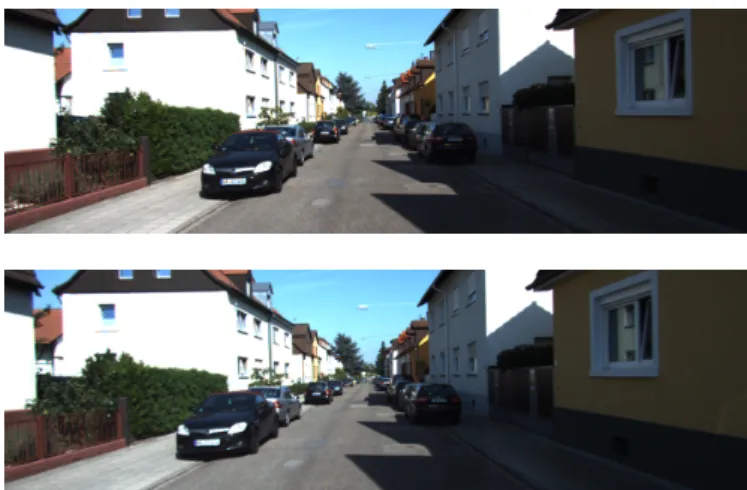
The first step is to capture an image pair from two cameras, and an example of such an image pair from the KITTI dataset [12] is shown in Figure 1.2. The basic principle of stereo vision is that two images are taken from different viewpoints. The relative horizontal position of a point in the two images, called the pixel disparity, can then be used to estimate the point’s distance from the sensor.
Figure 1.2: Example of a stereo image pair that can be used to estimate the distances of visible objects.
The process of finding such points in the two images is called the stereo correspondence problem, and is the focus of much research. The purpose of these techniques is to find the image correspondences as quickly as possible, without sacrificing the accuracy of the results. Measured disparities will inevitably contain errors, though, due to how difficult is it to find all corresponding points exactly.
The output of the stereo correspondence algorithm is a disparity map similar to the one shown in Figure 1.3, where a darker colour indicates a closer point and white points are not calculated. This disparity map collects all the measured disparity values calculated for an image pair. Using the disparity of a pixel, a point can be triangulated to real world coordinates. This process results in a cloud of 3D points that are measurements of objects in the environment.
Figure 1.3: Example of a disparity map.
If these measurements were perfect, these points could be used directly, but they are known to be imperfect. Therefore, a characterisation of the sensor – called an inverse sensor model (ISM) – is used that relates this noisy measurement to probabilities that an object is located at different positions.
An example of such an ISM is shown in Figure 1.4, displaying the likelihood that an object is located at different distances for a measured distance of 1 metre. It shows that since no objects were present in the range between the sensor and the measurement, this range is probably empty. Near the measurement the chances that an object exists are considerably higher, and for ranges further away from the sensor a value of 0.5 indicates that no information about the presence of objects is available. Using these probabilities, the inverse sensor model provides the information we use to update the map.
The occupancy grid mapping technique is a popular way to represent an environment [17–19]. It divides the environment into cells and assigns a probability to each cell that an object exists within it. These probabilities are updated over different measurements by using the probabilities calculated with the ISM. Visualising the probabilities of the map cells yields Figure 1.5, which shows the occupancy grid
0.0 0.5 1.0 1.5 2.0 distance from the sensor (m)
0.0 0.5 1.0 probabilit y of o ccupancy
Figure 1.4: Example of an inverse sensor model.
for a different example. In this visualisation, white indicates that a cell is empty, black indicates a cell is occupied by an object, and grey means that uncertainty exists about the occupancy of that cell.
Figure 1.5: Example of an occupancy grid map.
1.4
Thesis Overview
Firstly, we investigate the most prominent existing techniques and projects from the literature in Chapter 2. We make some design choices regarding which techniques to use for this study, and conclude with a detailed problem statement that specifies what this study hopes to accomplish.
In Chapter 3 we discuss dense stereo as a sensor for mapping, and analyse the measurement errors that some correspondence algorithms make using two different datasets. We expect that an accurate probabilistic characterisation of these errors should improve mapping.
We discuss mapping using an occupancy grid map discussed in Chapter 4, with specific focus on how new measurements are incorporated into the map. We also specify and explain the assumptions that we make.
After this, we investigate the modelling of the stereo vision measurements in detail in Chapter 5. When calculating the map, we need to accurately reflect the measurements errors, or else the result will not be reliable.
Results of testing the mapping system are shown in Chapter 6, where we analyse the maps. Lastly, we draw some conclusions about the study and suggest possibilities for further work in Chapter 7.
Chapter 2
Literature Study
Mapping on autonomous robotics with cameras has attracted great interest recently, partly due to advancements in computing power and optics. These developments have led to more advanced systems capable of previously impossible complexity. Some prominent and popular techniques from the literature are discussed in this chapter to offer an overview of the relevant fields. Section 2.1 gives a summary of some of the most prominent algorithms in stereo vision, Section 2.2 discusses various mapping techniques, and Section 2.3 highlights sensor modelling. After this, we investigate some related projects in Section 2.4, and provide a detailed problem statement in Section 2.5.
2.1
Stereo Vision
A method of measuring the distances that objects are from the sensor is an essential part of any au-tonomous mapping system. Stereo vision is a popular choice, since it offers large amounts of information per time step when compared to other methods such as sonar or radar, and is generally less expensive than LIDAR.
After discussing some core concepts required for stereo vision, we look at some common algorithms from the literature.
2.1.1
Core Concepts
The basic idea behind stereo vision is to use two cameras to estimate how far objects are. This is done by using the parallax effect, where objects viewed simultaneously from two parallel viewpoints appear in different positions [20]. Closer objects have a wider discrepancy in apparent horizontal positions.
Example images from two such cameras are shown in Figure 2.1. Any technique that uses an object’s disparity in two views can be labelled as stereo vision, but dense stereo is specifically when it attempts to calculate a disparity value for each pixel. The objective of a dense stereo algorithm is to construct a disparity map, which is a grid of disparity values with the same shape as the source image. An example of such a disparity map is shown in Figure 2.1(c).
One of the stereo images is usually considered as the reference image and the other as the target image. Finding disparity values is commonly referred to as the correspondence problem, since the aim is to find the corresponding positions in the target image for pixels in the reference image.
(a) (b) (c) Figure 2.1: Sample stereo images from the Tsukuba dataset [21].
The left and right stereo images are shown in (a) and (b), with the disparity map in (c) indicating the distance to each element
as a luminance value where lighter indicates further objects.
2.1.2
Common Algorithms
Calculating disparity values is not a trivial task and many different algorithms have been developed. It is complicated by a number of practical issues such as homogeneous areas in the environment, camera noise and bad lighting. It can also be difficult to find a universal method for quantifying and comparing similarities between image regions. For this study, some representative techniques that are suitable for autonomous mapping will be chosen from the literature.
A distinction can be made between localised and global methods [22, 23]. Localised methods find matching pixels by considering small areas around them in each image. Global methods consider the entire image and try to find matches for all the pixels simultaneously, usually by using energy minimisa-tion. This involves setting up a function that penalises certain unwanted aspects of matches, and then finding an optimal solution for it.
Another distinction is between sparse and complete techniques, where an algorithm that finds dis-parities more sparsely results in less data. These results tend to be more accurate, though, since any pixel for which a clear match cannot be found is marked as incalculable.
Algorithms also make a trade-off between accuracy and execution speed. For our application the stereo matching will need to be fast to allow for online calculation, but if the values are not sufficiently accurate it may not be suitable to mapping.
2.1.2.1 Block Matching
The block matching algorithm of Konolige [24] is based on the classic correlation-based technique that has been used extensively [25, 26]. It is a local method that considers areas around the considered pixels in the two images to find the best matches.
Pixel comparisons are done by calculating the correlation between surrounding areas. The point of maximum correlation then relates to the part of the target image that most resembles the area around the reference pixel. Subpixel accuracy can be achieved in block matching by fitting a quadratic curve to a few best matches and solving for the local maximum.
The size of the area considered has a significant impact on the result, since a smaller area will be more likely to match and a larger area will result in a smoother result. Therefore the block matching technique requires some tweaking for a given application to perform optimally.
2.1.2.2 Semiglobal Block Matching
Semiglobal block matching, as developed by Hirschm¨uller [27], extends upon the block matching tech-nique by also considering the disparity values of surrounding pixels. This leads to smoother, less noisy disparity maps, assuming that the distances to visible objects vary mostly smoothly.
The extension is done by minimising an energy function that considers not only the area around pixels as before, but also the local changes in disparity that a possible match would cause [28]. The function is calculated as the sum of the energy costs for a number of paths from different directions to the pixel in question, and for a defined range of possible disparity values. This leads to a range of energy costs at each pixel – one per possible disparity value – and the minimum cost found represents the best match.
Semiglobal block matching requires a more complex calculation process than traditional block match-ing, which leads to a longer execution time. Since it is not fully global, however, it still offers direct solving as opposed to an iterative solution that would require a series of approximating results.
2.1.2.3 Dynamic Programming
The first application of dynamic programming to stereo vision was done by Ohta and Kanade [29], matching stereo images by comparing pixels directly and considering the edges between different visible objects. This process involves repeatedly subdividing the image into smaller pieces and matching each piece separately before combining the results, which significantly reduces the complexity of the solution. The problem with this simplification is that it assumes independence between the lines in the image. Each line in the reference image is matched individually, which means that the calculated disparity map is not necessarily smooth.
2.1.2.4 Belief Propagation
A more modern development in stereo vision is to make use of Markov random fields to model the similarities between the left and right images. Each random variable in the field represents the disparity of a particular pixel. Edges are defined between adjacent pixels and describe the relationships between them, to define local smoothness. One of the techniques for finding the lowest global matching cost in such a Markov random fields is belief propagation, as first described by Sun et al. [30].
The problem with belief propagation is that it requires iteration to converge to a solution, which makes it inconvenient for online calculation. Yang et al. developed it further by using a constant space algorithm [31], where the same memory is reused to limit the amount of data being stored. This led to significant reductions in the execution time and memory usage, but also decreased the accuracy of results due to further approximations.
2.1.2.5 Variational Matching
Variational matching also balances smoothness with locally accurate matching, combining costs for the differences between local areas around pixels with a smoothness constraint [32]. It compares regions around pixels by calculating the sum of squared differences. Smoothness is ensured by employing a regulariser that uses the gradient of the disparity map to ensure minimal local disparity variations. This smoothness value is then added to the data cost to create the energy function, which is solved by defining the disparity map as an Euler-Lagrange equation [33] and solving the resulting partial differential equation.
It is a local method, offering very fast calculation times and low memory usage. Results are fairly accurate [32] with some fuzziness at depth borders.
2.1.2.6 Conclusion
For the purposes of this study a few techniques are chosen for further investigation, representing both local and global, dense and sparse, as well as accurate and inaccurate techniques. We choose block matching, semiglobal block matching and variational matching. Although other techniques such as belief propagation offer very accurate results, they rely on iteratively solving large scale optimisation problems and do not offer practically feasible solutions for online mapping. Furthermore, implementations for the chosen techniques are available in the open source OpenCV library [34].
2.2
Mapping
An autonomous vehicle that navigates and investigates its surroundings autonomously needs a way to represent its environment given measurements. This is commonly done using a map that is capable of describing a region. Preferably, this should be in a memory efficient way which would allow for larger areas to be explored in more detail.
Some commonly used mapping techniques are discussed here to find the best option based on the requirements of this application. Each mapping technique will be evaluated based on its ability to store large amounts of data efficiently and accurately, the accessibility of its information, and how flexible the stored map is. To be considered flexible, it must be extendible when additional areas are explored, and its resolution should be variable so it can fit many different applications.
2.2.1
Point Clouds
The naive way to represent data points in world coordinates is to use a point cloud, where every known point in the map is represented with a 3D coordinate. Although it offers a very simple way to represent information and does not require additional processing, it provides limited usability for navigation and processing techniques due to the complexity of accessing information about a particular region [35].
The problem with point clouds is that they do not combine measurements that represent essentially the same information, and therefore its memory usage can grow without bound. Eventually, many points will contain redundant information.
Pan et al. [36] showed that it is computationally expensive to do collision detection with point clouds, since each point has to be considered individually. In order to know if an obstacle exists at a specific point, or to find the closest data point to a coordinate, every existing data point needs to be queried (leading to a complexity of O(n2)). Some simple improvements, such as combining points
that lie close together or labelling data based on location using KD-trees, can be made to simplify usage. However, sophisticated processes like path planning are unnecessarily complicated when the environment is represented with individual points.
2.2.2
Topological Maps
One way to reduce the amount of data stored is to create a topological map [37, 38] that represents the environment with a graph. It works similarly to a roadmap, creating nodes of known or important points and connecting them with edges that represent pathways. This simplification makes topological maps
difficult to use, and some data is lost. For instance, they do not indicate the locations of objects and hence cannot be used for collision avoidance.
The graph that describes the map is very efficient to traverse, since each node is only connected to a few others. This makes them convenient to use for navigation algorithms, where paths through the graph are often used to represent possible routes. Applications of this also includes transport networks like rail systems or subways.
Another issue with topological mapping is its inability to represent uncertainty. Although it represents known positions well, it is hard to distinguish between empty space and unknown areas.
2.2.3
Occupancy Grids
Currently the most popular solution for mapping used in robotics is the occupancy grid mapping tech-nique that represents an environment as a tessellated map1 consisting of a number of 2D squares or 3D cubes [19, 39, 40]. The technique was originally coined by Elfes, who created a probabilistic imple-mentation capable of creating 2D or 3D maps [39]. He also developed a method of incorporating the uncertainty in measurements from sonar and stereo vision sensors by modelling their errors.
The basic principle of an occupancy grid is to discretise the world into a number of cells and assigning each a binary classification [41] where it can be either occupied or empty. To incorporate uncertainty into the representation, the classification is stored as a probability, where 1 indicates that it is definitely occupied, 0 indicates it is definitely empty and 0.5 that no information about its occupancy is available. The technique is developed specifically to map static environments that do not change, since mapping dynamic objects entails an entirely different approach where dynamic object are identified and tracked over time.
The original implementation divided the environment into equally sized blocks and stored only a probability that each contained an obstacle. This could result in a large number of superfluous homo-geneous neighbouring blocks, which was improved by adaptive grid mapping. This is implemented by transforming the map into a tree-based structure, as described by Einhorn et al. [42] and shown in Figure 2.2.
Root node
Leaf nodes
Leaf nodes
Figure 2.2: Example of a tree-based occupancy grid, showing a root node that is divided into smaller nodes.
The top level node is referred to as a root node, is the largest map cell in the tree and has the same size as the entire tree. Any node not divided into children is called a leaf node as marked in Figure 2.2, and in most implementations a probability of occupancy is calculated for these leaf nodes. Homogeneous regions can be merged by pruning sections of the tree that do not provide additional information. This improves the memory usage of the map, especially when mapping in 3D. Additionally, when some measurements
1This tessellation means that the map consists of a number of cells (not necessarily all the same size) that fit together without gaps or overlapping.
indicate a cell is occupied and others that it is empty, that cell may be divided into smaller cells. Each of these cells can be assigned its own probability of occupancy, which allows the map to represent complex regions in greater detail.
Occupancy grids are the obvious choice for mapping in this study, due largely to its popularity in the field of autonomous mobile robotics. Most recent projects (see Section 2.4) have used it due to its efficient memory usage and elegant implementation.
It represents the environment in a convenient way, since many navigation and collision avoidance algorithms were developed to work on such a grid-based representation. Since any point in the map can be queried directly based on the probability that it contains an object, these algorithms can easily use the map to establish the safety of specific paths.
Importantly, it offers a way to model the uncertainty in the state of a map cell, which is crucial with inaccurate sensors such as stereo vision. Mapping using occupancy grids is reliant on the inverse sensor model that is discussed in Section 2.3.
2.3
Sensor Models
The sensor model is an important part of the occupancy grid mapping technique. It describes a relation-ship between a map and measurements made of the environment. Sensor models are also responsible for representing measurement noise, since they affect the way that measurements relate to the environment. We update the occupancy probability of each map cell using the sensor model to find a distribution based on the new measurements, and then incorporating that distribution into the existing belief.
The forward and inverse sensor models are discussed next.
2.3.1
Forward Sensor Model
The forward sensor model is described and used by Thrun [40]. It specifies a probability distribution over sensor measurementsz given a mapm. It is of the form
p(zt|m), (2.1)
wherezt refers to the measurements at a certain time step andmto a map. The forward sensor model in essence describes the measurement for every possible combination of the map.
The way Thrun calculates maps using the forward sensor model involves an iterative solution. Essen-tially, maps that are likely to have caused a set of measurements are searched for using the expectation maximisation (EM) technique [43]. A number of other forward models exist, however, specified in dif-ferent ways.
In Section 3.5 of his paper, ?? describes how he estimates the marginal posteriorP(mxy, Z). Another problem with this algorithm is that maps are found based on the full set of measurements, making it computationally intractable to update the map every time new measurements become available. Ideally a robot should be able to calculate a map incrementally as it explores, allowing the map to be used as it is created.
An alternative way to learning occupancy grid maps with forward sensor models was proposed by Pathak et al. [44]. The authors use forward sensor models for incremental mapping, without iteratively solving maps. This approach does not explicitly calculate occupancy probabilities, and instead establishes probabilities of visibility. This has been found to be an inferior solution when compared to algorithms
that establish occupancy probabilities [45].
2.3.2
Inverse Sensor Model
The inverse sensor model, in turn, is given by
p(mi|zt), (2.2)
and models the distribution of a map cell mi given one time step’s measurements zt. This is not the causal direction since the map cells’ states of occupancy are not caused by the measurements, which is what gives the inverse sensor model its name.
The inverse sensor model was created as part of the occupancy grid mapping technique by Elfes [46], and extended by Thrun [17]. A number of alternative models have also been suggested [47, 48]. All these models have been used to create occupancy grid maps incrementally, usually using close range sensors such as sonar or lasers.
However, a principled derivation is not available for the inverse sensor model, as the available models seem to be chosen empirically. In general, the existing models are also limited by an assumption of unimodal Gaussian noise.
Due to the reasons discussed here, we focus on the inverse sensor model rather than the forward sensor model. We discuss it in detail in Chapter 5, where we also provide a derivation.
2.4
Related Projects
Using stereo vision as an input to mapping has recently received considerable academic attention, since advancements in processing power improved the image processing possible on mobile robots. A number of prominent examples from the literature are discussed here.
Some projects focus on mapping, for instance the Octomap occupancy grid mapping implementation [49] that offers a common framework for 3D mapping. Although it offers an efficient and convenient way to create maps, it is limited by an ideal sensor model that does not incorporate the uncertainty in measurements. Alternatives to the Octomap framework include the work done by Schauwecker and Zell [50], who employ a linear sensor model. Although an improvement upon the modelling in Octomap, this is inadequate for the measurement uncertainty in most practical sensors.
Most of the projects that implement mapping on board a mobile robot limit it to 2D occupancy grid maps [15, 51, 52]. Although sufficient for simple robot models that only consider planar movement, this can be problematic in more complex environments or with vehicles capable of moving in more than two dimensions.
The u-disparity plane [51] can be used to simplify the integration of stereo data into the global map. This is done by effectively reducing the dimensionality of the disparity map before integrating it into a 2D map. Although very efficient and useful for navigation, since large areas around obstacles are considered occupied, this technique is only viable for simple environments.
An alternative to 2D mapping is creating a 2.5D (also known as occupancy-elevation) grid map as done by Souza and Maia [53]. Instead of assigning an occupancy to each cell in a 2D grid, a Gaussian distribution is created that describes the heights of obstacles in that cell. Although this is much simpler and faster to calculate than a full 3D occupancy grid map, it contains significantly more information about obstacles than the standard 2D representation, which can be useful for navigation.
Apart from some projects that employ simple sensor models [54, 55], one of the first studies to successfully use stereo vision as input for a 3D map was done by Andert [47]. A novel sensor model is used to create 3D maps in adequate detail to autonomously navigate a remote controlled helicopter that is used in testing. However, this sensor model is provided without a principled derivation, and is limited to zero-mean Gaussian sensor noise.
Some modified versions of Andert’s sensor model exist, such as the work done by Heng et al. [56], where the model is forced symmetrical around the measurement with a quadratic exponential. This is done to assign an equal occupancy probability to grids at equal distances around the measurement, without clear justification. As shown by Matthies and Shafer [57], however, the sensor model should be asymmetrical around the measurement location due to the exponential nature of stereo sensor error over distance.
2.5
Detailed Problem Statement
The problem that we focus on is creating reliable 3D maps using stereo vision as a sensor. A survey of the literature indicated that such a system is not available, with most of the existing implementations focusing on real-time calculation. There is often a direct trade-off between execution speed and accuracy. Many implementations make strict assumptions about the accuracy and range of the sensor, which puts strong limitations on the mapping system.
Using stereo vision as a sensor for mapping entails processing the images with a stereo correspondence algorithm, the results of which are known to be noisy. Triangulating these points to real world coordinates can cause more distant measurements to be very inaccurate, which can be problematic if the uncertainty in these measurements is not considered carefully.
Therefore, we wish to create a way to characterise the measurement errors made by a stereo cor-respondence algorithm. This characterisation should describe the error distribution, which must be incorporated into the sensor model so measurements can be reliably integrated into the map.
Since existing sensor models are generally limited to zero-mean Gaussian noise, we wish to derive an inverse sensor model that is capable of describing more complex sensor noise distributions. Considering the complexity of the stereo correspondence problem, we need a sensor model that is capable of capturing the uncertainty in such measurements. If such a sensor model is not available, it can lead to overconfidence in the calculated map.
We will follow a principled approach to deriving the inverse sensor model, ensuring that the assump-tions we make are clear and physically meaningful. This should result in an inverse sensor model that is not chosen empirically, but instead comes from sound statistical principles.
Chapter 3
Stereo Vision
Retrieving distances to visible objects from a stereo camera sensor requires a solution to the correspon-dence problem. Due to the cameras and the rig itself being non-ideal some calibration and correction need to be done before this is possible. Even then, a correspondence algorithm may return erroneous disparities that must be characterised so they can be used reliably in the construction of a map.
Before the disparity errors are considered, a brief explanation of the geometry involved in stereo vision is provided in Section 3.1. After this, some of the issues faces by correspondence algorithms are discussed in Section 3.2. Lastly, the error characteristics of these algorithms are investigated in Section 3.3.
3.1
Stereo Vision Geometry
Most techniques used to solve the correspondence problem in stereo vision rely on a simplified model of the geometry. Before these techniques can be implemented the images need to be transformed to fit this model.
This process is detailed here by first explaining the concept of homogeneous coordinates, and then detailing the pinhole camera model. The relevant mathematics for projecting points onto the images is included, accompanied by a short description of how a camera can be calibrated. After this, we briefly describe how points can be triangulated to world coordinates, and how we rectify stereo images to simplify triangulation.
Most of the theory in this section is based on work by Bradski and Kaehler [34] and Hartley and Zisserman [58].
3.1.1
Homogeneous Coordinates
In homogeneous notation, [x1 x2 x3]T represents not only a single vector, but a collection of scaled
vectors k[x1 x2 x3]T where k 6= 0. When all these classes are combined it forms the projective space P2, and allows for the representation of infinities in the far field. This spaceP2is the set of lines inR3
passing through the origin.
Any 2-dimensional vector [x1 x2]T can be written in homogeneous coordinates as [x1 x2 1]T by
projecting them onto thez = 1 plane, and a homogeneous vector [x1 x2 x3]T can be written inR2 as
[x1
x3
x2
x3]
T as long asx
36= 0. This also extends to a 3-dimensional vector inR3 that can be written as a
3.1.2
Pinhole Camera Model
The pinhole camera model is fairly simple, and is used in almost every computer vision system that requires a mathematical model for camera projection. It describes how points are projected onto an image, and is integral to the geometry of stereo vision. A brief summary is given here, and the reader is referred to the work by Hartley and Zisserman [58] for more information.
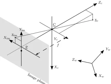
The main objective of the pinhole camera model is to project a point in 3D onto an image plane. This projection is shown in Figure 3.1, which details the projection of a point in camera coordinates xc = [xc yc zc]T through the camera centre C onto an image plane with origin at the principal point p. It also shows the world coordinate system, which differs from the camera coordinate system by some rotation and translation. This geometry is also commonly drawn with the image plane between the camera centre and the point being projected.
xc Xc Zc Xim xim Yim Image plane f Yc C Zw Yw Xw p
Figure 3.1: Illustration of the pinhole camera model, showing a point in camera coordinates projected onto the image plane.
The projection from the point in world coordinates (xw = RTxc+ C for some fixed rotation matrix R that relates the camera coordinate frame to the world coordinate frame) onto the image plane is described in homogeneous coordinates with the equality
xim= Pxw. (3.1)
Here P is the projection or camera matrix, of the form
P = KR[I |−C]e , (3.2)
where C is the Euclidean form of the camera centre in world coordinates. The matrix K is called thee
calibration matrix and contains the intrinsic parameters of the camera. It is of the form
K = αx s x0 0 αy y0 0 0 1 , (3.3)
withαxandαyscaled versions of the focal length that also account for scaling between world coordinates and pixels, x0 and y0 the pixel coordinates of the principal point (where the camera’sZ-axis intersects
the image plane), andsa skewness factor.
Equation 3.1 provides a way of projecting a point in world coordinates onto the image plane, given the intrinsic parameters described in K and the extrinsic parameters described by R andC.e
3.1.3
Calibration
When we use the pinhole camera model for stereo vision, we rely on two camera matrices P and P0, where P is the projection matrix for the left camera and P0 the right camera’s projection matrix. Together these matrices encapsulate the intrinsic and extrinsic parameters of the two cameras. These values are not only dependent on the cameras, but also on how they are set up relative to each other and to the vehicle.
Calibration of the stereo vision sensor amounts to finding P and P0. This process and its automation have been detailed in the literature [34]. It usually involves capturing images of an object with known dimensions (often a planar checkerboard).
3.1.4
Triangulation
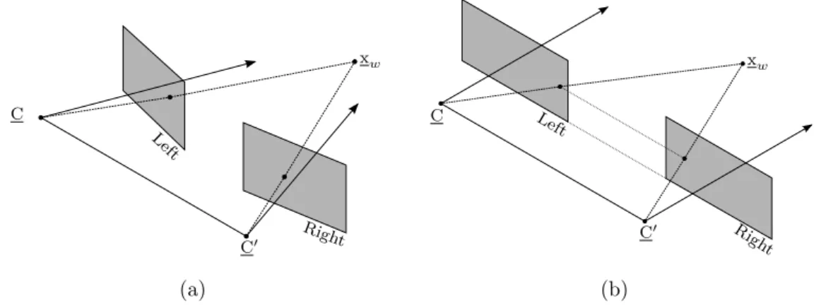
The main purpose of stereo vision is to triangulate a point to 3D world coordinates from its projection on two image planes. This can be performed by solving for xwfrom the homogeneous equations xim= Pxw and x0im = P0xw, given xim and x0im [59]. Instead of following that route, it is better to first transform the two images through a process called rectification. This simplifies not only triangulation but also the correspondence problem , since corresponding points in the two images will be in the same row.
3.1.5
Rectification
Triangulation and indeed the correspondence problem can be simplified by a process called rectification, which ensures that matching points in the two images are in the same image row. An example of this is shown in Figure 3.2, where two stereo image planes are rectified to align the image rows.
C C0 xw Left Righ t C C0 xw Left Righ t (a) (b)
Figure 3.2: Rectification of stereo image planes, showing (a) the original image planes and (b) the rectified ones.
Provided both camera matrices P = KRhI | −Ce i and P0= K0R0hI| −Ce 0i (3.4)
are available, we define new projection matrices Pn= KnRn h I| −Ce i and P0n= KnRn h I| −Ce 0i . (3.5)
Here the two cameras not only have the same intrinsic camera parameters (Kn), but their orientations relative to the world coordinate system (Rn) are also the same. The only thing that differentiates the two camera matrices is that they have different camera centres in world coordinates (C ande Ce
0
). We choose Kn as the average 0.5(K + K0), and determine the rotation matrix Rn aligned with the vector between the two camera centres (Ce
0 −C).e
The two captured images are transformed with the homographies T1= KnRnRTK−1 and T2= KnRnR0
T
K0−1. (3.6)
When these transformation matrices are applied to the respective images, it results in two rectified images with aligned image rows.
This means that any point in space that is triangulated to two rectified image planes yields a com-munal yim coordinate, and two distinct xim coordinates. The difference between these xim values (the
disparity) can be used to triangulate the rectified image coordinates back into world coordinates.
3.1.6
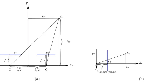
Simplified Triangulation
The required values for triangulating a point [xn yn zn]T into the rectified camera coordinates are the projected locations [xL y]T and [xR y]T, the baseline (distance between the two camera centres)b and
the rectified focal lengthf of the cameras. From similar triangles in Figure 3.3 it is known that
f xL = b zn 2+xn and f xR = zn xn−2b , (3.7)
where the coordinatesxL andxR are the projected horizontal pixel locations. Introducing the principal
point, which is the pixel offset of the optical axis on the image plane yields
xn= (xL−px)b xL−xR −b 2, yn= (y−py)b xL−xR and zn= f b xL−xR . (3.8)
3.2
Common Sources of Errors in Dense Stereo
The stereo correspondence problem is difficult to solve, and any algorithm will inevitably make mistakes. We define these errors by subtracting the calculated disparity value (xL−xR) from the ground truth,
both in pixels. This leads to a measurement error measured in pixels, where a positive value indicates that the ground truth value is larger and therefore that the stereo correspondence algorithm estimated
Xn Zn xn C b/2 b/2 C0 xL xR xn zn f f xn f Image plane y zn yn Zn Yn (a) (b)
Figure 3.3: Simplified geometry used to triangulate matching points in rectified stereo images.
the object too far away.
The problem is that even disparity errors of a few pixels can be problematic, since the real world distance is inversely proportional to the pixel disparity according to Equation 3.8. Figure 3.4 shows that although a small pixel error will translate to a small error in distance at close range, the same pixel error will relate to a greater distance error if the obstacle is far away.
0 20 40 60 80 100
disparity (in pixels) 0 20 40 60 80 100 120 140 160 distance from sensor (in meters)
Figure 3.4: Typical inverse proportional relationship between pixel disparity and distance.
Although each stereo algorithm can have its own error characteristics, there are a number of problems that are common to all. Most of these problems occur due to the nature of the correspondence problem, while others are due to more practical aspects of solving it.
3.2.1
Bad Rectification
One possible cause of errors is inaccurate rectification. Local matching algorithms in particular rely on a strong alignment between the same rows in the two images.
This problem leads to either many points for which the correspondence problem cannot be solved in sparse techniques, or large errors if the algorithm is dense. Dense algorithms attempt to find the
correspondence of a pixel in a winner-takes-all manner, which can cause problems if a good match is not found.
3.2.2
Occlusions
Occlusions are an effect of the difference in viewing angles of the two cameras, and causes points to be visible to one camera and not the other. Stereo vision algorithms function on the premise of finding objects in the target image that are visible in the reference image, which is impossible if objects are occluded. Apart from the obvious case where one camera’s view of an object is obstructed, occlusions also occur at the boundaries between objects at different distances.
It is almost impossible to identify occlusions once the stereo correspondence algorithm is complete, since the errors they cause are not predictable. One technique that has been found to be effective is dual matching [60], which involves independently matching not only the target image to the reference image, but also the reference image to the target image. It amounts to twice as much processing, but occlusions should appear as differences between the two calculated disparity maps.
3.2.3
Uniformity
Possibly the greatest challenge for outdoor stereo vision systems is lack of texturing, where uniform regions such as the sky or the walls of buildings do not contain enough information for matching. A stereo vision algorithm relies on finding corresponding pixels or regions in two images, which is impossible if the images contain large areas that are homogeneous.
The result of matching these areas can contain large errors, which can be catastrophic for mapping. Some algorithms put smoothness constraints on calculated disparities (under the assumption that nearly all scenes comprise piecewise smooth surfaces), which may limit these types of errors.
3.3
Characterisation
Different stereo correspondence algorithms work in different ways. To facilitate the accurate mapping of an environment with erroneous measurements, we need a way to model the errors in the output of a particular stereo correspondence algorithm for a given setup and environment. If this characterisation is incorporated correctly into the inverse sensor model, then the calculated occupancy probabilities should capture the uncertainty in the measurement.
To find this model, we measure the errors made by a stereo algorithm over a representative subset of data, provided that ground truth is available. We then bin these errors into a histogram to calculate the relative frequencies of different errors. However, we need a probability density function to approximate this error histogram, which we can use to set up the inverse sensor model.
A Gaussian mixture model (GMM) is a model consisting of Gweighted Gaussian components that are summed, and is written as
p(x) = G X i=1 wi 1 p 2πσ2 i exp −(x−µi) 2 2σ2 i , (3.9)
where theith component is described by its relative weight wi, its mean µi, and its standard deviation
a given distribution. The component weights satisfy the constraints that G
X
i=1
wi= 1 and wi≥0. (3.10)
Given enough components, GMMs are known to be able to smoothly approximate distributions of any shape [43].
We choose to use a GMM to describe the error distribution in this study for its generality, and employ it here to approximate the error distributions of the three algorithms identified in Section 2.1.2 on two different datasets. The expectation maximisation (EM) technique [43] is used to fit GMMs with varying numbers of components to the error histogram of each algorithm on each dataset. The number of components G in the GMM is a trade-off between over-specialisation and reducing execution time with fewer components.
An important assumption we make is that the disparity error is independent of position in the image. This allows for the creation of a single model that provides a distribution for the error in every measurement from the sensor.
Each calculated GMM is shown with the histogram of the error of the respective stereo algorithm for qualitative evaluation, and details of each GMM are provided in a table. This includes the parameters for each of the calculated components, as well as the Akaike information criterion (AIC) [61] which provides a relative quality of fit to models for a given set of data. The AIC of a GMM fitted to data is defined as
AIC =−2log(maximum likelihood) + 2(G), (3.11)
and is designed to weigh a model’s quality of fit against its complexity. Here the parameterGis again the number of components in the fitted GMM, and the maximum likelihood is the likelihood that the given model resulted in the data provided. Although the value itself does not have a clear physical meaning, it can be used for model selection, since a model that fits data better will have a lower AIC value.
We apply the three stereo correspondence algorithms identified in Section 2.1.2 to the synthetic Tsukuba dataset [21] and characterise the errors. Since the system is being developed for outdoor mapping, the KITTI dataset [12] is used for testing as well, since it offers rectified stereo images of urban scenes.
3.3.1
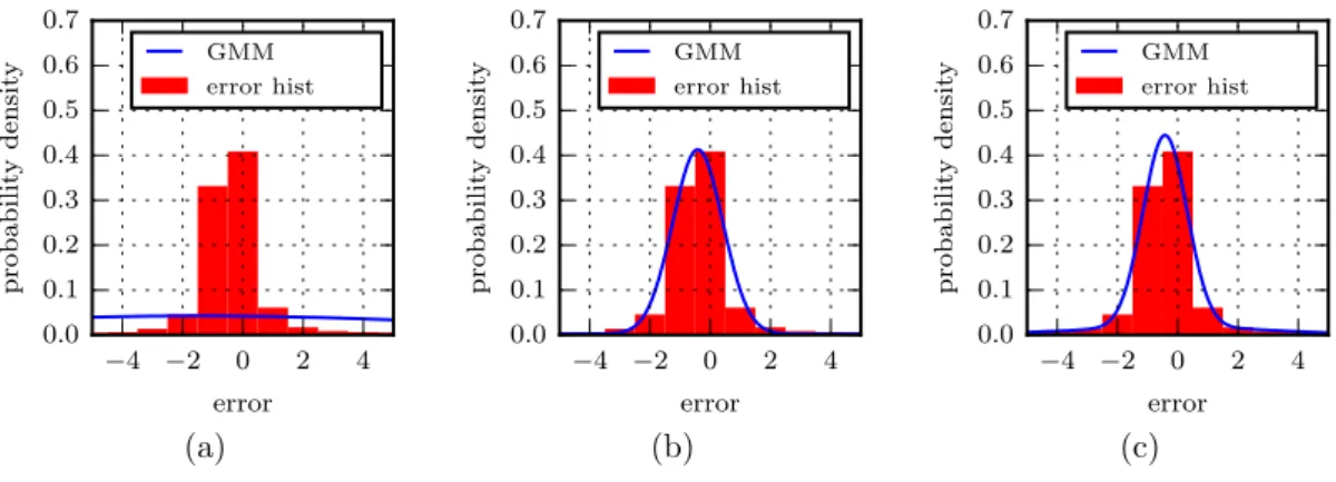
Wide Error Distributions
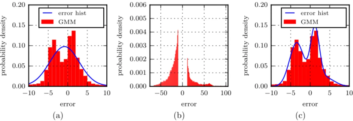
The EM algorithm we use to fit GMMs can be sensitive to outliers in wider error distributions. Increasing the number of components in the GMM should solve the problem with outliers, but it means that we can require many components in the GMM if the distribution contains multiple small components. In an effort to represent the original error distribution as well as possible, we fit GMMs using all available error values.
This issue is illustrated in Figure 3.5, where a GMM is fitted to a set of data. Although the first histogram suggests that the distribution consists of two components, even the GMM fitted with three components appears to be a bad fit. The part of the histogram that is outside the range shown in Figure 3.5(a) is shown in Figure 3.5(b), and indicates that although relatively small, other components exist in the distribution. Removing these values and fitting a GMM with three components to the remaining data results in the model shown in Figure 3.5(c), which appears to be a significantly better fit.
−10 −5 0 5 10 error 0.00 0.05 0.10 0.15 0.20 probabilit y densit y error hist GMM −50 0 50 100 error 0.000 0.001 0.002 0.003 0.004 0.005 0.006 probabilit y densit y −10 −5 0 5 10 error 0.00 0.05 0.10 0.15 0.20 probabilit y densit y error hist GMM (a) (b) (c)
Figure 3.5: The effects of wide distributions on fitting a GMM with EM, (a) shows the original 3-component GMM, (b) the
wider values and (c) a model fit only to the data shown.
many more components when fitting a GMM with EM. For example, a 7-component GMM is required to visually represent the data presented in Figure 3.5. The similarity between the AIC values of the 7-component model and the 3-component model suggests that they offer similar fits.
When we provide the parameters of GMMs in tables in this thesis, we describe the models fitted with one, two, and three components, as well as the first model that visually resembles the data (in the example case this would be the 7-component model). The last model is represented using only its components that have weights of more than 0.1.
3.3.2
Synthetic Data
The synthetic stereo dataset from Tsukuba University [21] is chosen for testing, since it contains cali-brated and rectified stereo images as well as ground truth for the dense disparity maps. The first 100 pairs of stereo images from the collection of 1800 are used for characterisation, their measurement error values are collected for a specific stereo algorithm, and a number of GMMs are fitted. The number of error data points collected from these images vary from 6.9 million for block matching to 20 million for denser algorithms such as the semiglobal block matching algorithm.
The scene in this dataset is the inside of a simulated office building, starting at the familiar bust from the Middlebury set [62] shown in Figure 3.6(a). Since the dataset is computer generated it contains many areas that are not textured, which could cause problems for the correspondence algorithms.
The ground truth is available and an example frame is shown in Figure 3.6(b), with darker areas indicating objects nearer to the sensor. The ground truth contains disparity values that cannot be calculated by any stereo algorithm (areas with occlusions or no textures). This should favour sparser algorithms, provided they are capable of correctly identifying such areas as incalculable. The result of the three stereo correspondence algorithms is shown in Figure 3.7.
3.3.2.1 Block Matching
The first technique for which the characterisation is tested is block matching, which calculates fairly sparse disparity maps. The histogram of its errors is shown in Figure 3.8, with GMMs fitted with varying numbers of components. The block matching algorithm appears to calculate accurate disparity values, but the single component GMM is badly affected by the problem in Section 3.3.1. The parameters for the models are shown in Table 3.1, and indicate that each of the fitted models consists largely of a
(a) (b)
Figure 3.6: Sample image from the Tsukuba dataset [21] with (a) from the left camera and (b) the corresponding ground truth
disparity map.
(a) (b) (c)
Figure 3.7: Disparity maps with differently scaled intensities for the Tsukuba dataset. (a) shows block matching, (b) semiglobal
block matching, and (c) variational matching.
single component, and that other components are negligibly small.
The models fitted to the errors produced by the block matching algorithm are dominated by a single Gaussian component with standard deviation around 1 pixel. It suggests that for this algorithm the existing sensor modelling techniques mentioned in the literature study would be adequate, although a small mean offset is present that they would be incapable of representing. Due to the increased tightness of fit that the third component introduces, the 3-component GMM should be the best option.
3.3.2.2 Semiglobal Block Matching
The second technique is the more global and more complete semiglobal block matching.
Resulting characterisation is shown in Figure 3.9. The errors seem to be largely around zero, with
G AIC µ1 σ1 w1 µ2 σ2 w2 µ3 σ3 w3
1 5.33×10⁷ −0.80 4.04 1.00
2 3.00×10⁷ −0.38 1.07 0.92 −5.67 20.68 0.09
3 2.75×10⁷ −0.35 0.64 0.86 −1.48 4.49 0.11 −10.28 31.16 0.03
Table 3.1: Parameters of block matching GMM for the Tsukuba dataset, withGthe number of components
−4 −2 0 2 4 error 0.0 0.1 0.2 0.3 0.4 0.5 0.6 0.7 probabilit y densit y GMM error hist −4 −2 0 2 4 error 0.0 0.1 0.2 0.3 0.4 0.5 0.6 0.7 probabilit y densit y GMM error hist −4 −2 0 2 4 error 0.0 0.1 0.2 0.3 0.4 0.5 0.6 0.7 probabilit y densit y GMM error hist (a) (b) (c)
Figure 3.8: Error distribution from the block matching algorithm on the Tsukuba set. (a), (b) and (c) show GMMs with one to three components respectively. Note that only the
section with non-negligible sized components is shown.
a standard deviation of roughly 1 pixel. A 2-component GMM seems to fit the data fairly accurately. This is further shown in Table 3.2, where the parameters for each of the calculated GMMs are detailed. There is a dominant component with zero mean and a standard deviation of roughly 0.7 pixels.
−4 −2 0 2 4 error 0.0 0.1 0.2 0.3 0.4 0.5 0.6 0.7 probabilit y densit y GMM error hist −4 −2 0 2 4 error 0.0 0.1 0.2 0.3 0.4 0.5 0.6 0.7 probabilit y densit y GMM error hist −4 −2 0 2 4 error 0.0 0.1 0.2 0.3 0.4 0.5 0.6 0.7 probabilit y densit y GMM error hist (a) (b) (c)
Figure 3.9: Error distribution from the semiglobal block matching algorithm for the Tsukuba set. (a), (b) and (c) show
GMMs with one to three components respectively. Note that only the section with non-negligible sized components is shown.
The error distribution of the semiglobal block matching algorithm could also be represented by a single component, although it benefits from a second component due to the presence of a small but very wide component in the distribution. Although the 2-component and 3-component GMMs offer similar fits, the GMM withG= 3 seems to be the best option.
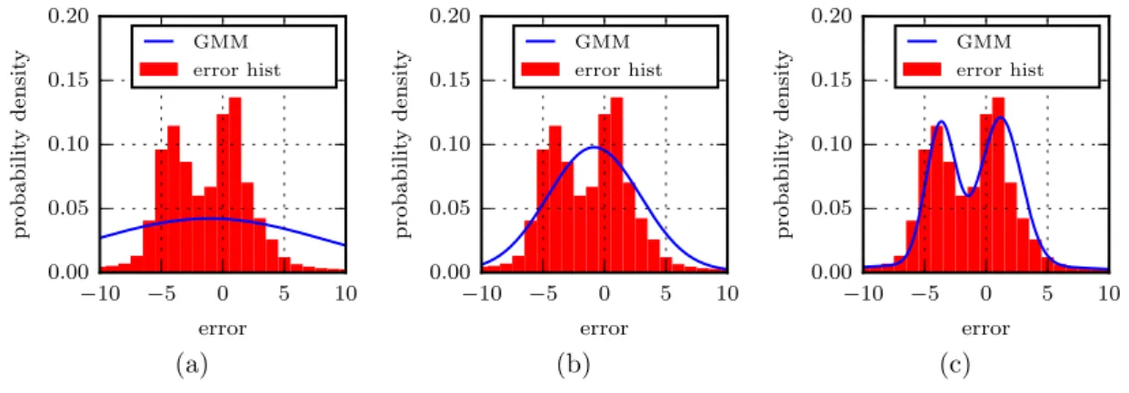
3.3.2.3 Variational Matching
The variational algorithm offers dense disparity maps that can be calculated very quickly but with the compromise of large errors being made. The resulting disparity maps are smooth due to the area-based design of the technique.
The characterisation is illustrated in Figure 3.10, showing the different GMMs fit to the error his-togram. The error distribution seems more complex than that of the other algorithms, with the intro-duction of more components to the GMM resulting in significantly different models. The GMM with
G AIC µ1 σ1 w1 µ2 σ2 w2 µ3 σ3 w3
1 1.83×10⁸ −1.48 9.34 1.00
2 1.71×10⁸ −0.42 0.78 0.86 −7.74 23.50 0.14
3 1.71×10⁸ −0.42 0.67 0.78 −0.15 3.00 0.13 −12.08 28.15 0.09
Table 3.2: Parameters of semiglobal block matching GMM for the Tsukuba dataset.
nine components is included because it is the first one to distinguish between the two secondary peaks of the distribution. 0 5 10 15 20 25 30 error 0.00 0.05 0.10 0.15 0.20 probabilit y densit y GMM error hist 0 5 10 15 20 25 30 error 0.00 0.05 0.10 0.15 0.20 probabilit y densit y GMM error hist 0 5 10 15 20 25 30 error 0.00 0.05 0.10 0.15 0.20 probabilit y densit y GMM error hist (a) (b) (c)
Figure 3.10: Error distribution from the variational matching algorithm on the Tsukuba set, characterised with different GMMs. (a) (b) and (c) show GMMs fitted with two, three and
nine components respectively. Note that only the section with non-negligible sized components is shown.
The calculated parameters are shown in Table 3.3, where the first four parameters for the 9-component GMM are displayed. These are the largest components of the GMM and represent 63% of the total weight, where the other components each have weights smaller than 0.1. According to how the AIC measures quality of fit, the GMMs with three and nine components are suggested to have similar qualities of fit. However, we prefer the 9-component model since it appears to be more similar.
G AIC µ1 σ1 w1 µ2 σ2 w2 µ3 σ3 w3 µ4 σ4 w4
1 2.50×10⁸ 7.35 13.75 1.00
2 2.35×10⁸ 8.86 6.04 0.76 2.80 25.22 0.24
3 2.26×10⁸ 5.38 1.38 0.38 14.33 4.59 0.32 2.55 22.78 0.30
9 2.24×10⁸ 5.75 0.80 0.24 17.88 2.57 0.14 11.59 3.67 0.13 9.09 12.33 0.12
Table 3.3: Parameters of variational matching GMM for the Tsukuba dataset
The Gaussian mixture model seems to be capable of representing the error distributions for all three stereo algorithms. Although a GMM with a large number of components is required to approximate the error distribution of the variational method, these characterisations suggest that the GMM should be capable of representing the error distributions of stereo correspondence algorithms applied to a synthetic dataset.
![Figure 3.6: Sample image from the Tsukuba dataset [21] with (a) from the left camera and (b) the corresponding ground truth](https://thumb-us.123doks.com/thumbv2/123dok_us/9229280.2807495/33.892.201.701.107.321/figure-sample-image-tsukuba-dataset-camera-corresponding-ground.webp)