Faculty and Researcher Publications Faculty and Researcher Publications
2012-11
On the Use of Emulators with Extreme
and Highly Nonlinear Geophysical Simulators
Tokmakian, Robin
Journal of Atmospheric and Oceanic Technology, Volume 29, November 2012
http://hdl.handle.net/10945/43793
On the Use of Emulators with Extreme and Highly Nonlinear Geophysical Simulators
ROBINTOKMAKIAN
Naval Postgraduate School, Monterey, California PETERCHALLENOR ANDYIANNISANDRIANAKIS
National Oceanography Centre, Southampton, United Kingdom
(Manuscript received 6 June 2011, in final form 15 May 2012)
ABSTRACT
Gaussian process emulators are a powerful tool for understanding complex geophysical simulators, in-cluding oceanic and atmospheric general circulation models. Concern has been raised about their ability to emulate complex nonlinear systems. For the first time, using the simple Stommel model, the way in which emulators can reasonably represent the full sampling space of an extreme nonlinear, bimodal system is il-lustrated. This simple example also shows how an emulator can help to elucidate interactions between parameters. The ideas are further illustrated with a second, more realistic, intermediate complex climate simulator. The paper describes what is meant by an emulator, the methodology of emulators, how emulators can be assessed, and why they are useful. It is shown how simple emulators can be useful to explore the parameter space (initial conditions, process parameters, and boundary conditions) of complex computer simulators, such as ocean and climate general circulation models, even when simulator outcomes contain steps in the response.
1. Introduction
Statistical emulators have been used to understand complex simulators (e.g., geophysical models) and their parameter space in a wide set of applications. This paper is designed to serve two purposes: first, to introduce ocean and atmospheric modelers, who may not know the rele-vant statistical literature, to the ideas of a designed ex-periment and Gaussian process emulation, and second, for the first time, to illustrate how a very simple emulator can allow us to make statistical inferences about an ex-tremely nonlinear or bimodal simulator in a geophysical framework.
There is an established community that uses these advanced statistical methods of designed experiments combined with emulators to study and analyze computer simulations of complex phenomena. Applications include computational physics for nuclear weapons, models used in support of exploring oil fields, issues in aircraft engine
design, weather prediction, and climate science (Higdon et al. 2004; Williams et al. 2006; Sanso´ et al. 2008; Sanso´ and Forest 2009). All of them contain similar require-ments, that is, the necessity to calibrate input parameters or to estimate the uncertainty of a prediction (O’Hagan 2006). Emulators can inexpensively produce a reason-able representation of outcomes for a simulator for a large set of potential input parameter settings without running the geophysical simulator itself. This is valu-able when the expense to run the geophysical simulator is high. An example of an application of the method in a complex simulation more akin to atmosphere–ocean general circulation models (AOGCMs) is described in the recent cosmology paper of Habib et al. (2007). In that paper, uncertainties and sensitivities of the underlying simulator’s parameter space were explored through the use of an emulator and calibrated with respect to recent observations of the large-scale structural statistics of the cosmos.
Advanced statistical methods for the analysis of ocean and atmospheric simulators have been growing in pop-ularity in recent years. Examples include the Bayes hi-erarchical models (Berliner et al. 2003; Clark 2005) and stochastic dynamical models (Sapsis and Lermusiaux Corresponding author address:Robin Tokmakian, Oc/tk, Rm
328, Bldg 232, Department of Oceanography, Naval Postgraduate School, Monterey, CA 93943.
E-mail: [email protected]
2009; Leslie et al. 2008; Strounine et al. 2010; Frolov et al. 2009) as well as emulators. We use emulators based on Gaussian processes (GP), but others have used sim-ple regression models (Logemann et al. 2004; Murphy et al. 2004) and neural networks (van der Merwe et al. 2007). GP emulators have the advantage that they are more flexible than regression emulators and as flexible as neural networks but are easier to interpret. Gaussian process emulators have been used in ocean–atmosphere work either with simulators of intermediate complexity (Challenor et al. 2006; Urban and Fricker 2010; Challenor 2011) or with ensembles of opportunity, rather than for-mally designed ensembles (Rougier and Sexton 2007; Holden and Edwards 2010). However, these papers do not address, specifically, highly nonlinear or bimodal outcomes that might result. We use this paper to answer one of the most often asked questions from modelers: can emulators of strongly nonlinear simulators be generated successfully, especially for simulators that result in bi-modal outcomes of a specific system?
A simple dynamical simulator, the classical Stommel box model (Stommel 1961) is used to show how a rea-sonable emulator can be created even when the simu-lator is highly nonlinear. This simusimu-lator results in two possible stable states at equilibrium, depending upon the initial conditions of the system. The outcome is the re-sult of complex nonlinear interactions between two variables—temperature and salinity—and results in two states with differing density end points. While emulators are extremely adaptable and useful methods to analyze the structure of a nonlinear simulation, they do make assumptions about the smoothness of the relationship between the simulator inputs and outcomes. The rela-tionship does not have to be differentiable, but the out-come at an input point has to be informative about the outcome at a nearby input location. A step in the outcome clearly violates this assumption but can be addressed in a carefully designed experiment.
This paper gives two examples of the use of the em-ulator methodology and how to evaluate its quality. After first describing the methodology, we present the results of the first example, the Stommel model, in sec-tion 3 along with a descripsec-tion of the ensemble design. Finally, in section 4, we show the results of the appli-cation for an example that uses a more complex simu-lator, the Grid Enabled Integrated Earth System Model (GENIE)-1 simulator for the climate system (Challenor et al. 2010). This example illustrates that emulator techniques are a useful methodology to explore process parameters, initial conditions, and boundary conditions in complex general circulation simulators of the ocean, atmosphere, and climate. These examples illustrate that by even using a very simple emulator, we can produce
a useful emulator of a simulator with highly nonlinear behavior.
2. Emulator definition and evaluation
We define an outcome from a simulator asY5F(x), where the outcome of the simulator,Y, is some function ofF(x), linear or nonlinear, andx is a vector of input parameters, length L, that can vary. Because the out-come,Y, is from the simulator, by definition it has zero uncertainty. We further define the emulatorf(x) as an approximation for the functionF(x). By making a few runs (n) of the simulator with a carefully designed set of input parameter values (see section 3b), a small en-semble of outcomesYis generated. This ensemble,Yis at defined input locationsX, ann3Lmatrix of different values for each input vectorx. The outcomes and inputs are used to create an emulatorf(x).
An emulator reflects true values ofF(X) at the simu-lator input locationsX. At other values forx, we expect the mean off(x) to give a good prediction forF(x) and the associated uncertainty represents a range of plausi-ble value for F(x) given any vectorx. In addition, the probability distribution off(x) should be a realistic view of the uncertainty in the simulator. In many cases, the function F(x) is smooth and continuous over its pa-rameter space. However, anything known about the response can be incorporated into an emulator by how
f(x) is defined. This may include strong nonlinearities and discontinuities. The outcomes,Y, may or may not be continuous.
a. Statistical details of the emulator
Our problem is evaluated in a Bayesian framework. We use subjective probability to describe our beliefs about the system (in this case, the climate or ocean). These beliefs are then modified via Bayes theorem by running the simulator. Our initial beliefs (or those we elicit from experts) are expressed as a probability dis-tribution described as the prior, while our modified beliefs are known as the posterior. For further details on Bayesian statistics see, for example, O’Hagan and Forster (2004). To build emulators we need priors on functions rather than simply on point values; we do this via Gaussian processes. Mathematically, even the most complex simulator can be described as a function re-lating a set of inputs to a set of outcomesF(x). This is as true for complex simulators such as AOGCMs as it is for simple simulators such as the Stommel model. Where we have run the simulator, we know the value of this function. Where we have not run the simulator, we can model the simulator as a random function using the Bayesian framework. In the case of Gaussian process
emulators as we apply here, we are going to use a GP to modelF(x).
A GP can be understood as a generalization of a Gaussian distribution over an infinite input space. Just as a Gaussian distribution has a mean and variance, a GP has a mean function and a covariance function. It does not mean that either the distributions of the input pa-rameters or the final metrics are Gaussian. Gaussian processes are widely used in statistics and machine learning as adaptable nonlinear regression models. It can be proven that any smooth function can be modeled by a GP (see Rasmussen and Williams 2006 for de-tails). They are, therefore, a natural candidate for use as emulators.
The GP can be thought of as consisting of two parts: the mean function and a zero-mean GP. The mean function can be any function, but in common with sta-tistical practice it is usual to use a linear combination of regression functions. The choice of a regression function is up to the analyst, but unless we have some firm prior belief, polynomials are usually used, as in standard re-gression modeling. A great deal of statistical modeling can be done to decide on the form of the mean function. For example, we could use a high-order polynomial and use our training data to discover which terms need to be included in the posterior and which can be set to zero. For a simulator as simple and as well understood as our first example, we could build a prior that would model the extreme nonlinearity. However, for more complex simulators such as AOGCMs, we rarely have that level of understanding. Our aim, thus, is to show that relatively naive modeling of the prior still produces emulators that are informative about the simulator and, therefore, can be used with some confidence even in the presence of highly nonlinear behavior.
The uncertainty (or variance) in the responsef(x) at an input locationxis easily obtainable through the use of this statistical model and is, explicitly, defined below.
We first define a prior for our Gaussian process and the general form is given by
m0(x)5h(x)Tb, (1) whereh(x)Tis a vector ofLregression functions related
to length scales andbis a vector ofLhyperparameters. The form of the regression h(x)Tis represented in our case by a linear function,
h(x)T5( 1 x) . (2) We complete our specification of the emulator prior by specifying the covariance function. The prior co-varianceyois
yo(x1,x2)5s 2
x(x1,x2) , (3)
where s2 is the variance and x(., .) is the correlation function between two points. In our test case,x(x1,x2) is
set to exp[2(x12x2)TB(x12x2)], a Gaussian
correla-tion funccorrela-tion that assumes stacorrela-tionarity and gives a smooth emulator;Bis a matrix of smoothing param-eters normally set to be diagonal. Thebiis, the diagonal
elements ofB, are smoothing parameters and 1/ ffiffiffiffiffibii p
is the correlation length scales;s2is an unknown scaling factor that is related to the system variance.
Because these methods are Bayesian, they can in-corporate expert knowledge (prior knowledge) to define prior distributions of b, s2, andB. For example, Bis
estimated by maximizing the marginal likelihood, that is, we estimate thebiiby determining their most
prob-able values given the data. This is not a fully Bayesian analysis. For a true Bayesian analysis,Bwould also be allocated a prior and a method, such as Markov chain Monte Carlo, would be used to generate the posterior distributions. In using maximum likelihood we under-estimate the uncertainty, but it is believed that this is small, and full Bayesian analysis is rarely done in prob-lems such as these (Bayarri et al. 2007).
The parameters of the GP (b, s2, B) may be con-strained by a priori knowledge of the parameter of in-terest. If we wished to include such prior information, it would be gathered from experts in the simulator that is of interest (O’Hagan et al. 2006). For our test problem, we assume that we do not have any prior knowledge of how the simulator behaves and use a linear prior and a Gaussian covariance function with noninformative priors formoands2. This has the advantage that the posterior of
the parameters b and s2 can be derived analytically (Oakley and O’Hagan 2004). We use an asterisk (*) to denote the posterior.
The expression for the posterior mean is defined as
m*(x)5h(x)Tb^1t(x)TA21(Y2Hb^); (4) where
^
b5(HTA21H)21HTA21Y,
A is an n 3 n covariance matrix between the design pointsX, andtis then31 covariance matrix between the design pointsXand any other inputX. Here,His the matrix of the prior mean function evaluated at the de-sign pointsX. The first term on the right-hand side is determined from the linear prior mean with respect to the outcomes Y. This is modified by the relationships be-tween the different members of the outcome ensembleY
that we have set up the problem so that the emulator exactly interpolates the data pointsY. As we move away from the data points the second term goes to zero and the emulator reverts to the form of the prior.
We can also calculate a posterior covariance term y*(x1,x2)5s^2,fx(x1,x2)2t(x1)TA21t(x2)
1[h(x)T2t(x1)TA21H](HTA21H)21
3[h(x2)T2t(x2)TA21HT]g (5) wheres^25(n2L22)21(
Y2Hb^)TA21(Y2Hb^). This posterior covariance term gives us information about the uncertainty in the mean posterior function.
To summarize, we form the posterior distribution for
f(x) by combining our initial estimate for the mean functionmo(x) with the outcomes of the simulation runs
Y. The regression functions associated with the vectorb^ are used to determine an outline of the functionf(x), and the Gaussian process model determines the systematic variation of the response around the valuesY, and, thus, defines the posterior mean function. To clarify, the posterior mean functionm*(x) is not equal to the prior mean function mo(x). Rather, it is a combination of mo(x), the prior covariance functionyo(x1, x2), and the dataY.
For further details on the GP emulators see Oakley and O’Hagan (2004) or the Managing Uncertainty in Complex Models (MUCM; http://mucm.ac.uk/). The advantage of using an emulator is that it is very quick to compute so can be used instead of the expensive full simulator for inference. The speed of computation of the emulator is independent of the speed of the simulator, depending only on the dimensionality of the problem. Thus, the emulator of an AOGCM will run as fast as an emulator of a much simpler simulator with the same number of inputs. There is an overhead of producing the training and validation simulations. This is not the case for our examples where one simulator is, itself, very fast to run, but our examples allow us to easily compare the emulators to the full outcome of the simulators.
b. Evaluating the emulator
Once an emulator has been built, it is necessary to evaluate it to determine its quality. A number of methods have been proposed, including some that consider how far the solution is from independent validation points (Bastos and O’Hagan 2009). The first step is to create a set of one or more validation points that are not included in the creation of the emulator such thatY9represents the simulation outcomes at the validation locationsX9. Next, use the emulator to create a set of predicted outcomes
f(X9) with its associated variance y*. This validation
dataset then can be used in diagnostics tests. One of the diagnostics is called the Mahalanobis distance (Bastos and O’Hagan 2009),
DMD(Y9)5[Y9 2f(X9)]T(y*)21[Y9 2f(X9)] . (6) Here, DMDis similar to a root-mean-squared error quantity, except that each residualY9 2f(x9) is normal-ized by its own variance for the locationx9. It has a chi-squared distribution under the null hypothesis that the emulator is correct. When theDMD(Y9) value is extreme (i.e., much greater or much smaller than the number of points in the validation set), then the emulator solution should be examined closely to identify regions that need to be improved. This diagnostic assumes that the solution should be smooth. In our test problem, we have a jump in the solution and, thus, it fails the smoothness assumption. We can use a simpler diagnostic instead of or in addition toDMD(Y9). We can estimate the skill of the emulator by creating individual diagnostic quantitiesDIfor each outcome of the simulatorY9,
DI(Y9)5[Y9 2f(x9)] /pffiffiffiffiffiy*. (7) By plotting theDIvalues against the location of the val-idation points x, we can examine the locations in pa-rameter space that are contributing large errors in the emulator solution and decide how to further refine the emulator for this region of space.
3. A simple example using the Stommel model
We next describe the first of two examples that illus-trate the use of emulators. The first example consists of creating an ensemble of runs of the Stommel (Stommel 1961) model, the simulator, that samples its input space densely enough to define an emulator. This ensemble is then used to create an emulator to address various questions relating to the simulator. We use the Stommel model simulator to demonstrate the method because we are able (i) to compare the emulator results to the full set ofYoutcomes, (ii) to illustrate an emulator’s ability to handle strongly nonlinear simulator responses in for two inputs, and (iii) to show the emulator’s application in exploring parameter space as a function of outcomes.
a. The simulator
The Stommel box model (Stommel 1961) or simulator consists of two boxes: an equatorial box and a polar box. Each box has a given temperature and salinity. The equilibrium density difference between the boxes determines the flux (q) and is defined, in nondimensional terms, as
Dd5(2q/c)l5(RDS2 DT) , (8) whereDTis a nondimensional temperature difference, with a value between 0 and 1, andDSis a nondimensional salinity difference between 0 and 1;Ris a measure of the effect of salinity and temperature on the density, andlis a nondimensional quantity defined as an inverse flushing rate and c is some coefficient (see the appendix for de-tails). For our simple, illustrative example, we limit the number of unknown inputs to two—DTandDS—and we setR52,l50.2. BothRandlcould be varied also, but because we want to examine only how an emulator treats a bimodal problem, we keep them constant. See the ap-pendix for an expanded description of the simulator. This simulator is highly nonlinear with a step or jump (e.g., the outcome is in one of two states), thus violating the as-sumption of smoothness for the emulator. However, we show that an emulator can be created that is reasonable even under this condition.
To evaluate the ability of the emulator to recover the equilibrium density difference, we first run the simu-lator across a large subset of the possible initial non-dimensional temperature and salinity difference values from 0 to 1. The resulting density difference field of a uniform sampling of 100 points for eachDTandDSis shown in Fig. 1a. It is a spatial map of theDdas a func-tion ofDTandDS. Generally, theDdis either close to
21.07 or close to 0.2. In the classic study, there is an unstable region between the two stable regimes with a value at around20.3. Figure 1b shows the time evolution of temperature and salinity differences for several initial values. This illustrates the convergence of theDTandDS
toward the two distinct endpoint density differences. Our task is to create an emulator that can approximate the full set of outcomes by using a very limited set of simulation outcomes.
b. Ensemble design and creation
We set up the experiment design in the following manner. First, we define a sampling strategy for the initial conditions (design points or locations)DT and
DSforninitial simulations. If we wanted to examine the full range of possible solutions, then we would build an emulator to include how changes in R and lalso influence the solution. The resulting emulator is cre-ated using then21 outcomes. One simulator outcome is withheld as a test point. Because we know the out-come of the deterministic Stommel model at this point, we can compare the emulator outcome at this location. In the areas where we believe the emulator solution to be far from the true solution, we can resample our initial conditions constrained to the area that has a large uncertainty. Even under the conditions where the full space is unknown, we can still run a set of se-quential experiments to learn about the form of the simulator. By creating a series of experiments, we can further constrain the initial condition region. This is also true for complex simulators, such as an AOGCM. The issue of how many runs of the simulator are needed is discussed in detail in Loeppky et al. (2009).
There are several well-understood sampling strategies we could follow. Strategies such as the Latin hypercubes (McKay et al. 1979) and Sobol sequences (Sobol 1967; Challenor 2011) allow us to build an emulator with
FIG. 1. (a) Spatial view of density differenceDdfrom the Stommel model, illustrating the two states given the full sampling ofDTandDS. (b) Trajectories ofDTandDS. Stars indicate the two ending points: one low at about21.07 and the second around10.23 in density difference space.
a relatively small number of runs. In this paper, we use a Latin hypercube for our design. In the context of sta-tistical sampling, a square grid containing sample posi-tions is a Latin square if and only if there is only one sample in each row and each column. A Latin hypercube is the generalization of this concept to an arbitrary number of dimensions, in that each sample is the only one in each axis-aligned hyperplane and each parameter has equally spaced, although different, values—a permuta-tion of the values between 0 and 1. An evaluapermuta-tion of Latin hypercube designs versus regular grid sampling is ex-plored in Urban and Fricker (2010). We conduct a two-stage experiment. First, an initial design set of locations is chosen to build an emulator. If this emulator is in-adequate, then an additional set of simulations, run at locations chosen in undersampled regions, is used to re-fine the emulator.
c. Results
We first created an emulator usingn510 simulations of the Stommel model, which vary in the value for the inputs DT and DS. These are defined as our ‘‘input
parameters.’’ We determined a set of simulations or runs by varying the value ofDTandDSaccording to the de-sign sampling of the experiment (see section 3b) be-tween 0 and 1. This allows for the initial conditions to be sampled densely enough to define any interaction between them (McKay et al. 1979). Thus, referring back to section 2a, we have Y5F(DT,DS), where the out-come,Y, is the change in densityDd.
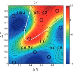
Figure 2 shows plots of two posterior emulator out-comes of the density difference field (Dd), given two different draws of 9 samples from a 10-member Stommel simulation set. The white contour line represents the true bimodal separation line between the two solutions of the dynamical simulator given a fully sampled system. The circles represent the outcomes from the simulator, the Stommel model, that is used to create the emulator. One of the circles is the 10th outcome, the validation point. It should fall within in the emulator space when the emulator is a reasonable representation of the sim-ulator. When the color matches the background field, then the excluded point fits the emulator. For Fig. 2a, the excluded point, located in the top-right portion of the
FIG. 2. (a) Emulator estimate of the density dif-ference (Dd) spatial structure; nine simulator points (black circles) and the point not included in emulator estimate (one filled colored circle; red dot in top right-hand corner) are shown. The color indicates the value of the design pointy. (b) As in (a), but the simulator point not used by the emulator is in the upper-left corner atDS50.10,DT50.82 (a filled blue circle; almost the same color as the emulator estimate). (c) As in (b), but with the110 additional simulator outcomes used to create the emulator (white circles; a total of 19 design points). The vari-ance of the outcome with contour lines at 0.2 in-crements (nondimensional; dashed lines) are shown. The variance or uncertainty is higher for the fields that used only nine simulator points, as in (a) and (b), in the emulator creation.
field at (DTandDS)5(0.9, 0.9), is some distance from the emulator estimate as intimated by its red color with
DI 5 0.46. This emulator fails one of diagnostics for a good emulator, that is, the values forf(x) should give a mean value forF(x) (a yellow–green color) that rep-resents a plausible value of outcomeY. In the second case (Fig. 2b), the emulation is more successful be-cause the excluded point (upper-left region, atDS,DT5
0.2, 0.8) falls within the emulator distribution. This em-ulator gives a reasonable estimate for a validation point (DI50.13).
Figures 2a,b also show that a large part of the simulator space is void of any sample points. The overlaid dashed contour lines (contour interval is 0.2) show the variance at any given point, and, thus, the uncertainty in its estimate. From the result of our 9-member ensemble emulation, we can further explore the initial condition space by sam-pling the region for values of DS between 0.4 and 1. Even if we did not know the underlying field ofDd out-comes, we might believe that with the strong gradient in the initial estimate of the Dd field, further sampling of the region with the gradient might be useful to refine the emulator. For our example, we resample using a simple scheme of choosing 10 addition points between 0.4 and 1 for theDS parameter and leaveDT to be sampled be-tween 1 and 0 again. Figure 2c is the resulting emulator density difference field using this expanded set of 19 simulator points. It is easily seen that the emulation outcomes space is much closer to the true spatial field of the simulator outcomesDd. (The validation point atDS,
DT50.2, 0.8 has aDIof close to 0.) The variance of the
emulated solution is also reduced in Fig. 2c with the ad-ditional simulator points. There is a shift in location of the region of high values. It is shifted so that it is more contained within the white contour that denotes the true division between the regimes. This is to be expected be-cause of the additional simulator points within that area are being used to create the revised emulator. In other words, a more accurate emulator is created because we have provided more local simulator information. This illustrates the use of a sequential design process to ex-plore regions of high uncertainty.
The sampling characteristics on an emulator solution can also be shown by usingn540 rather than 10. Using 39 of the 40 simulator outcomes, we created an emulator with its solution shown in Fig. 3a. It shows a much more realistic representation of the expected density space over all the possibleDTandDSvalues. The 40th point, not included in the emulator creation, is located at about (DS,DT) 5(0.18, 0.81) marked by an ‘‘x.’’ The black curve is the true curve that delineates the two stable so-lutions. Ideally, we would want the emulator solution of this delineation, represented by the white line, to lie on the truth, the black line. Figure 3b shows the same figure, but with the shaded areas greater than two standard de-viations of the solution. (The thin lines represent the variance.) As this figure shows, this emulator has pro-duced a region that is overconfident (i.e., the solution’s variance is smaller than the measured variance to in-dependent data) around the locationDS 50.4, DT 5
0.35–0.55, as well as underconfident (i.e., too much vari-ance) in the shaded areas with large spread about the
FIG. 3. (a) Emulator estimate of density difference (Dd) withn539 and one unused simulator outcome result; 39 points are denoted (black circles). The 0 contour (white contour line) and the step between two outcomes of the dynamical system (black contour) are shown. (b) As in (a), but only for thef(x) not within two standard deviations of the midpoint (shaded). Contour lines show the step between two outcomes of the dynamical system (thick black contour), and the relative variance (at 0.05 increments) for emulator estimates (thin black lines). (c)DIfor a set of 100 validation points with the points excluded fromDMDcalculation indicated (open circles). The step between the two outcomes of the dynamical system (contour line) is shown.DIis defined in section 2b.
black contour. We might also want to further sample the left side and bottom-right corner regions, because of their particularly high variance. In more realistic applications, even when the true solution is unknown, we still have an idea of the uncertainty (i.e., variance) of the emulator solution to help produce a more refined solution.
There are other methods that address highly nonlinear outcomes, such as methods that divide up the outcome space and emulate each subspace separately (Gramacy and Lee 2008). In general, these methods assume that the location of such separate spaces is known as our case; however, it is not always the case. Thus, we just limit our emulator illustration to the most general of situations.
Figure 3b can also be used to estimate the probability that this system will flip from one stable regime to an-other. For example, if we hadDS50.9 andDT50.35, we could give an estimate with an associated uncertainty that the system will flip if theDTvalue increases to 0.4. While this simulator and its emulator are straightfor-ward to understand, a system with more parameters and more complexity will add additional complications to-ward understanding such predictions. However, this type of methodology allows us to explore the space in a sys-tematic manner. TheDIvalues for a set of 100 validations are shown in Fig. 3c, along with the black contour line separating the two states of the simulator. It is clear that the points that have the least skill (values ofDIgreater than62) are in the region where the jump between the two states occurs. We would expect such a result, given the extreme nature of the nonlinearity. This can be quantified also using theDMDdiagnostic. When using all of the 100 validation points,DMD’10 000. If we remove from the calculation the points with the greatest uncer-tainty (DI. 62), thenDMD592.8 for this set of 81 points. This is what we would expect theDMDdiagnostic to be for a reasonable emulation (see section 2b; Bastos and O’Hagan 2009).
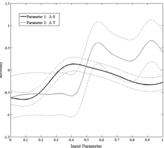
Last, we show the sensitivity of the solution (Dd) to each of the input parameters (DTandDS) in Fig. 4. The figure shows the integrated response of the emulator for each of the parameters across the space of the other parameter. Figure 4 explicitly illustrates the division between the influence of the initial conditions of the temperature and salinity differences on the outcome. It shows the response of one of the two inputs, given the other input is held constant at 0.5. ForDT, the important shift is between 0.2 and 0.3, while the salinity shift is between 0.4 and 0.5. Again, while these relationships can be easily seen with the simulator without the emu-lator, the plot is shown to illustrate how input parame-ters relate to one another and how one can determine the importance of one variable over another and the interaction between the multiple variables.
4. An example using the GENIE-1 simulator
In the second, more complex example, we use a set of simulator outcomes that have been previously created (Challenor et al. 2010) to illustrate the methodology when we have a more complex simulator that still has highly nonlinear behavior.
The GENIE-1 simulator, also known as the C-GOLDSTEIN model, is a coupled climate model of intermediate complexity. It has reduced physics for the three-dimensional ocean, which is coupled to a two-dimensional energy–moisture balance model. Challenor et al. (2010), Marsh et al. (2004), and Edwards and Marsh (2005) describe the simulator in detail. The ver-sion of GENIE used in this paper has 64 longitudes and 32 latitudes, which are uniform in the longitude and sin (latitude) coordinates, giving boxes of equal area in physical space. There are eight depth levels in the ocean on an uniformly logarithmically stretched grid, so that the box depth increases from 175 to 1420 m. GENIE-1 is deterministic. To remove dependence on initial condi-tions the simulator was spun up for 4000 yr to the year 2000; the last 200 yr of the run had historic CO2forcing
applied. The outcome is the maximum of the meridi-onal overturning circulation (MOC) in the Atlantic Ocean. The time evolution of these outcomes is shown in Fig. 5a, showing at least two distinctive end states. The majority of the model runs have strength of the meridional overturning in the range of 10–70 Sv (1 Sv[ 106m3s21), but there are a number runs where the overturning circulation has completely collapsed and
FIG. 4. The sensitivity of the outcome metric, the density dif-ference (Dd), to the input parameters (DSandDT). The sensitivity is the integrated response of one parameter across the parameter space of the other, as seen by the emulator.
there is zero overturning at the end of the run. The former correspond to an active MOC at year 2000 while the latter correspond to circulation where the overturning had collapsed several thousand years ago. There is a sugges-tion that the former set is, in fact, two sets because some cases show that increasing the CO2causes a decrease in
the strength of the overturning while in others it in-creases. In terms of the final strength of the MOC, how-ever, we can only distinguish two states: MOC on and off. Marsh et al. (2004) did an exhaustive evaluation (many thousands of runs) for two input parameters (atmo-spheric diffusion and Atlantic–Pacific moisture flux) by leveraging a large number of personal computers (via grid technology) in a similar (but not exactly the same) simulator. They showed that, like the Stommel model, there is bistability in the maximum overturning, although the nonlinearity is not as extreme as in the Stommel model.
Using the methods described earlier we built an em-ulator for the ensemble of overturning outcomes at year 2000. When we fix all of the parameters, apart from the atmospheric diffusion and Atlantic–Pacific moisture flux, to values similar to those in Marsh et al. (2004) we pro-duce figures similar to their Fig. 4 from our emulator. This is shown in Fig. 5b. For our first example we illustrated the emulator with plots of the mean and variance. Emu-lators, though, are more than simply a mean function and an associated variance; they are statistical distributions of
functions. We illustrate this with two such functions in Fig. 5b. These are random draws from the emulator, setting 14 parameters to be constant and only varying 2: the atmospheric diffusion and the Atlantic–Pacific mois-ture flux. The dots/circles are the outcomes for the 96 simulator points at the given input parameter values. If the emulator is properly representing the GENIE model, then theDIwill have a Student’sttest distribution with the degrees of freedom equal to the number of runs in the training set (Bastos and O’Hagan 2009), which in our case is 95 (i.e., 96 runs, with the run being tested being held back). This is approximately a normal distribution. The
DIvalue is within the expected 95% uncertainty bounds (61.96) for the black dots (the location is withheld from the emulator training set and used as a validation point). The six black circles are points that fail the DI criteria when withheld. With 96 points we would expect about 5 to be outside 95% confidence intervals, so 6 is not an unreasonable number, and the emulator validates. The nonlinear behavior of the emulator is consistent with the findings of Marsh et al. (2004). Despite only having a very small number of runs (96 over 16 dimensions) the emu-lator is able to reproduce the nonlinear behavior.
5. Conclusions
The test problems illustrate how emulators can be useful to explore aspects of complex geophysical
FIG. 5. (a) The time evolution of the MOC metric over 4000 yr of the GENIE-1 model spin up. Each run with a different set of input values for the 16 parameters are shown (gray lines). Note: there are two sets of end points. The majority of the runs have a final MOC value between 10 and 70 SV. There is a second set where the final MOC is near zero. These correspond to an active and collapsed MOC, respectively. (b) Two possible outcome surfaces created by the emulator with respect to the parameters: atmospheric diffusion and Atlantic–Pacific moisture flux. The MOC values from the 96 simulations given the input values for these two parameters at year 2000 are shown (black dots). The simulator or design input locations are shown: points that produce acceptableDIvalues, when withheld from the design (one at a time; black dots), and those that are locations that have unacceptableDIvalues (black circles). Note there are a small number of points that are at 0, but these are obscured by the projection.
simulators when the resources are not available to run thousands of simulations with the following points: 1) We have shown how emulators can be built and used
to explore the parameter space of two nonlinear geophysical simulators. The first example is an ex-treme illustration, in that most systems will not have distinct bimodal regimes, but rather more continuous solutions that have less stringent fitting requirements. The second example shows the method as applied to a more complex problem. These two examples are used because they are not so complex and com-putationally expensive that we cannot compare the emulator solution to a comparable very large simula-tor ensemble for the same simulasimula-tor. In the case of AOGCMs, the computational intensity of these sim-ulators prohibits the creation of very large (order 10 000) ensembles. This is the reason why we might consider the use of an emulator to explore a simula-tor’s parameter space, as well as why such simulators cannot be used to illustrate an emulator’s intrinsic capabilities. The size of the ensemble needed to build the training and validation sets for an emulator is usually possible even with large AOGCMs, whereas Monte Carlo calculations are beyond reach for even relatively small simulators. Marsh et al. (2004) went to extreme lengths to find enough computational re-sources to study the properties of GENIE, a relatively simple coupled climate simulator, for only two inputs. 2) If we know a priori that our simulator was highly nonlinear and we had some information on the form of the nonlinearity, we could attempt to model the nonlinearity directly. One way would be to build a prior mean function that could include steps. Alter-natively, treed Gaussian processes (Gramacy and Lee 2008) could possibly be used. These split the input space into a number of regions and fit separate GP’s in each region. Both of these approaches have difficul-ties. Finding a suitable form for the mean function to encapsulate the nonlinear behavior is nontrivial, while treed Gaussian processes are computationally expen-sive. Our results show that for even highly nonlinear simulators, the additional expense is not necessary. 3) To build an emulator we make a number of
assump-tions. The main one is that the simulator is smooth. We have shown here that even if this assumption is violated, the resulting emulator is still a good ap-proximation to the full simulator.
4) These emulators, thus, should prove useful to explore the full space of complex simulations (AOGCMs), including its parameter space, initial conditions, and/ or boundary conditions. AOGCMs, especially in the context of climate projections or seasonal forecasts,
would benefit from such an exploration of their full parameter space through the use of emulators. In the past, such methods have not been used to look at AOGCMs because of the high computational costs. However, now that computational speeds and re-sources have increased to the point that such simula-tor/emulator problems can be explored, initial efforts are moving forward.
Acknowledgments. David Stevens prompted us to justify that emulators can be used in either bimodal or bifurcation-type problems. We thank the Isaac Newton Institute of Mathematical Sciences at the University of Cambridge for allowing us to spend time at the institute where this research was completed. J. Rougier provided helpful comments for improving the manuscript. This work was also completed with funding under NSF Grant 0851065. Jim Price is thanked for making his Stommel (1961) model Matlab code (public domain software) available. We thank Doug McNeal for the GENIE data used in the second example. We also thank two anony-mous reviewers for their time and helpful suggestions.
APPENDIX
Stommel Model Details
The Stommel model equations for the time evolution of temperature and salinity for the system are as follows:
›T
›t 5c(T*2T)2j2qjT, (A1)
›S
›t 5b(S*2S)2j2qjS, (A2)
wherecandbare coefficients andqis a flux or flushing rate between two basins;T* andS* are fixed reference temperature and salinity values; andT andSare tem-perature and salinity values that vary over time.
Further,q can be defined as the difference in the density of the two vessels times a resistance 1/k, such thatkq5r12r2, whereris given by a simple equation
of stater5r0(12aT 1bS). Here,aandbare
un-defined coefficients in the dimensional case (see the nondimensional definition of Rbelow). If we define various quantities in nondimensional terms such that
f52q/c,t5ct,d5(b/c),y5(T/T*), and x5(S/S*), then we can rewrite the equations in nondimensional terms as
›y
›x
›t5d(12x)2jfjx. (A4)
Now let us define the temperatures and salinities for r1andr2such thatT5T15 2T2andS5S15 2S2for
the two boxes, and a terml5(c/(4roaT*))k. In doing
so, we find the third equation, which defines the density difference in nondimensional terms,
Dd5lf5(2y1Rx) , (A5) whereR5(bS*/aT*).
Substituting (A5) into (A4) and (A3), we get our final equations that define our model in nondimensional terms, ›y ›t512y2 y ljRx2yj, (A6) ›x ›t5d(12x)2 x ljRx2yj. (A7)
For our test emulator problem, we set the values ofl,
R, andd(R52,l50.2, andd51/
6). In section 3, we use DSto refer toxandDTto refer toy, because the main text usesxfor another purpose and in this appendix we wanted to be consistent with Stommel (1961).
We use the simulator (the Stommel model) in the following way: we create an ensemble of initial values for x and y (e.g., Latin hypercube sampling over all possible values) for nruns, and run the simulator for-ward in time until stable for eachn, generating an en-semble of outcomesDd. The emulator is created using the knowledge of how the set ofDdoutcomes are asso-ciated to thexandyinput values.
REFERENCES
Bastos, L., and A. O’Hagan, 2009: Diagnostics for Gaussian pro-cess emulators.Technometrics,51,425–438.
Bayarri, M. J., J. O. Berger, R. Paulo, J. Sacks, J. A. Cafeo, J. Cavendish, C.-H. Lin, and J. Tu, 2007: A framework for validation of computer models.Technometrics,49,138–154, doi:10.1198/004017007000000092.
Berliner, L. M., R. F. Milliff, and C. K. Wikle, 2003: Bayesian hi-erarchical modeling of air-sea interaction.J. Geophys. Res., 108,3104, doi:10.1029/2002JC001413.
Challenor, P., 2011: Designing a computer experiment that in-volves switches.J. Stat. Theory Pract.,5,47–57.
——, R. Hankin, and R. Marsh, 2006: Towards the probability of rapid climate change.Avoiding Dangerous Climate Change,
H. Schellnhuber et al., Eds., Cambridge University Press, 55–63. ——, D. McNeall, and J. Gattiker, 2010: Assessing the probability of rare climate events. The Oxford Handbook of Applied Bayesian Analysis,T. O’Hagan and M. West, Eds., Oxford University Press, 403–430.
Clark, J., 2005: Why environmental scientists are becoming Bayesians.
Ecol. Lett.,8,2–14.
Edwards, N. R., and R. Marsh, 2005: Uncertainties due to trans-port-parameter sensitivity in an efficient 3-D ocean-climate model.Climate Dyn.,24,415–433.
Frolov, S., A. Baptista, T. Leen, Z. Lu, and R. Merwe, 2009: Fast data assimilation using a nonlinear Kalman filter and a model surrogate: An application to the Columbia River estuary.Dyn. Atmos. Oceans,48,16–45.
Gramacy, R. B., and H. K. Lee, 2008: Bayesian treed Gaussian process models with an application to computer model-ing. J. Amer. Stat. Assoc., 103, 1119–1130, doi:10.1198/ 016214508000000689.
Habib, S., K. Heitmann, D. Higdon, C. Nakhleh, and B. Williams, 2007: Cosmic calibration: Constraints from the matter power spectrum and the cosmic microwave background.Phys. Rev., 76D,083503, doi:10.1103/PhysRevD.76.083503.
Higdon, D., M. Kennedy, J. Cavendish, J. Cafeo, and R. Ryne, 2004: Combining field observations and simulations for cali-bration and prediction.SIAM J. Sci. Comput.,26,448–466. Holden, P. B., and N. R. Edwards, 2010: Dimensionally reduced
emulation of an AOGCM for application to integrated assess-ment modelling.Geophys. Res. Lett.,37,L21707, doi:10.1029/ 2010GL045137.
Leslie, W. G., A. R. Robinson, P. J. J. Haley, O. Logutov, P. A. Moreno, P. F. J. Lermusiaux, and E. Coelho, 2008: Verification and training of real-time forecasting of multi-scale ocean dy-namics for maritime rapid environmental assessment.J. Mar. Syst.,69,3–16.
Loeppky, J. L., J. Sacks, and W. J. Welch, 2009: Choosing the sample size of a computer experiment: A practical guide.
Technometrics,5,366–376, doi:10.1198/TECH.2009.08040. Logemann, K., J. O. Backhaus, and I. H. Harms, 2004: SNAC:
A statistical emulator of the north-east Atlantic circulation.
Ocean Modell.,7(1–2), 97–110.
Marsh, R., and Coauthors, 2004: Bistability of the thermohaline circulation identified through comprehensive 2-parameter sweeps of an efficient climate model.Climate Dyn.,23,761– 777.
McKay, M. D., R. J. Beckman, and W. J. Conover, 1979: A com-parison of three methods for selecting values of input variables in the analysis of output from a computer code.Technometrics, 21,239–245.
Murphy, J. M., D. Sexton, D. Barnett, G. Jones, M. Webb, M. Collins, and D. Stainforth, 2004: Quantification of model-ling uncertainties in a large ensemble of climate change sim-ulations.Nature,432,768–772.
Oakley, J., and A. O’Hagan, 2004: Probabilistic sensitivity analysis of complex models: A Bayesian approach.J. Roy. Stat. Soc., 66B,751–769.
O’Hagan, A., 2006: Bayesian analysis of computer code outputs: A tutorial.Reliab. Eng. Syst. Saf.,91,1920–1300.
——, and J. Forster, 2004:Bayesian Inference. Vol. 2B,Kendall’s Advanced Theory of Statistics,Arnold, 480 pp.
——, C. E. Buck, A. Daneshkhah, J. R. Eiser, P. H. Garthwaite, D. J. Jenkinson, J. E. Oakley, and T. Rakow, 2006:Uncertain Judgments: Eliciting Experts’ Probabilities. Wiley, 338 pp. Rasmussen, C., and C. Williams, 2006: Gaussian Processes for
Machine Learning. MIT Press, 266 pp.
Rougier, J., and D. Sexton, 2007: Inference in ensemble experi-ments.Philos. Trans. Roy. Soc. London,A365,2133–2143. Sanso´, B., and C. Forest, 2009: Statistical calibration of climate
system properties.J. Roy. Stat. Soc.,58,485–503.
——, ——, and D. Zantedeschi, 2008: Inferring climate system properties using a computer model.Bayesian Anal.,3,1–38.
Sapsis, T. P., and P. F. J. Lermusiaux, 2009: Dynamically orthog-onal field equations for continuous stochastic dynamical sys-tems.Physica D,238,2347–2360.
Sobol, I., 1967: Distribution of points in a cube and approximate evaluation of integrals.U.S.S.R. Comput. Math. Math. Phys., 7,86–112.
Stommel, H., 1961: Thermohaline convection with two stable re-gimes of flow.Tellus,13,224–230.
Strounine, K., S. Kravtsov, D. Kondrashov, and M. Ghil, 2010: Reduced models of atmospheric low-frequency variability: Parameter estimation and comparative performance.Physica D,239,145–166.
Urban, N. M., and T. E. Fricker, 2010: A comparison of Latin hypercube and grid ensemble designs for the multivariate emulation of an Earth system model.Comput. Geosci.,36,
746–755, doi:10.1016/j.cageo.2009.11.004.
van der Merwe, R., T. K. Leen, Z. Lu, S. Frolov, and A. M. Baptista, 2007: Fast neural network surrogates for very high dimensional physics-based models in computational oceanography.Neural Networks,20,462–478.
Williams, B., D. Higdon, J. Gattiker, L. Moore, M. McKay, and S. Keller-McNulty, 2006: Combining experimental data and computer simulations, with an application to flyer plate ex-periments.J. Bayesian Anal.,4,765–692.