University of Wollongong University of Wollongong
Research Online
Research Online
Faculty of Engineering and Information
Sciences - Papers: Part B Faculty of Engineering and Information Sciences 2018
Spatial data compression via adaptive dispersion clustering
Spatial data compression via adaptive dispersion clustering
Yuliya MarchettiCalifornia Institute of Technology Hai Nguyen
California Institute of Technology Amy Braverman
California Institute of Technology, [email protected] Noel A. Cressie
University of Wollongong, California Institute of Technology, [email protected]
Follow this and additional works at: https://ro.uow.edu.au/eispapers1
Part of the Engineering Commons, and the Science and Technology Studies Commons
Recommended Citation Recommended Citation
Marchetti, Yuliya; Nguyen, Hai; Braverman, Amy; and Cressie, Noel A., "Spatial data compression via adaptive dispersion clustering" (2018). Faculty of Engineering and Information Sciences - Papers: Part B. 1992.
https://ro.uow.edu.au/eispapers1/1992
Spatial data compression via adaptive dispersion clustering
Spatial data compression via adaptive dispersion clustering
AbstractAbstract
Spatial Dispersion Clustering (ASDC), a new method of spatial data compression, is specifically designed to reduce the size of a spatial dataset in order to facilitate subsequent spatial prediction. Unlike traditional data and image compression methods, the goal of ASDC is to create a new dataset that will be used as input into spatial-prediction methods, such as traditional kriging or Fixed Rank Kriging, where using the full dataset may be computationally infeasible. ASDC can be classified as a lossy compression method and is based on spectral clustering. It aims to produce contiguous spatial clusters and to preserve the spatial-correlation structure of the data so that the loss of predictive information is minimal. An extensive simulation study demonstrates the predictive performance of these adaptively compressed datasets for several scenarios. ASDC is compared to two other data-reduction schemes, one using local
neighborhoods and one using simple binning. An application to remotely sensed sea-surface-temperature data is also presented, and computational costs are discussed.
Disciplines Disciplines
Engineering | Science and Technology Studies Publication Details
Publication Details
Marchetti, Y., Nguyen, H., Braverman, A. & Cressie, N. (2018). Spatial data compression via adaptive dispersion clustering. Computational Statistics and Data Analysis, 117 138-153.
Spatial data compression via adaptive dispersion clustering
Yuliya Marchettia,∗, Hai Nguyena, Amy Bravermana, Noel Cressieb,a
aJet Propulsion Laboratory, Pasadena, CA, USA bUniversity of Wollongong, Wollongong, Australia
Abstract
In this article, we introduce a method of spatial data compression, which we call Adaptive Spatial Dispersion Clustering (ASDC). It is specifically designed to reduce the size of a spatial dataset in order to facilitate subsequent spatial prediction. Unlike with traditional data and image compression methods, the goal of ASDC is to create a new dataset that will be used as input into spatial prediction methods, such as traditional kriging or Fixed Rank Kriging, where using the full dataset may be computationally infeasible. ASDC can be clas-sified as a lossy compression method and is based on spectral clustering. It aims to produce contiguous spatial clusters and to preserve the spatial correlation structure of the data so that the loss of predictive information is minimal. Through simulations, we demonstrate the predictive performance of these adaptively compressed datasets for several scenarios. ASDC is compared to two other data-reduction schemes, one using local neighborhoods and one using simple binning. We also present an application to remotely sensed sea-surface temperature data.
Keywords: spatial data compression, spectral clustering, spatial clusters, spatial dispersion function
1. Introduction
Very large spatial and spatio-temporal datasets are becoming more commonplace in social, commercial, and scientific research. In the social and commercial realms this is largely due to the expansion of the internet, and the computerization of many aspects of daily life. In science, new technologies for data collection and experimentation have led to the demand for new analysis methods specifically designed for new data types. One area where this is
∗Corresponding author
Email addresses: [email protected](Yuliya Marchetti),[email protected]
especially true is Earth Science, where satellite remote sensing data play an increasingly important role in understanding the physics of the Earth’s system and interactions among its components. Remote sensing data can be massive, with hundreds of millions to billions of data points collected per day, but at the same time they can be sparse, with gaps in coverage due to orbit patterns and observing technology limitations.
Spatial and spatio-temporal statistical inference methods are key to obtaining maximum scientific return from these data, but massiveness poses a serious challenge to conventional spatial statistical modeling approaches. It is natural to look for ways to make the compu-tations more efficient, and various methods based on simplification of the statistical model have been proposed. Some enforce sparsity on large spatial covariance matrices (Furrer et al., 2006;Kaufman et al., 2008) or precision matrices (Besag and Kooperberg,1995; Rue and Held, 2005;Lindgren et al.,2011; Eidsvik et al.,2014; Datta et al.,2015;Gramacy and Apley,2015;Nychka et al.,2015), and others use dimension reduction to reduce the number of parameters required to specify covariance (Banerjee et al.,2008;Cressie and Johannesson, 2008; Finley et al., 2009; Sang and Huang, 2012; Nguyen et al., 2012). However, with ever-increasing data collection capabilities, the majority of these methods by themselves may not be enough because they still require holding large matrices, e.g., basis-function matrices, in memory. The method presented in this article, Adaptive Spatial Dispersion Clustering (ASDC), takes a different approach that is intended to complement dimension-reduction and sparse methods: make the data smaller in a way that preserves the essential information required for good spatial prediction.
The idea of making data smaller while preserving their essential characteristics is not new. When a spatial dataset is massive, such as is the case for high-resolution global remote sensing data, spatial prediction could be performed by limiting the data to a small region of interest, and ignoring the rest. In fact, local kriging (Haas, 1990; Cressie, 1993; Hammerling et al.,2012) and similar methods rely on such an approach. An alternative is to use compressed data instead, where compression here means that the data outside the region of interest have been aggregated to coarse resolution. This approach could be advantageous if aggregation is done in a way that preserves spatial information and produces globally valid spatial covariance structures. “Gridding” or “binning,” in which the entire spatial field is aggregated to a coarse spatial resolution, is a form of naive data reduction that does not explicitly address the preservation of spatial covariance.
Clustering is a foundation of traditional data compression, but spatial dependence is usually not incorporated directly into the fidelity criterion. In the case of image
sion, there are approaches that do account for spatial dependencies and cluster coherence (Ambroise et al.,1997;Hu and Sung,2006;Craddock et al.,2012), but the goal is to recreate an approximation that is visually indistinguishable from the original image, rather than to preserve spatial structure for purposes of inference per se. In contrast, ASDC explicitly incorporates key aspects of spatial covariance through the use of spatial dispersion functions (Sampson and Guttorp, 1992). For spatial predictions in a region of interest, data outside the region of interest are compressed by assigning the geographic locations associated with them to spatial clusters. Each spatial cluster is represented by the mean value of the data at its constituent locations. Cluster assignments are obtained by applying spectral clustering to a weighted similarity matrix that accounts for covariances among locations outside the region of interest, and covariances between locations inside and outside. This forces spatial contiguity, and causes clusters near the region of interest to be smaller than those far away because spatial covariance generally decreases with distance. In this paper, we demonstrate our method using simulated and real data of moderate size, rather then massive size, as a proof-of-concept.
The remainder of this paper is organized as follows. In Section2we provide an overview of and motivation for spatial data compression. We describe the ASDC algorithm and the set of concepts necessary to understand and explain its logic. In Section 3 we describe a simulation experiment that quantifies ASDC’s performance versus local kriging and binning by comparing these three methods on synthetic data where the true spatial covariance function is known. Then, in Section 4, we apply the three methods to a relatively small sea-surface temperature dataset for which the true spatial covariance function is not known. This demonstrates the practical value of ASDC in real-world situations. Finally, Section 5 offers some conclusions, a discussion of computational challenges, and directions for future research.
2. Methods
Most methodologies applied to spatial data operate on the principle of the First Law of Geography (Tobler, 1970): locations that are closer to each other tend to behave more similarly than do those further apart. This implies that spatial covariance decays with geographic distance in a more or less continuous way. In other words, data from locations far away from a point or region of interest carry less information about the behavior of the process at the locations of interest than do data obtained at nearby sites. Consequently, compressing data from far away should have less affect on the precision and accuracy of
optimal spatial predictors such as kriging predictors. In this section we formalize these ideas and describe how the ASDC algorithm combines them to provide a formal approach to spatial data compression.
2.1. Framework
Let {Y(v) : v ∈ D ⊂ D ⊂¯ R2} be a hidden, real-valued process of interest on a
two-dimensional spatial domain, whereD={v1, . . . ,vN},N is the size ofD, and ¯Dis the union
of basic areal units (BAUs). FollowingNguyen et al.(2012), a BAU is a fine-scale spatial tile that represents the support of the smallest area for which inferences will be made. The entire spatial domain ¯D is tesselated into a set of these non-overlapping tiles: ¯D =SN
k=1Ak, and
each BAU Ak is uniquely identified with a spatial location, vk. Henceforth, when referring
to a location vk, it is to be understood that we are referring to its corresponding BAU Ak
and vice versa.
Let Z(s) be an observation at location s, and assume that Z(s) is the sum of the true spatial process,Y(s), and measurement error, (s):
Z(s) =Y(s) +(s); s∈ D, (1)
where (·) is a mean-zero white-noise Gaussian process with variance, var((·)) =σ2 .
Sup-pose that data are observed at {s1, . . . ,sn} ⊂ D, and define the vector of observations as
Z = (Z(s1), . . . , Z(sn))T, where n ≤ N. We are typically interested in inferring Y(v0) at a
new location v0 ∈ D by minimizing the mean squared prediction error (MSPE):
M SP EY(v0),Yˆ(v0) =E Y(v0)−Yˆ(v0) 2 ,
with respect to ˆY(v0). In the case of kriging, ˆY(v0) = aTZ is a linear predictor of Y(v0)
based on all the available observations Z, and we wish to minimize the MSPE with respect to a ∈ Rn. The optimal weights, a, are called kriging weights, which can be obtained by
solving linear systems for each prediction location (e.g., Cressie, 1993). These are based on the covariance matrixC= (cij)n×n, wherecij = cov (Z(si), Z(sj)), and on cov(Y(v0), Z(si)).
Sincen can be very, very large, it may not be feasible to compute ausing all the data. Yet, it is still desirable to use as much of the dataset’s information as possible, and rather than simply ignoring a portion of the elements of Z, we will reduce its size with spatial data compression.
For the sake of realism, consider a block of prediction locations, D0 = {v0,1, . . . ,v0,M}
of size |D0| = M. Then the rest of the locations form an exterior subdomain De = D \ D0. The observed data vector Z can then be partitioned as Z = ZT0,ZTe
T , where Z0 = (Z(s1), . . . , Z(sm)) T and Ze = (Z(sm+1), . . . , Z(sn)) T
, and where {s1, . . . ,sm} ∈ D0 and {sm+1, . . . ,sn} ∈ De. We assume that the region of interest can always be chosen such that D0∩ {s1, . . . ,sn} 6=∅, i.e. there is always at least one observed location.
Our goal is to perform spatial compression by clustering N −M locations in De into K
disjoint subsets, Γe,j, with ∪Kj=1Γe,j = De and where K n and is currently pre-specified
by the user based on memory and other computational limitations. We then assign the
`-th location in D0 to a (K +`)-th cluster, ΓK+` = v0,`, such that ∪M`=1ΓK+` ∪Γe = D.
We compute the aggregated data, Ψ= (ψ(Γ1), . . . , ψ(ΓK+M))T from Z; see (3) below. The
subsequent statistical inference forD0 based on Ψ should be “similar” to that based on Z.
A compression matrix is an N×(K+M) binary matrix Qin which thek-th row corre-sponds to thek-th location inD,k = 1, . . . , N, and thej-th entry in that row corresponds to thej-th spatial cluster, Γj,j = 1, . . . , K+M. Thek, j-th cell ofQ, denoted by [Q]kj, is 1 if
thek-th location is assigned to Γj and is 0 otherwise, with the proviso thatPKj=1+M[Q]kj = 1.
The j-th spatial cluster is defined by
Γj = N
[
k=1
{vk : [Q]kj = 1}, (2)
and it is natural to define the spatial support of Γj as the union of the spatial supports
associated with its constituent locations: the support of Γj is ∪Nk=1{Ak : [Q]kj = 1}.
Finally, ψ(Γj) = 1 nj n X i=1 Z(si)1(si ∈Γj), nj >0, (3)
denotes the aggregated data for the j-th cluster; j = 1, . . . , K +M. In (3), 1(·) is the indicator function and nj =Pni=11(si ∈Γj). An aggregated value does not exist if nj = 0
(i.e. if there are no observations associated with thej-th cluster Γj).
Kriging using the available dataZinDwould result in the full-kriging predictor, ˆY(v0) =
aT
0Z, forv0 ∈ D0. Alternatively, the compressed kriging predictor is ˜Y(v0) = bT0Ψ. Ideally,
they give similar predictions. That is, ideally,
M SP EYˆ(v0),Y˜(v0) =E ˆ Y(v0)−Y˜(v0) 2 =Eh aT0Z−bT0Ψ2i≈0, (4)
but the cost of computing bT
0Ψ is substantially less than that of aT0Z. Since ˆY(v0) is the
best linear unbiased predictor, and ˜Y(v0) is linear in Ψand hence in Z, and it is unbiased,
then Eh aT
0Z−bT0Ψ
2i
≥0.
2.2. Spatial dispersion function
The central idea behind ASDC is to use the spatial dispersion function to perform spatial clustering in De; that is, we specify Q in a way that the left-hand side of (4) is as small as
possible. The spatial dispersion function is a smooth, non-negative function of geographic locations that indicates the spatial covariance structure of these locations (Sampson and Guttorp, 1992). Except for smoothness and non-negativity, we do not impose any other constraints on the spatial dispersion function and so, likeSampson and Guttorp (1992), we avoid using the term variogram. We exploit the spatial dispersion function to enforce fidelity to the underlying spatial covariance function, to induce spatial contiguity, and to adaptively determine the appropriate degree of compression throughout the spatial subdomain De.
A measure of local spatial dispersion between any two locations si andsj is the squared
difference between the corresponding observed values Z(si) and Z(sj):
d2ij =|Z(si)−Z(sj)|2. (5)
Define the spatial dispersion function gφ(·) as a smooth continuous function of distance
between si and sj, D(si,sj), that depends on the spatial variability of Z expressed through
parameters φ. For example, D(si,sj) = ksi−sjk, but other distances, such as great circle
distance on the spheres are possible. The spatial dispersion function gφ can assume any
form as long as it is a smooth and non-negative function of distance. For example, it can be a specific parametric form used in spatial statistics or it can be a non-parametrically estimated function, such as a non-negative spline (Wever, 1988; Papp and Alizadeh, 2014). Like a variogram, the spatial dispersion function,gφ, can be fitted by minimizing
X
i
X
j
|d2ij −gφ(D(si,sj))|2, (6)
with respect toφ. This results in ˆφ and the fittedgφˆ; see Sampson and Guttorp (1992) and
Bornn et al.(2012), where spatial dispersion functions are used in optimal spatial estimation problems to construct covariance matrices forZ. Here, we use the spatial dispersion function to inform spatial data compression and not directly for estimation or prediction.
Ultimately, we will determine the compression matrixQby applying a spectral clustering 6
algorithm to a collection of N −M feature vectors, each representing one of the N −M
locations inDe. Section 2.4 explains how we derive the features and use them to populate a
similarity matrix that is input into the clustering algorithm, but first we review the basics of spectral clustering in Section 2.3 below.
2.3. Spectral clustering
Spectral clustering (Shi and Malik, 2000; Ng et al., 2002) is a very popular method in unsupervised learning because of its simplicity and superior performance (Von Luxburg, 2007). Spectral clustering does not make any assumptions about the shape or structure of the resulting clusters, it captures non-spherical and non-convex clusters well, and it can also be applied to very large datasets (Chen et al.,2011;Song et al.,2008;Zare et al.,2010). See Von Luxburg(2007) for a summary of spectral clustering and a discussion of its relationship to spectral graph theory and graph partitioning problems.
We briefly outline the underlying methodology of spectral clustering. Let x1, . . . ,xn be
a set of data vectors, and for i= 1, . . . , n, let wij represent a “similarity” measure between
xi and xj, where wij ≥ 0, wij = wji. The goal of spectral clustering is to group the data
vectors x1, . . . ,xn into K subsets using weights wij such that data points within a subset
are “similar” to each other, while data points in different subsets are “dissimilar”. There are many options for calculating the similarity weights wij. For example, wij can simply take
values ∈ {0,1}, with wij = 0 if the two data vectors xi and xj are not related and wij = 1,
if they are. The most commonly used weights are computed based on the Gaussian kernel:
wij = exp −kxi−xjk2/2τ2
, i, j = 1, . . . , n, (7)
where τ2 is called the scaling parameter and is usually defined by the user. The weights
wij are collected in a weighted similarity matrix W = [wij]n×n, from which a normalized
Laplacian matrix, L, is computed:
L=I−D−1/2WD−1/2, (8)
where D is diagonal with the ith diagonal element,dii, equal to the row sums of W, and I
is the identity matrix. That is,
wi+ = n
X
j=1
It is apparent from Equation (8) that L is an n×n square matrix containing normalized
dissimilarities.
The eigen-decomposition of L is given by,
L =QT ΛQ, (10)
whereQis then×nmatrix with columns that are the eigenvectors ofL, andΛis a diagonal matrix with the eigenvalues of L on the diagonal. Denote the columns of Q by q1, . . . ,qn
and the eigenvalues by λ1, . . . , λn. Assume that the eigenvalues are ordered from smallest
to largest, 0 = λ1 ≤ λ2 ≤ λn (Chung, 1997), and that columns of Q are in corresponding
order so thatQ= [q1, . . . ,qn]. The truncated n×K matrix of eigenvectors is,
U= [q1, . . . ,qK], (11)
whereK is the number of clusters.
The final step of spectral clustering is to apply the K-means clustering algorithm ( Har-tigan and Wong,1979;Arthur and Vassilvitskii,2007) to therows ofU. Since the rows ofU
correspond to x1, . . . ,xn, the result is an assignment of each xi to one of K clusters on the
basis of the similarities of xi to one another in a space that emphasizes specific aspects of
their relationships through W. In the next section, we describe how we use this to cluster
N −M locations in De in a way that respects the spatial covariance characteristics in De
for spatial compression as well as that between De and D0, as defined in Section 2.1. 2.4. Adaptive spatial dispersion clustering
To make good predictions at locations in D0 from locations in De, it is necessary to
pre-serve the covariance structure of the process betweenD0 and{ve,i ∈ De :i= 1, . . . , N −M}.
To adaptively compress locations inDe, it is also important to preserve the covariance
struc-ture of the process among all pairs of locations ve,i and ve,j, i, j = 1, . . . , N −M. The
weighted similarity matrix W discussed in Section 2.3 must incorporate both these covari-ance structures, and we achieve that by basing the weighted similarities on a combination of two different spatial dispersion functions that capture the two covariance structures.
To quantify spatial covariance structure among locations in De and between locations
in D0 and in De, we compute two sets of spatial dispersions as per (5): {d2e,ij = (Z(se,i)−
Z(se,j))2 : se,i,se,j ∈ De} are spatial dispersions between locations in De and {d20,`k =
(Z(s0,`)−Z(se,k))2 : s0,` ∈ D0,se,k ∈ De} are spatial dispersions between D0 and locations
in De. Using (6) we estimate two spatial dispersion functions, gφˆe from
d2e,ij and gφ0ˆ
fromd2
0,`k . The appropriate parametric forms of gφe and gφ0 are problem-specific; in our
applications, we have used both the exponential function and non-negative splines. The weighted similarities for spectral clustering we use are defined by
wij = exp −khe,i−he,jk 2 2√h0,i· √ h0,j , (12)
where he,i and he,j are (N −M)-dimensional vectors derived from the spatial dispersion
functiongφˆe that models the spatial structure inDe, andh0,iandh0,j are scalars derived from
the spatial dispersion function gφ0ˆ that models the relationship between locations ve,i ∈ De
and D0. Equation (12) is immediately recognizable as a form of the Gaussian kernel given
by (7) with xi and xj replaced by he,i and he,j, and τ2 replaced by
√ h0,i· √ h0,j . Next, we explain the derivations ofhe,i, he,j, h0,i, andh0,j.
Define the matrix Hfor which the ij-th element is
[H]ij =gφˆe(D(ve,i,ve,j)), (13)
fori, j = 1, . . . , N−M, where D(ve,i,ve,j) is a distance measure betweenve,i and ve,j. The
i-th row of H is a (N −M)-dimensional vector of spatial dispersions between location ve,i
and all other locations in De. Thus, row i of of H can be thought of as a basis expansion
that encodes the available information about how the process at ve,i covaries with all other
locations in De. In (12), he,i and he,j are obtained from the i-th and j-th rows of H,
respectively.
Define the geographic distance between location ve,i and D0 to be the distance between
ve,i and the location inD0 that is nearest to ve,i:
D(D0,ve,i)≡D ve,i∗ ,ve,i
, where v∗e,i= argmin
v∈D0
D(v,ve,i).
Finally, the scaling parameter in the denominator of (12) is
h0,i =gφ0ˆ D ve,i∗ ,ve,i
, (14)
which down-weights the exponent in (12) if the processes at locations ve,i and ve,j have
large spatial dispersions relative to the prediction region D0. By using an adaptive scaling
parameter τ2 = p
h0,i
p
h0,j
, locations in De that are typically close to D0 are grouped
clusters. See Zelnik-Manor and Perona (2004) for a general discussion of adaptive scaling parameters.
Once the similarity matrixWis constructed from (12), we obtain the (N−M)×Kmatrix
U as shown in (11) and apply the K-means algorithm to cluster its rows. The K-means algorithm partitions each row ofUintoK clusters. The result is the binary matrixQgiven in Section 2.1 and used for aggregation in (2) for Adaptive Spatial Dispersion Clustering (ASDC).
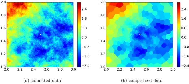
Figure 1 is an example of ASDC applied to a synthetic spatial field. Figure 1a is a simulated random field of size N = 14,400 generated from a model specified by (1) with
Y ∼ N(0, σ2
YΣ) and ∼ N(0, σ2I). The covariance matrix Σ is constructed from an
exponential model, σij = ( σ2 Y exp n −kvi−vjk θ o if kvi−vjk>0; σ2 Y +σ2 if kvi−vjk= 0, (15)
with the spatial scale parameterθ = 0.2,σ2
Y = 1, and measurement error varianceσ2 = 0.01.
Figure 1a shows simulated observations, Z(si) at each location si ∈ D. The small white
square in the center identifies a prediction region D0 consisting of a single location v0.
Figure 1bshows the corresponding compressed data for K = 400. The colors in Figure 1b are the mean data values of clusters for all locations assigned to the same cluster, as encoded by matrix Q. Very small or singleton clusters are formed around v0, and larger clusters
(a) simulated data (b) compressed data
Figure 1: Simulated raw data (a) and the corresponding compressed data forK= 400 (b).
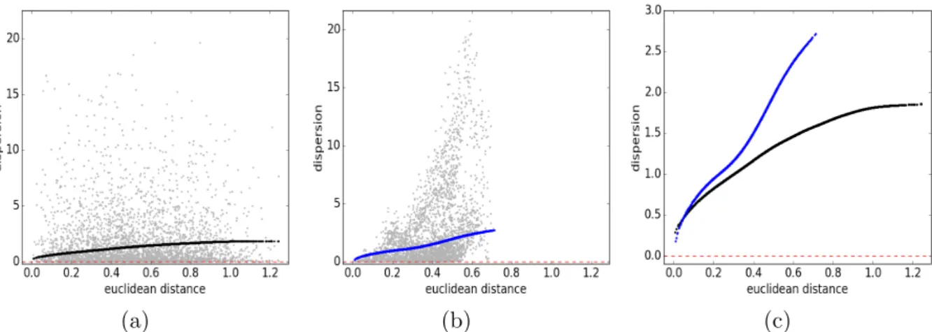
(a) (b) (c)
Figure 2: Spatial dispersions and non-parametrically fitted spatial dispersion functions. (a) spatial disper-sions{d2
e,ij}(gray) andgφˆ
e (black), (b) spatial dispersions{d 2
0,k}(gray) andgφˆ
0 (blue), (c) spline dispersion functionsgφˆe (black) andgφˆ0 (blue), where the vertical scale has been reduced.
are formed nearer to the edges of the domain. Smaller clusters preserve fine-scale spatial information around the prediction location.
Figures 2a and 2b show the spatial dispersions and the corresponding estimated spatial dispersion functions for this simulated dataset. We used cubic splines for bothgφe andgφ0 in
order to demonstrate that spatial compression can be performed even without the knowledge of the exact covariance structure of the data. Figure 2c displays the two spatial dispersion functions gφˆe and gφ0ˆ together for comparison and shows that the magnitude of the spatial
dispersions for locations in De is smaller than that between the prediction location and
locations inDe. We conclude that the spatial dependence between points in De is stronger
than is the spatial dependence between v0 and locations in De. This suggests favorable
conditions for spatial data compression. If process at v0 was independent of the process in De, then De would be compressible into a single cluster with no loss of information about
the process at v0.
2.5. Details of the ASDC algorithm
Algorithm: ASDC
Input: a block of prediction locations v0,1, . . . ,v0,M, a set of spatial locations {ve},
a set of observed spatial locations {s1, . . . ,sn} and the corresponding observed data
Z(s1), . . . ,Z(sn), number of clusters K
1: Compute two sets of spatial dispersions {d2e,ij} and {d20,`k} and the corresponding dis-tancesD(se,i,se,j) andD(s0,`,se,k):
a) d2
e,ij = (Z(se,i)−Z(se,j))2, fori, j = 1, . . . , n−m
b) d20,`k = (Z(s0,`)−Z(se,k)) 2
, for k = 1, . . . , n−m, `= 1, . . . , m 2: Fit gφe and gφ0 to {d
2
e,ij} and {d20,`k}, respectively, as per (6). That is, obtain estimates
ˆ
φe and ˆφ0, resulting in:
a) n gφˆe(D(ve,i,ve,j)) :i, j = 1, . . . , N o b) ngφ0ˆ (D(v0,`,ve,k)) :`= 1, . . . , M, k = 1, . . . , N o
3: Construct Hfrom (13) and h0,i from (14), fori= 1, . . . N
4: Construct W from (7)
5: Apply the spectral clustering algorithm toW, and obtain cluster assignments
6: Construct clusters Γj as in (2)
7: Compute cluster averagesψ(Γj) per (3) to obtain the compressed dataset:
Ψ= (ψ(Γ1), . . . , ψ(ΓK+M)) T
We demonstrate the performance of ASDC for inference and prediction in the next section. For the simulation, we make specific choices for gφe and gφ0 and use a block of
prediction locationsD0.
3. Simulation experiments
In this section we evaluate the performance of ASDC and compare it to that of two often-used alternatives: subsetting and coarse-scale aggregation. Performance of a data reduction method is characterized by simulating an ensemble of synthetic spatial fields from a known exponential covariance function, withholding the data from D0 at the center of the spatial
field to be used as a validation set, and applying kriging to the remaining data inDe, after
compression, to predict the values in D0. The exponential function with known parameters
is used to compute kriging covariance matrices as well as the parametric form of both gφe
and gφ0. The quality of these predictions over D0 is quantified by the root mean squared prediction error, RMSPE = v u u t 1 M M X i=1 (y(v0,i)−yˆ(v0,i))2, (16)
where y(v0,i) is the true value of the process (with no measurement error) at prediction
location v0,i, i = 1, ..., M, M =|D0|, and ˆy(v0,i) is the corresponding predicted value. We
run the experiment four times using 1) the uncompressed (full) data in De, 2) data in De
reduced using ASDC, 3) data in De reduced by using only a subset of locations nearest to D0, and 4) data reduced by binning the data on a coarse spatial grid and then averaging by
grid cell. For easy reference later, we refer to these four cases as full”, adaptive”, “K-local”, and “K-binned”, respectively. In cases 2), 3), and 4), we ensure that the size of the compressed datasets is the same across cases so that differences in RMSPE reflect differences in the choice of compression strategy. The quality of each of the three compression methods is measured by their RMSPE’s relative to that obtained in case 1), i.e., where there is no compression.
We perform a set of experiments to obtain distributions of RMSPE values for the three compression strategies, relative to the no-compression case, for a) several different spatial covariance structures in the underlying field, b) several different magnitudes of measurement errors in the observations, and c) two choices for the level of compression achieved. For each combination of a) and b), we generated 100 synthetic random spatial fields. Then, we compressed the data inDe six times: using each of the three compression methods for both
coarse and fine compression. Kriging was applied to De for the 100 simulations in each of
the six ensembles, and to the uncompressed data inDe, which provides a benchmark. This
yielded 100 RMSPE’s for each combination of compression method and compression level, within each combination of spatial covariance structure and measurement error. Details of these steps are given below.
The experimental design crosses the four data-reduction strategies (including the full-data case) with four spatial scale parameters for the underlying spatial model and five signal-to-noise values for the synthetic data. We summarize the results of these experiments graphically and with an analysis of variance that provides estimates of the main effects due to data reduction method, spatial scale, and signal-to-noise, and their two-way interactions. To assess robustness to the level of compression desired (parameterized by the choice ofK), the analysis is performed for both fine (K = 600) and coarse (K = 200) compression.
3.1. Generating synthetic fields
To create synthetic spatial fields, we generated stationary noisy data, according to (1), with Y ∼ N(0, σ2YΣ) for σY2 = 1 and ∼ N(0, σ2I). The covariance matrix, Σ, obtained from the isotropic exponential model in (15), where recall thatθ is the spatial scale parame-ter. We generated fields of sizeN = 100×100 = 10,000 on [0,1]×[0,1] for all combinations of four spatial scale parameters θ = {0.1,0.5,4,20} and five measurement-error variances
σ2
= {0.01,0.1,0.5,1.5,10}. Signal-to-noise ratio is defined by SNR = σY2/σ2. Thus, the
measurement-error variances correspond to SNR ={100,10,2,0.7,0.1}. For the mechanics of spatial field generation given a covariance structure, see for example Cressie(1993).
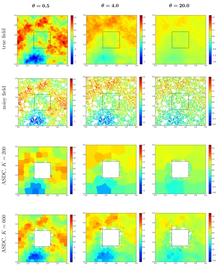
Examples of simulated complete fields for spatial scale parameters θ = {0.5,4,20} are shown in the top row of Figure 3. We omit θ = 0.1 in the figures since the result for this scale parameter were similar to those with θ = 0.5. The corresponding data with added measurement error and missing locations are shown in the second row of Figure 3. Since we anticipate that one important application of ASDC will be to remote sensing data, we chose 40% of the locations in each realization of the spatial field to be designated as missing and removed their data values. About half of the missing locations were chosen randomly and the other half were chosen around randomly generated “centers”, and hence spherical missing areas are seen in the second row of Figure3. The square outline in the center of the region shows the subdomain of interest, D0, where predictions are made. There are M =
1089 (33 × 33) locations in D0. The simulated data for these locations are set aside and used later to evaluate the quality of the kriged predictions via RMSPE.
3.2. Adaptive compression of synthetic fields
The bottom two rows of Figure 3 show the ASDC-compressed data. The second row from the bottom shows coarse compression done with K = 200 spatial clusters, and the bottom row shows fine compression with K = 600 spatial clusters. This simulation used an SNR of 10. The locations in De with missing data are assigned to spatial clusters with the
nearest geographic center, but they obviously do not contribute to the calculation of the cluster average.
Two features of the ASDC-compressed field are worth noting. First, spatial clusters near the subdomain of interest are typically smaller than those further away. This reflects the fact that spatial structure is maintained with greater fidelity at nearby locations than at locations further away, and the larger the spatial scale parameter, θ, the larger is the set of “nearby” locations. Second, clusters tend to be more or less of the same geographic size for a given radial distance away from the center of D0. This feature is a consequence of the
true field θ= 0.5 θ= 4.0 θ= 20.0 noisy field ASDC, K = 200 ASDC, K = 600
Figure 3: Top row : simulated true fields, θ = 0.5 (left), θ = 4 (center), and θ = 20 (right). Second row: corresponding noisy field with SNR = 10 and missing locations. Bottom two rows: corresponding ASDC-compressed fields forK= 200 and K = 600, where the region of interest inside the black square is
isotropic exponential function that is used to define the spatial clusters. The compressed data vectorΨ= (ψ(Γ1), . . . , ψ(ΓK))
T
replaces the original data inDe, resulting in data-size
reductions of 89% and 96%, for the K = 600 and K = 200 cases, respectively, relative to the original size of De.
Note also that for K-adaptive (i.e., ASDC), data values associated with locations in the compressed domainDecan no longer be treated as point-referenced data, since they now have
block support. This is also true for compressed data produced by K-binned. When kriging is applied to compressed fields produced by these two methods, the covariance matrices used in kriging must account for this block support. The spatial covariance matrices used to krige in the K-adaptive and K-binned cases can easily be computed using the bilinearity property of the covariance function:
¯ σk` = 1 |Ck||C`| X i0∈C k X j0∈C ` σi0j0,
whereCk and C` represent k-th and`-th clusters and σi0j0 is defined in (15).
3.3. Experimental results
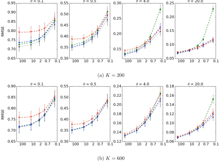
Figure 4 shows the results of our simulation experiments. Each subplot represents the average RMSPE’s, over the 100 trials of our experiments, with their 95% confidence intervals as functions of log10(SNR). Figure 4aand 4bshow the results for fine (K = 200) and coarse (K = 600) compression, respectively. The four panels in each row represent increasing spatial scale parameters in the underlying exponential model.
Although K-adaptive does not always achieve the lowest RMSPE, it is either the best, or nearly so, over the wide range of parameter choices used here. For a large SNR and across the four spatial scale parameters, K-adaptive and K-local show similar performance nearly comparable to that of K-full, and K-binned performs worse than the others, probably due to the fact that any possible strong correlations on the edges of D0 might be dampened by binning. As the spatial scale parameter increases (subplots from left to right) and the SNR decreases (along the x-axis), the performance of K-local deteriorates, especially for
K = 200, while the performance of K-binned improves. This might be because the longer correlation lengths mean that additional information from locations further away from D0
is not being used by K-local, while it is being used by K-adaptive and K-binned to improve the predictions in the high-noise scenarios.
K-adaptive has the most stable performance across all scenarios. Even though K-adaptive performs only as well as K-local in low noise, short-scale scenarios, K-adaptive outperforms
(a)K = 200
(b)K = 600
Figure 4: Plot of the mean RMSPE and its 95% confidence interval for K-adaptive (blue), K-local (green), K-binned (red), and K-full (black dotted line). Each subplot represents scale parametersθ={0.1,0.5,4,20}, respectively. On the x-axis is the logarithm of the SNR, labeled as the actual SNR ={100,10,2,0.7,0.1}. On they-axis is the mean RMSPE over 100 samples with its 95% confidence interval indicated by the error bars around the mean value.
K-local when data are noisy. Conversely, when SNR is low, K-adaptive and K-binned are comparable, but when SNR is high, K-binned’s performance deteriorates, but K-adaptive’s does not. In real-world applications, where we do not know the true values of θ or SNR, K-adaptive would be the choice with the lowest risk. Finally, K-adaptive achieves good performance and is relatively stable for both choices of K, and hence it may be especially useful in situations when high levels of data reduction are needed.
The preceding analysis focuses on the performance of the three candidate data reduction methods with respect to their predictions. It is equally important to ask how well these methods do in providing accurate estimates of prediction variance, which we measure via
θ = 0 . 5 SNR = 100 (a) SNR = 2 (b) SNR = 0.1 (c) θ = 4 (d) (e) (f) θ = 20 (g) (h) (i)
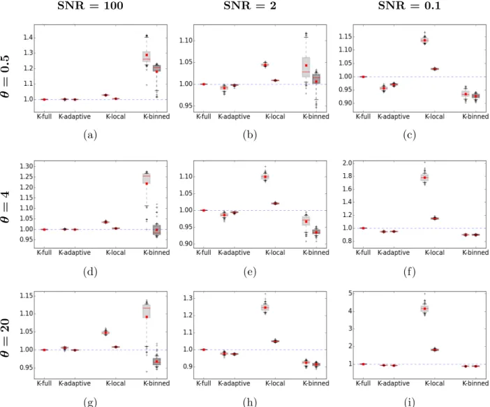
Figure 5: Boxplots of MPEVR for K-full, K-adaptive, K-binned, and K-local. Each row represents a different scale parameterθand each column represents a different SNR. The color of the boxplots is as follows: dark gray color is for K-full, light gray forK= 200, and for medium gray forK= 600. Values of the prediction error ratio closer to 1 are better.
mean prediction error variance ratio:
MPEVR = 1 M M X i=1 var(˜y(v0,i)) var(ˆy(v0,i)) , (17)
where ˜y(v0,i) represents a predicted value from K-full, and ˆy(v0,i) is a predicted value from
kriging based on a compressed dataset. The boxplots in Figure 5 show MPEVR produced when kriging is applied to compressed data under different configurations of the parameters
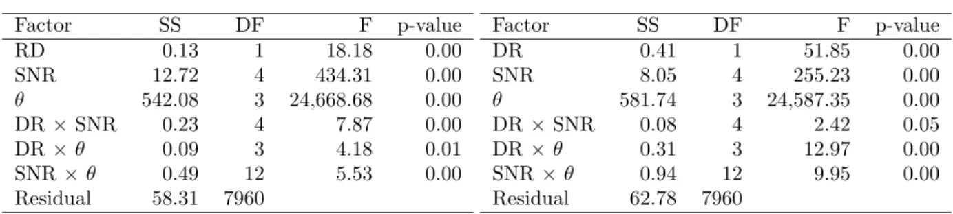
Table 1: ANOVA on RMSPE’s for all the significant factors and interactions.
(a) K-adaptive vs. K-local
Factor SS DF F p-value RD 0.13 1 18.18 0.00 SNR 12.72 4 434.31 0.00 θ 542.08 3 24,668.68 0.00 DR ×SNR 0.23 4 7.87 0.00 DR ×θ 0.09 3 4.18 0.01 SNR×θ 0.49 12 5.53 0.00 Residual 58.31 7960 (b) K-adaptive vs. K-binned Factor SS DF F p-value DR 0.41 1 51.85 0.00 SNR 8.05 4 255.23 0.00 θ 581.74 3 24,587.35 0.00 DR×SNR 0.08 4 2.42 0.05 DR×θ 0.31 3 12.97 0.00 SNR×θ 0.94 12 9.95 0.00 Residual 62.78 7960 θ, σ2
(equivalently SNR), and K. The closer the ratios are to one, the more accurate are
the prediction variances produced using compressed data.
Each of the nine panels in Figure 5corresponds to a unique combination of θ and SNR. Within each panel, the first boxplot labeled K-full is always equal to 1. For K-adaptive, K-local, and K-binned, there are two boxplots each; one corresponds to compression with
K = 200 (coarse compression), and one to K = 600 (fine compression). In all panels, the dashed horizontal line is for K-full, the benchmark. The K-adaptive MPEVR is closest to 1 in almost all cases. In panel 5c, where both SNR and θ are small, K-local does well for largerK, but K-adaptive is competitive. These conditions are closest to having a very weak spatial structure relative to the noise level and are in line with our results for RMSPE in Figure4. Once again, K-adaptive is the most robust choice over the wide range of possible conditions given in the simulation.
3.4. Analysis of variance
In this section, we quantify the results that are inferred from graphs presented in Sec-tion 3.3 through a formal analysis of variance (ANOVA). The factors are data reduction (DR) methodology, spatial scale (θ), and SNR, and the response variable is RMSPE. Since the RMSPE’s for the simulation studies were approximately symmetrically distributed, a multi-factor ANOVA is appropriate for this study. Table 1 shows the main factors and all significant two-way interactions. We further separated the analysis to compare K-adaptive to K-local in Table1aand to K-binned in Table1b. All the factors, including data-reduction method, spatial scale, and SNR have large F-statistics for both sets of comparisons. The significance of the interaction effects is slightly different for K-adaptive compared to K-local versus K-adaptive compared to K-binned. Interaction DR×SNR is stronger for K-adaptive versus K-local, confirming that noisy data have a greater impact on the performance of
K-local. On the other hand, the interaction DR×θ for K-adaptive versus K-binned indi-cates that K-binned will be impacted to a greater degree by spatial scale (i.e., length of spatial correlations). Overall, the main factors and interactions all confirm that K-adaptive provides significant improvements over the other data reduction strategies.
The principal results of the simulation experiments can be summarized as follows: – SNR is the most important factor and spatial scale is the second most important factor
determining the performance of kriging applied to compressed data.
– K-adaptive (ASDC) has the most stable and consistent performance across all scenar-ios; this is an advantage when working with real data, where the true properties of the spatial field are unknown. By comparison, K-local and K-binned exhibit oppo-site trends in performance: K-local performs worse for small SNR and large spatial scale parameters, and K-binned performs worse for large SNR and small spatial scale parameters.
– K-adaptive (ASDC) produces the most reliable prediction variances.
– K-adaptive (ASDC) performs well for very coarse levels of compression and can be effective for when drastic data reduction is needed.
3.5. Computational costs
In this section we compare the computational cost of K-full and that of ASDC. Compu-tational complexity of kriging isO(n3), where n is the number of observed locations. Since
the compressed dataset is much smaller in size than the full data, the computational cost of kriging itself based on compressed data become negligible. Therefore, we focus here on computational costs of ASDC. We do not consider the costs of fitting the spatial dispersion function as they would be the same for both full kriging (fitting the variogram) and ASDC. The costs of ASDC can be roughly separated into three components: the construction of the similarity matrix, the eigenvalue decomposition, and the K-means algorithm. The computational cost of a standard K-means algorithm (e.g., Hartigan and Wong (1979)) is considered linear in practice (Jain et al., 1999; Duda et al., 2012); for ASDC, it will depend linearly on the number of spatial locations in De, N − M, and on the number
of clusters, K, which is very small. The eigenvalue decomposition is O((N − M)3) in
computational complexity, however sparse matrix techniques can be used to bring it down to be approximately between linear and quadratic, i.e.,O((N−M)K) (Song et al.,2008), with
K n < N. Finally, the construction of the similarity matrix isO((N−M)2), but a large, 20
dense matrix H must be computed initially and will likely challenge memory limitations when N is large. Thus, the computational bottleneck for ASDC is the construction and storage of the similarity matrix. This can be addressed by constructingHas a sparse matrix (Hastie et al., 2015), and options such as rank or dimension reduction can be employed (e.g., Katzfuss, 2016). A detailed analysis of computational complexity and memory usage in spectral clustering, including sparse matrix eigen-decomposition, can be found in Song et al. (2008).
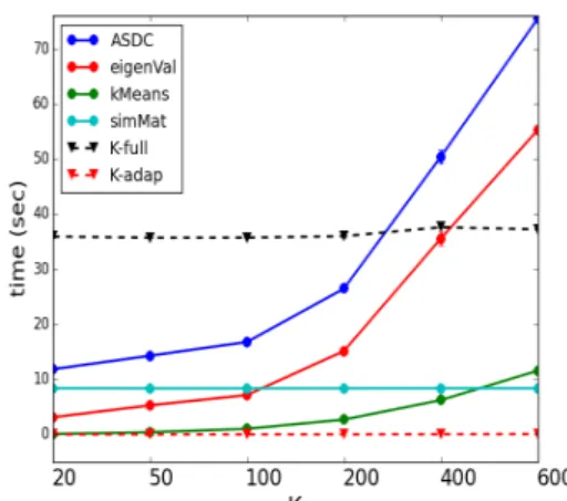
(a) Computation time (seconds) vs. size of the spatial domain.
(b) Computation time (seconds) vs. num-ber of clustersK for a square domain of size 120×120.
(c) RMSPE vs. size of spatial domain. (d) RMSPE vs. the number of clusters K
for a square domain of size 120×120.
Figure 6: Computational costs and RMSPE of K-full vs. K-adaptive (ASDC).
Figure 6 shows our analysis of computation times for K-full and K-adaptive (ASDC) in our synthetic example. Figure 6a shows computation time in seconds as a function of
increasing numbers of spatial locations, N = {602,802,1002,1202,1302,1402}, for K-full
and for K-adaptive with 99% target compression (K = 200). The overall computation time for ASDC (blue) is further separated into the construction of the similarity matrix (cyan), the eigenvalue decomposition (red), and theK-means algorithm (green). The times are averages over B = 100 randomly generated spatial fields, for each value of N, as in Section3.1. The parameters of the exponential model are fixed atθ = 0.5 and SNR = 100, with no missing data. Additional experiments (not described here) show that other choices of these parameters do not greatly affect computation time. The computational costs of kriging based on ASDC-compressed data (red dotted line) are negligible. Overall, Figure6a shows that ASDC (solid blue line) scales better than K-full (dashed black line) as the data size increases. Figure 6c shows the corresponding RMSPE averages and 95% confidence intervals for K-full and K-adaptive. K-adaptive RMSPE’s converge to those for K-full asN
increases. The sizes of the compressed datasets also increase slightly, but the compression ratio remains constant, i.e., 99%. This indicates that as the size of the data increases, ASDC could efficiently preserve the information contained in the full dataset at a proportionally decreasing computational cost.
Figure6bshows how ASDC computation time for a dataset of sizeN = 1202 varies with
decreasing compression level, i.e., as the number of clusters, K, increases. ASDC overall computation time is decomposed as in Figure 6a. The overall computation time (blue) increases approximately cubically, and is driven primarily by the eigenvalue decomposition (red). ASDC’s computation time reaches K-full’s computation time at about K = 300, which is about 98% compression. Figure6dshows that the accuracy of the prediction based on ASDC, as measured by RMSPE, reaches that of K-full at aboutK = 200 or slightly under 99% compression. This shows that ASDC can reduce computational costs of kriging on large datasets with relatively small loss of information content and predictive performance. We provide an additional discussion of computational challenges in Section5.
4. Sea-surface temperature (SST) data
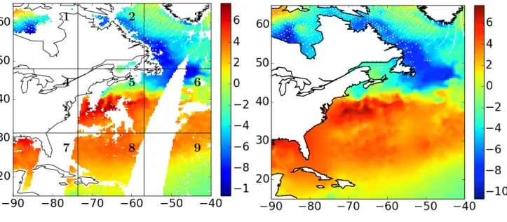
In this section we demonstrate the use of ASDC on a modest set of data from the Advanced Microwave Scanning Radiometer 2 instrument (AMSR-2; Wentz et al.(2014)) in order to show how ASDC performs when we do not know the true spatial model. These data are representative of spatial structure and patterns of missingness that are characteristic of remote sensing data. We focus on a 50◦ ×50◦ region in the north Atlantic ocean just off the east coast of the US and Canada as shown in Figure 7. We call this area the Gulf
Stream region, and it is important because of large fish populations in the area. The Gulf Stream region includes some coastlines; these areas are particularly important because this is where upwelling (the movement of cold, nutrient-rich water towards the surface) occurs. Upwelling information is an important predictor of fishery productivity and ocean-circulation (Vazquez-Cuervo et al., 2013).
We subdivide this region into into nine equal-size, non-overlapping square subregions, delineated by the black lines in Figure7a. For each subregion, we make three sets of kriging predictions, one each using ASDC-compressed data (K-adaptive), data binned to a coarse resolution (K-binned), and data in a local neighborhood (K-local). The data is compressed only in the exterior and is retained as is in the prediction region. We then compare these predictions to the full-data prediction (K-full), depicted in Figure 7b, as we did in the simulation study presented in Section3.3.
The reason for breaking the domain into nine separate subdomains is twofold. First, the spatial distributions of observations within these subdomains are different, and collectively they are representative of the kinds of patterns of missingness one often encounters in remote sensing. For example, subdomains 3 and 8 have relatively good data coverage, with missing data concentrated in relatively small contiguous areas because the missingness is caused by
1 2 3
4 5 6
7 8 9
(a) Detrended AMSR-2 SST, daytime on July 13, 2015.
(b) Predictions based on K-full.
Figure 7: Detrended SST and corresponding kriging predictions based on the full dataset. The color scale is in◦K.
areas between satellite overpasses. Subdomains 6 and 9 are missing observations over about half their domains; in subregion 6 the missing area is approximately in the center, while in subdomain 9 it is all to one side, also due to the satellite orbit. Subdomain 7 is similar to subdomain 6, but with a larger proportion of missingness; subdomain 5 has missing data due to both coastline and precipitation, through which AMSR-2 can not see. Subdomains 1 and 2 have quite a bit more missing data, and also appear to be missing data for reasons similar to that of subdomain 5. Finally, subdomain 4 is almost entirely missing, but does have a few observed data points in the ocean. To assess the impact of these different patterns, we report RMSPE and MPEVR for each region separately in Table 2below.
The second reason for breaking the domain into subdomains is to demonstrate what happens when data are processed in pieces. This may be required when data volumes are truly massive in order to exploit parallel processing. This “chunking” can produce edge effects when the nine kriged subdomains are recombined to create a single kriged data set. To quantify this effect, our RMSPE and MPEVR figures of merit are also reported for the entire domain as a whole in Table2.
In this analysis there are 11,800 AMSR-2 observations in the Gulf Stream region during the daytime on July 19, 2015. We detrended these data using a quadratic function of latitude, since this approximately captures the way SST decays moving from the Equator to the poles. AMSR-2 footprints are 25 km2 ellipses and we matched their centers to the
centers of hexagonal grid cells at 30 km2 resolution (Sahr et al. (2003); discrete global grid
resolution 8) superimposed on the domain. The benefits of using the hexagonal grid over a rectangular grid are well-known (Birch et al.,2007). The centers of these hexagonal cells are the prediction locations for kriging, and the subdomains contain between about 450 and 4,100 ocean prediction locations, each. Finally, K was set to 100 in all cases.
We estimated the parameters of an exponential covariance model from all data in the Gulf Stream region, and performed kriging on the full dataset (K-full) and on data com-pressed using ASDC (K-adaptive), subsetting (K-local), and binning (K-binned) as we did in the simulation study. The same covariance model was used in all four cases to avoid confounding data compression performance assessments with the quality of the covariance function estimate. The covariance function parameter estimates are ˆθ = 23.6 and ˆσ2
Y = 43.7
(◦K)2 and are obtained by fitting the exponential function with curve_fit of the scipy
Python library.
Table 2 shows RMSPE and MPEVR, defined in (16) and (17), respectively, with yi now
being the kriging prediction, based on the full dataset, for each of the nine subdomains. 24
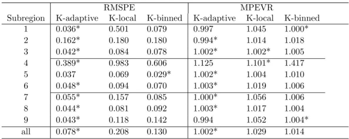
Table 2: RMSPE and mean prediction error variance ratio (MPEVR)
RMSPE MPEVR
Subregion K-adaptive K-local K-binned K-adaptive K-local K-binned
1 0.036* 0.501 0.079 0.997 1.045 1.000* 2 0.162* 0.180 0.180 0.994* 1.014 1.018 3 0.042* 0.084 0.078 1.002* 1.002* 1.005 4 0.389* 0.983 0.606 1.125 1.101* 1.417 5 0.037 0.069 0.029* 1.002* 1.004 1.010 6 0.048* 0.094 0.070 1.003* 1.019 1.006 7 0.055* 0.157 0.085 1.000* 1.056 1.006 8 0.044* 0.081 0.092 1.003* 1.017 1.004 9 0.043* 0.118 0.142 0.994 1.052 1.004* all 0.078* 0.208 0.130 1.002* 1.029 1.014
The top nine rows of Table2 summarize the performance of the three data compression methods for each of the nine prediction subregions, with starred values highlighting the best performance. The last row of the table shows performance when the kriged estimates for the nine subregions are recombined into one field. K-adaptive has the lowest RMSPE for all subdomains other than subdomain 5, where K-binned is slightly better. Recall that subdomain 5 is the only subdomain in which a significant portion of the missing data are surrounded by observed data. The MPVER for K-adaptive is best in six of the nine subdo-mains, including subdomain 5. Where K-adaptive’s performance metrics are slightly inferior to those of K-local or K-binned, it is only by a very small margin, and most likely due to the natural variation in the data. Our conclusion is that when the true pattern of missingness is not of the most favorable form, i.e., spherical, central in the domain, and not exceeding more than about half the locations, K-adaptive tends to be superior to the traditional data re-duction methods. The last row of the table combines the predictions and their uncertainties for all nine regions, and compares them to the full-kriging result. Here, K-adaptive is best in both RMSPE and MPVER, which is not surprising given the results on the individual subdomains.
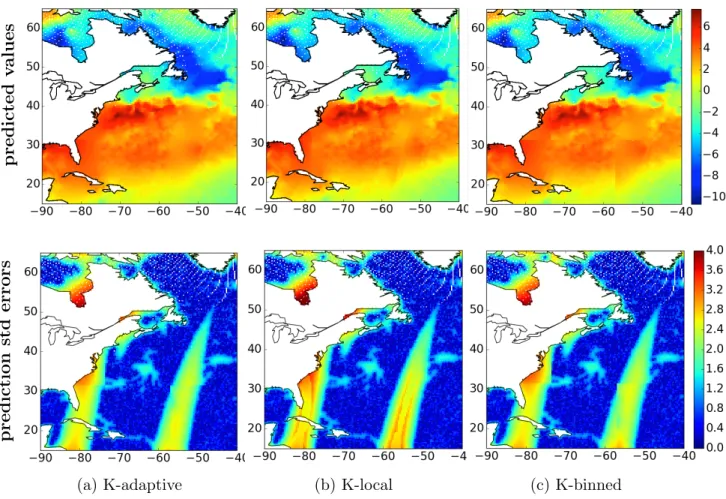
Finally, Figure 8 shows the spatial predictions and their standard errors in the Gulf Stream region for K = 100 for K-adaptive in the first column and for K-local and K-binned in the second and third columns, respectively. Differences in the predicted values across the three compression methods are small, especially at locations with corresponding observed values. Differences are evident, however, in the areas where large blocks of data are missing between satellite swaths. These differences are due to edge effects that arise when prediction is performed on several non-overlapping subregions. When K-full is used, the edge effects
predicted v alues prediction std errors
(a) K-adaptive (b) K-local (c) K-binned
Figure 8: Combined predicted SST values and their standard errors for the Gulf Stream for K-adaptive, K-local, and K-binned for a reduced dataset of size K = 100. (The regular pattern of white (missing) pixels between Labrador and Greenland are an artifact of projecting AMSR-2 data from the rectangular to hexagonal grid.
are mostly eliminated as seen in Figure 7b. Thus, in addition to its generally superior ability to preserve information, ASDC is also reduces the impact of edge effects when data are processed in chunks. The prediction standard errors obtained with K-adaptive are the closest to those of K-full as shown in Table 2. Figure 8 shows that the K-adaptive and K-binned yield lower prediction errors in the areas between swaths and in coastal regions where K-local prediction variances can be very large.
5. Summary, conclusions, and future work
In this paper, we introduced ASDC, a spatial data compression method that explicitly preserves the spatial covariance structure, and enables substantial size reductions of datasets to be used for spatial inference. We showed how ASDC uses the machinery of spectral
clustering to capture two kinds of spatial correlations. The first are those between locations outside the area in which spatial predictions are to be made, and the second are those between locations inside and outside. This strategy leads to efficient compression of the data outside while preserving information that is relevant to estimation inside the prediction area.
We studied the performance of ASDC by comparing it to two traditional methods for reducing the size of spatial data sets, subsetting and binning, in a simulation study. We generated ensembles of 100 randomly generated synthetic spatial fields from an exponential covariance model with known parameters, added measurement noise, compressed the data outside a central region of interest using ASDC and the two competitors, and then per-formed kriging to predict the data values in the region of interest. Performance is quantified through the distributions of two figures of merit over the 100-member ensemble: RMSPE, a measure of accuracy of the kriging predictions relative to the true simulated spatial field; and MPEVR, a measure of the accuracy of the kriging prediction variance, relative to that which is obtained when the original data outside are used. This experiment was conducted for various scenarios in which we used different spatial scale parameters in the exponential model used to generate the synthetic field, and different levels of measurement noise.
An important practical conclusion from this study is that ASDC is more robust to changes in spatial correlation in the underlying field, and to measurement error, than are its competitors. This robustness exists for both accuracy of prediction measured by RMSPE and, to a slightly lesser degree, to the accuracy of the prediction error measured by MPEVR. Robustness is an important advantage since we do not know the true spatial scale parameter when we work with real data. We caution, however, that this conclusion is drawn from experiments that assume an exponential covariance function. A logical next step in the simulation study is to use a different covariance model to generate synthetic spatial fields.
We used an analysis of variance to quantify the effects of the different factors in the experiment in head-to-head comparisons of the ASDC against subsetting and binning, and found that all factors (spatial scale parameter, measurement error variance, data compression method and all their interactions) are statistically significant. In fact, the most important factors are the spatial scale parameter used to generate the field and the measurement noise. To explore how computational costs scale with dataset size and degree of compression, we looked at computation times for the compound task of ASDC data compression followed by kriging. Computation time for ASDC followed by kriging is dominated by the construction of the similarity matrix and eigenvalue decomposition required by spectral clustering, but
even the total time does not go up as fast as that of kriging the full dataset. As a function of the number of spatial clusters, computation time does not rise substantially until the number of clusters reaches about 200 in our study. At the same time the RMSPE (versus truth) of the kriging predictor that uses ASDC to compress the data outside the region of interest, converges to that of kriging on the full dataset at the same number of clusters, namelyK = 200. These results suggest that a “sweet spot” exists for ASDC compression. In future work we will explore how that sweet spot depends on the structure of the underlying spatial field and on measurement error.
Finally, we applied ASDC and competitors to sea-surface temperature data from NASA’s AMSR-2 instrument by breaking these data into nine separate subregions. The subregions have different patterns of missing data, and part of the objective was to assess how these patterns might affect performance. RMSPE and MPEVR reported in Table 2 show that ASDC is also more robust to missing data than are subsetting and binning; this represents another important advantage of ASDC, since patterns of missingness in remote sensing data can depend on changing observing conditions. When the kriging predictions for the nine separate subregions were recombined, the resulting maps showed fewer edge effects when ASDC was used to pre-compress the data than were present when the alternative procedures were used. If this result is not unique to the range of experimental conditions used in this study, then it should be possible to break large datasets into non-overlapping regions and apply ASDC on those regions in parallel.
We plan additional studies to expand the range of experimental conditions used in our simulations, including other spatial covariance functions for generating synthetic fields, and modified spatial dispersion functions to incorporate geometric anisotropy (Zimmerman, 1993;Sherman,2011) in cluster formation. A number of other optimizations to our current algorithm, including exploitation of sparsity, low-rank approximations, and parallel process-ing, are on the horizon and will be necessary in order to perform ASDC on truly massive datasets in an operational data processing environment.
Acknowledgements
This work was performed at the Jet Propulsion Laboratory, California Institute of Tech-nology under contract with the National Aeronautics and Space Administration. cCopyright 2016, California Institute of Technology. All rights reserved. The authors would like to thank Drs. Michael Turmon, Jeffrey Jewell, Jorge Vazquez, Jonathan Hobbs, and Vineet Yadav for their helpful comments and discussion. Cressie’s research was partially supported by NASA
grant NNHII-ZDA001N-OCO2, and by a 2015-2017 Australian Research Council Discovery Project, DP150104576.
Ambroise, C., Dang, M., Govaert, G., 1997. Clustering of spatial data by the EM algorithm. geoENV I – Geostatistics for Environmental Applications, 493–504.
Arthur, D., Vassilvitskii, S., 2007. K-means++: The advantages of careful seeding. In: Proceedings of the Eighteenth Annual ACM-SIAM Symposium on Discrete Algorithms. Society for Industrial and Applied Mathematics, pp. 1027–1035.
Banerjee, S., Gelfand, A., Finley, A., Sang, H., 2008. Gaussian predictive process models for large spatial data sets. Journal of the Royal Statistical Society: Series B (Statistical Methodology) 70 (4), 825–848. Besag, J., Kooperberg, C., 1995. On conditional and intrinsic autoregressions. Biometrika 82, 733–746. Birch, C., Oom, S. P., Beecham, J. A., 2007. Rectangular and hexagonal grids used for observation,
experi-ment and simulation in ecology. Ecological Modelling 206 (3), 347–359.
Bornn, L., Shaddick, G., Zidek, J., 2012. Modeling non-stationary processes through dimension expansion. Journal of the American Statistical Association 107 (497), 281–289.
Chen, W., Song, Y., Bai, H., Lin, C., Chang, E., 2011. Parallel spectral clustering in distributed systems. Pattern Analysis and Machine Intelligence, IEEE Transactions on, 33 (3), 568–586.
Chung, F., 1997. Spectral graph theory (Vol. 92). American Mathematical Soc.
Craddock, R., James, G., Holtzheimer, P., Hu, X., Mayberg, H., 2012. A whole brain fMRI atlas generated via spatially constrained spectral clustering. Human Brain Mapping 33 (8), 1914–1928.
Cressie, N., 1993. Statistics for Spatial Data. New York, NY, Wiley.
Cressie, N., Johannesson, G., 2008. Fixed rank kriging for very large spatial datasets. Journal of the Royal Statistical Society: Series B (Statistical Methodology) 70 (1), 209–226.
Datta, A., Banerjee, S., Finley, A., Gelfand, A., 2015. Hierarchical nearest-neighbor Gaussian process models for large geostatistical datasets. Journal of the American Statistical Association (just-accepted) 00 (00), 00–00.
Duda, R., Hart, P., Stork, D., 2012. Pattern classification. John Wiley & Sons.
Eidsvik, J., Shaby, B., Reich, B., Wheeler, M., Niemi, J., 2014. Estimation and prediction in spatial models with block composite likelihoods. Journal of Computational and Graphical Statistics 23 (2), 295–315. Finley, A., Banerjee, S., McRoberts, R., 2009. Hierarchical spatial models for predicting tree species
assem-blages across large domains. Annals of Applied Atatistics 3 (3), 1052.
Furrer, R., Genton, M., Nychka, D., 2006. Covariance tapering for interpolation of large spatial datasets. Journal of Computational and Graphical Statistics 15 (3), 502–523.
Gramacy, R., Apley, D., 2015. Local Gaussian process approximation for large computer experiments. Jour-nal of ComputatioJour-nal and Graphical Statistics 24 (2), 561–578.
Haas, T., 1990. Kriging and automated variogram modeling within a moving window. Atmospheric Envi-ronment. Part A. General Topics 24 (7), 1759–1769.
Hammerling, D., Michalak, A., Kawa, S., 2012. Mapping of CO2 at high spatiotemporal resolution using satellite observations: Global distributions from OCO-2. Journal of Geophysical Research: Atmospheres 117 (D6).
Hartigan, J., Wong, M., 1979. Algorithm AS 136: A K-means clustering algorithm. Journal of the Royal Statistical Society, Series C (Applied Statistics) 28 (1), 100–108.
Hastie, T., Tibshirani, R., Wainwright, M., 2015. Statistical learning with sparsity: the lasso and general-izations. CRC Press.
Hu, T., Sung, S., 2006. A hybrid EM approach to spatial clustering. Computational Statistics and Data Analysis 50 (5), 1188–1205.
Jain, A., Murty, M., Flynn, P., 1999. Data clustering: a review. ACM computing surveys (CSUR) 31 (3), 264–323.
Katzfuss, M., 2016. A multi-resolution approximation for massive spatial datasets. Journal of the American Statistical Association (forthcoming).
Kaufman, C., Schervish, M., Nychka, D., 2008. Covariance tapering for likelihood-based estimation in large spatial data sets. Journal of the American Statistical Association 103 (484), 1545–1555.
Lindgren, F., Rue, H., Lindstr¨om, J., 2011. An explicit link between gaussian fields and gaussian markov random fields: the stochastic partial differential equation approach. Journal of the Royal Statistical Society: Series B (Statistical Methodology) 73 (4), 423–498.
Ng, A., Jordan, M., Weiss, Y., 2002. On spectral clustering: analysis and an algorithm. In: T. Dietterich, S. Becker, and Z. Ghahramani (Eds.) Advances in Neural Information Processing Systems. Vol. 14. MIT Press, pp. 849–856.
Nguyen, H., Cressie, N., Braverman, A., 2012. Spatial statistical data fusion for remote sensing applications. Journal of the American Statistical Association 107 (499), 1004–1018.
Nychka, D., Bandyopadhyay, S., Hammerling, D., Lindgren, F., Sain, S., 2015. A multi-resolution gaussian process model for the analysis of large spatial datasets. Journal of Computational and Graphical Statistics 24 (2), 579–599.
Papp, D., Alizadeh, F., 2014. Shape-constrained estimation using nonnegative splines. Journal of Computa-tional and Graphical Statistics 23 (1), 211–231.
Rue, H., Held, L., 2005. Gaussian Markov random fields: theory and applications. CRC Press.
Sahr, K., White, D., Kimerling, A., 2003. Geodesic discrete global grid systems. Cartography and Geographic Information Science 30 (2), 121–134.
Sampson, P., Guttorp, P., 1992. Nonparametric estimation of non-stationary spatial covariance structure. Journal of the American Statistical Association 87 (417), 108–119.
Sang, H., Huang, J., 2012. A full scale approximation of covariance functions for large spatial data sets. Journal of the Royal Statistical Society, Series B (Statistical Methodology) 74 (1), 111–132.
Sherman, M., 2011. Spatial statistics and spatio-temporal data: covariance functions and directional prop-erties. John Wiley & Sons.
Shi, J., Malik, J., 2000. Normalized cuts and image segmentation. EEE Transactions on Pattern Analysis and Machine Intelligence 22 (8), 888–905.
Song, Y., Chen, W., Bai, H., Lin, C., Chang, E., 2008. Parallel spectral clustering. In: Joint European Conference on Machine Learning and Knowledge Discovery in Databases. Springer Berlin Heidelberg, pp. 374–389.
Tobler, W., 1970. A computer movie simulating urban growth in the detroit region. Economic Geography 46 (2), 234–240.
Vazquez-Cuervo, J., Dewitte, B., Chin, T., Armstrong, E., Purca, S., Alburqueque, E., 2013. An analysis of sst gradients off the peruvian coast: The impact of going to higher resolution. Remote Sensing of
Environment 131, 76–84.
Von Luxburg, U., 2007. A tutorial on spectral clustering. Statistics and Computing 17 (4), 395–416. Wentz, F., Meissner, T., Gentemann, C., Hilburn, K., J., S., 2014. Remote Sensing Systems GHRSST Level
2P Global Subskin Sea Surface Temperature from the Advanced Microwave Scanning Radiometer 2 on the GCOM-W satellite. Ver. 7.2. Remote Sensing Systems, PO.DAAC, CA, USA.
Wever, U., 1988. Non-negative exponential splines. Computer-aided Design 20 (1), 11–16.
Zare, H., Shooshtari, P., Gupta, A., Brinkman, R., 2010. Data reduction for spectral clustering to analyze high throughput flow cytometry data. BMC Bioinformatics 11 (1), 403.
Zelnik-Manor, L., Perona, P., 2004. Self-tuning spectral clustering. In: Advances in Neural Information Processing Systems. pp. 1601–1608.