Received February 8, 2018, accepted March 14, 2018, date of publication March 26, 2018, date of current version April 23, 2018.
Digital Object Identifier 10.1109/ACCESS.2018.2817548
Robust Fault Tolerant Control for Discrete-Time
Dynamic Systems With Applications to Aero
Engineering Systems
XIAOXU LIU1, (Student Member, IEEE), ZHIWEI GAO 1, (Senior Member, IEEE),
AND AIHUA ZHANG 2
1Faculty of Engineering and Environment, Northumbria University, Newcastle upon Tyne NE1 8ST, U.K. 2College of Engineering, Bohai University, Jinzhou 121000, China
Corresponding author: Zhiwei Gao ([email protected])
This work was supported in part by NSFC under Grant 61673074, in part by the Alexander von Humboldt Foundation under Grant GRO/1117303 STP, and in part by the E&E Faculty, University of Northumbria.
ABSTRACT Unexpected faults in actuators and sensors may degrade the reliability and safety of aero engineering systems. Therefore, there is motivation to develop integrated fault tolerant control techniques with applications to aero engineering systems. In this paper, discrete-time dynamic systems, in the presence of simultaneous actuator/sensor faults, partially decoupled unknown input disturbances, and sensor noises, are investigated. A jointly state/fault estimator is formulated by integrating an unknown input observer, augmented system approach, and optimization algorithm. Unknown input disturbances can be either decou-pled by an unknown input observer, or attenuated by a linear matrix inequality optimization, enabling the estimation error to be input-to-state stable. Estimator-based signal compensation is then implemented to mitigate adverse effects from the unanticipated actuator and sensor faults. A pre-designed controller, which maintains normal system behaviors under a fault-free scenario, is allowed to work along with the presented fault tolerant mechanism of the signal compensations. The fault-tolerant closed-loop system can be ensured to mitigate the effects from the faults, guarantee the input-to-state stability, and satisfy the required robustness performance. The proposed fault estimation and fault tolerant control methods are developed for both discrete-time linear and discrete-time Lipschitz nonlinear systems. Finally, the proposed techniques are applied to a jet engine system and a flight control system for simulation validation.
INDEX TERMS Discrete-time systems, aero engineering systems, fault estimation, partically decoupled unknown inputs, signal compensation.
I. INTRODUCTION
Working under challenging operating conditions, real engi-neering systems are unavoidably subjected to abnor-mal/faulty behaviors, which degrade the functionality of the systems. Consequently, there is a high demand to develop advanced fault diagnosis and fault tolerant control strategies for enhancing the system reliability and safety. A variety of fault diagnosis and fault tolerant control techniques were developed during last decades (see [1]–[4]). Among indus-trial plants, aero systems are extremely safety-critical; hence, the level of fault diagnosis and tolerant control is required to be even higher. Therefore, fruitful results in terms of advanced fault diagnosis and tolerant control for aero engi-neering systems were documented, which can be found in the review work [5], [6].
Fault estimation/reconstruction is a multi-mission fault diagnosis technique, which can provide rich information of faults and allow successful design of fault tolerant con-troller to mitigate the influences from unexpected faults. Specifically, advanced observer methods, such as sliding mode observer [7], [8], and augmented observers [9]–[11], were applied to design state/fault estimator-based fault tol-erant controller for aerospace systems corrupted with actu-ator/sensor faults. Actuactu-ator/sensor fault reconstruction for aircraft was proposed in [12]. Fault estimations for discrete-time systems were developed in [13]–[15]. Among various fault estimation techniques, augmented system approach pos-sesses advantages in achieving simultaneous states and faults estimation, where unmeasurable system states can be esti-mated as a byproduct.
18832
2169-35362018 IEEE. Translations and content mining are permitted for academic research only.
Once the faults can be estimated, signal compensation is known as an effective fault tolerant method, which can work with a pre-designed controller, e.g., see the pioneer-ing work [9], [10]. It takes advantages to remove/mitigate the influences from the actuator/sensor faults so that the system can work well even when a fault occurs (e.g., see [9], [10], [15], [16]). The application of sig-nal compensation to aero engine systems can be found in [12] and [13]. As signal compensators achieve fault tolerance by providing compensated signals to actuators and sensors, successful implementation of signal compensa-tion depends on effective fault estimacompensa-tion. Unknown inputs including modelling errors, uncertainties, and extra perturba-tions, etc., are unavoidable in engineering plants, but may decrease the sensitivity of fault reconstruction. Unknown input observer (UIO) [17] is then motivated to be applied for decoupling the influences from the unknown inputs when carrying out fault estimation [18], [19].
As the complexity and diversity of unknown input distur-bances increase, traditional UIO techniques cannot decou-ple all unknown inputs. UIO associated with optimization scheme was hence developed for continuous-time systems subjected to partially decoupled unknown inputs in our pre-vious work [20], where unknown inputs that cannot be decoupled by UIO were attenuated by using linear matrix inequality (LMI). Therefore, a robust estimator-based signal compensation approach was designed for a continuous-time wind turbine system corrupted by faults and partially decou-pled unknown inputs in [21]. However, the aforementioned works [20], [21] were based on continuous-time systems only, which cannot be applicable to discrete-time dynamic systems. In practice, real-time implementation of monitoring and control need to use digital signals, therefore, discrete-time diagnosis and tolerant control techniques need to be explored. As a result, it is well motivated to design robust UIO-based fault tolerant control techniques for discrete-time dynamic systems subjected to faults and partially decoupled unknown inputs, which can be applied to aero engineering systems. Due to the nature of discrete-time dynamics, some well-known techniques for continuous systems such as high-gain observer techniques etc., [9], [10], have been found difficult to apply for discrete-time systems.
In this paper, an integrated robust fault estimator-based fault tolerant control approach is addressed for discrete-time systems in presence of simultaneous faults and par-tially decoupled unknown inputs. Specifically, robust fault estimation can be obtained by integrating augmented system approach, UIO, and LMI techniques, such that the estima-tion error dynamic is input-to-state stable. Signal compensa-tion method is then developed to achieve tolerance against actuator and sensor faults, and maintain the stability of the closed-loop system. The robust fault estimator-based fault tolerant control approaches are presented for both linear and Lipschitz nonlinear discrete-time systems. The novelties and contributions of this work include: 1) Simultaneous discrete-time state/fault estimation techniques with robustness against
partially decoupled unknown inputs are developed, with the aid of input-to-stability theory. The input disturbances are assumed not to be completely decoupled, which can meet more general practical engineering conditions. 2) Robust fault estimation-based signal compensation for fault tolerant control is addressed without replacing the pre-existing con-troller, which makes the tolerant control strategies simple to apply and capable of avoiding performance fluctuations due to controllers switching. 3) Input-to-state stability theory is used for the stability proof of the estimation error dynamics and tolerant closed-loop control system, which is shown to be an effective tool for handling discrete-time estimation and control issues. 4) Case studies on two aero engineering systems are used to demonstrate the effectiveness.
The rest of the paper is organized as follows. In Section II, the UIO-based fault estimation approach is addressed for discrete-time linear dynamic systems subjected to both faults and partially decoupled unknown input uncertainties. Estimator-based signal compensation tolerant technique is developed in Section III. UIO-based fault estimation and fault tolerant control approaches for discrete-time Lipschitz nonlinear systems are presented in Section VI. The devel-oped integrated fault tolerant control strategies are demon-strated using two aero systems for case studies in Section V. The paper ends with the conclusion in Section VI.
Notation: The notations in this paper are standard.
The superscript ‘‘T’’ represents the transpose of matri-ces or vectors. Rn and Rn×m stand for the n-dimentional Euclidean space and the set ofn×mreal matrices, respec-tively. R+ and J+ represent the set of nonnegative reals
and nonnegative integers, respectively.X < 0 indicates the symmetric matrixX is negative definite, while the notation
X > Y means that X −Y is positive definite. In denotes
the identity matrix with the dimension of n × n, while 0 is a scalar zero or a zero matrix with appropriate zero entries. For a complex number z,|z| denotes the module ofz; while for a vector x,|x|refers to the Euclidean norm of the vector. |x|2 = P∞
k=0xT(k)x(k) 1/2
, and |A| =
q
λmax ATAfor a real matrixA.∀means for all. Denotes
kvk = sup{|v(k)| :k∈J+} ≤ ∞, which indicates kvk is the standard l∞ norm when v is bounded. For brevity, M1M2 ∗ M3 1 ⇐⇒ M1 M2 M2T M3 .
II. UIO-BASED FAULT ESTIMATION FOR DISCRETE-TIME LINEAR DYNAMIC SYSTEMS
Consider a discrete-time plant subjected to actuator faults, sensor faults, and unknown disturbances in the form of
(
x(k+1)=Ax(k)+Bu(k)+Bff(k)+Bdd(k)
y(k)=Cx(k)+Dff(k)+Ddds(k)
(1)
wherex(k) ∈ Rn represents state vector with initial value of x0 ∈ Rn; u(k) ∈ Rm andy(k) ∈ Rp stand for control
input vector and measurement output vector, respectively;
either disturbances or modelling errors;ds(k) ∈ Rls is the
measurement noise;f(k) ∈ Rlf is the fault vector involving
actuator faults and sensor faults; k ∈ J+ is the discrete-time instant.A,B,C,Bd,Bf,Dd andDf are known constant
coefficient matrices with appropriate dimensions. In addition,
Bd = [Bd1Bd2], d(k)=[dT1(k) d2T(k)]T, d1(k) ∈ Rld1
andd2(k) ∈ Rld2, whered1(k) rather thand2(k) is assumed
to be decoupled, andBd1is of full column rank.
Define
1f (k)=f(k+1)−f (k) (2)
and assume1f (k)is bounded. Denote ¯ n=n+lf ¯ x(k)=xT(k) fT(k)T ∈Rn¯, ¯ d(k)=dT(k) 1fT(k)T ∈Rld+lf,
Therefore, system (1) can be represented by an augmented system as follows: ( ¯ x(k+1)= ¯Ax¯(k)+ ¯Bu(k)+ ¯Bdd¯(k) y(k)= ¯Cx¯(k)+Ddds(k) (3) and the corresponding system coefficients are:
¯ A= A Bf 0lf×n Ilf ∈Rn¯× ¯n, B¯ = B 0lf×m ∈Rn¯×m, ¯ Bd = Bd 0n×lf 0lf×ld Ilf ∈Rn¯×(ld+lf), ¯ C =C Df ∈Rp× ¯n. Denote d¯2(k) = d2T(k) 1fT(k) T ∈ Rld2+lf,
andd¯(k)=[dT1(k) d¯2T(k)]T, whered1(k) can be decoupled
whereasd¯2(k) cannot be decoupled. Moreover, we letB¯d =
¯ Bd1B¯d2, where B¯d1 = Bd1 0lf×ld1 ∈ Rn¯×ld1 andB¯ d2 = Bd2 0n×lf 0lf×ld2 Ilf ∈Rn¯×(ld2+lf).
It is clear thatx¯(k) contains the original state vectorx(k) and the concerned fault vector f(k). As a result, these two components can be estimated simultaneously by designing an observer for the augmented system (3).
To attenuate the influences from the unknown inputs, a UIO can be constructed for system (3) as follows:
(
¯
z(k+1)=R¯z(k)+TBu¯ (k)+(L1+L2)y(k)
ˆ¯
x(k)= ¯z(k)+Hy(k) (4)
where¯z(k) ∈ Rn¯ is the state vector of dynamic system (4) andxˆ¯(k)∈Rn¯ represents the estimation ofx¯(k)∈Rn¯, while
R∈Rn¯× ¯n,L1∈Rn¯×p,L2∈Rn¯×p,T ∈Rn¯× ¯nandH ∈Rn¯×p
are the gain matrices to be designed. Defining the estimation error as
e(k)= ¯x(k)− ˆ¯x(k) (5)
it can be calculated that
e(k+1)= ¯x(k+1)− ˆ¯x(k+1) = In¯−HC¯¯ x(k+1)− ¯z(k+1) −HDdds(k+1) (6) Using (3)-(6), we have e(k+1) = In¯−HC¯ ¯ A−L1C¯ ¯ x(k)−Rxˆ¯(k) + In¯−HC¯ −TBu¯ (k)+ In¯−HC¯ ¯ Bd1d1(k) + In¯−HC¯B¯d2d¯2(k)−L1Ddds(k) +(RH−L2)y(k)−HDdds(k+1) (7)
Estimation error dynamic (7) can be reduced to
e(k+1)=Re(k)+TB¯d2d¯2(k)−L1Ddds(k)
−HDdds(k+1) (8)
if the following conditions hold
In¯−HC¯B¯d1=0 (9)
R= ¯A−HC¯A¯−L1C¯ (10)
T =In¯−HC¯ (11)
L2=RH (12)
In order to make conditions (9)-(12) hold, we have the following Lemma:
Lemma 1:The sufficient and necessary conditions for the existence of the UIO (4) for the system (3) are:
(i) rank(CBd1)=rank(Bd1);
(ii). rank A−In Bf Bd1 C Df 0 =n+ld1+lf; (iii). rank A−zInBd1 C 0 = n + ld1, ∀z, with |z| ≥ 1 andz6=1.
Proof:See Appendix. A special solution of (9) is H = ¯Bd1[ C¯B¯d1 T ¯ CB¯d1] −1 ¯ CB¯d1 T (13) From (8), one can seed1(k) has been decoupled, by
deriv-ingHfrom (13) to satisfy condition (9), butd¯2(k) still exists.
Therefore, the observer design is transformed to seek the observer gains to ensure the estimation errore(k)stable and attenuate the influences ofd¯
2(k) on estimation errore(k).
The following definitions and lemmas about input-to-state stability are introduced.
Definition 1 [22]:A functionγ :R+−→R+is said to be aK-function if it is continuous, strictly increasing, and satisfy
γ (0)=0.γis aK∞function if it is aK-function, and also
γ (s)→ ∞ass→ ∞.
Definition 2 [22]:A functionβ : R+×R+ −→ R+is
said to be aKL-function if for each fixedt ≥0, the function
β(s,t) is aK-function, and for each fixeds≥0, the function is decreasing, andβ(s,t)−→0 ast −→ ∞.
Consider the following discrete-time dynamic system
x(k+1)=h(x(k),v(k)) (14) wherex(k)∈ Rnis system state andv(k)∈Rvis input. For system (14), we have the following definition.
Definition 3 [23]:System (14) is said to be input-to-state stable, if there exist functionsβ ∈KLandγ ∈K, such that for any initial conditionx(k0)=x0,v(k)∈l∞v , andk ∈J+
one has
|x(k,x0,v)| ≤β (|x0|,k)+γ (kvk) (15) From Definition 3, we can know input-to-state stability takes the influences of inputs on stability into consideration, and reflects that bounded inputs result in bounded system states. It can indicate the robustness of a system.
Lemma 2 [23]–[25]:LetV : Rn → R+be a continuous
function. If there existK∞functionsψ1andψ2, such that
ψ1(|x|)≤V(x)≤ψ2(|x|), ∀x∈Rn (16)
and if there exist aK∞functionψ3and aKfunctionψ4, such
that
V(h(x,v))−V(x)≤ −ψ3(|x|)+ψ4(|v|)
∀x∈Rn, ∀v∈Rv (17) then system (14) is input-to-state stable.
Based on the definitions and lemmas above, it is time to design robust observer (4) so that the error dynamic (8) is input-to-state stable.
Theorem 1:For system (3), there exists a robust UIO in the form of (4) such that the error dynamic system (8) is input-to-state stable, if there exist a positive definite matrixPand matrixY, and the positive scalarsα,γd2,γdsandγds1 such
that inequality (18) holds, which is shown at the bottom of this page.
Furthermore, one can calculateL1=P−1Y.
Proof:Take the following Lyapunov function candidate for error dynamic system (8):
V(e(k))=eT(k)Pe(k) (19)
It is clear that
λmin(P)|e(k)|2≤V(e(k))≤λmax(P)|e(k)|2 (20)
indicating thatV(e(k))satisfies condition (16) inLemma 2, with ψ1(|e(k)|) = λmin(P)|e(k)|2, and ψ2(|e(k)|) =
λmax(P)|e(k)|2.
Defineη (k)=e(k+1)−e(k). From (8), one can derive
η (k)=(R−In¯)e(k)+TB¯d2d¯2(k)−L1Ddds(k)
−HDdds(k+1) (21)
By using (19) and (21), one can have
1V(e(k)) =V(e(k+1))−V(e(k)) =eT (k+1)Pe(k+1)−eT(k)Pe(k) =[e(k+1)−e(k)]TP[e(k+1)−e(k)] +2eT(k)Pe(k+1)−2eT(k)Pe(k) =[e(k+1)−e(k)]TP[e(k+1)−e(k)] +2eT(k)P[e(k+1)−e(k)] = −[e(k+1)−e(k)]TP[e(k+1)−e(k)] +2eT(k)P[e(k+1)−e(k)] +2 [e(k+1)−e(k)]TP[e(k+1)−e(k)] = −ηT (k)Pη (k)+2eT(k)Pη (k)+2ηT(k)Pη (k) = −ηT (k)Pη (k)+2eT(k)P(R−In¯)e(k) +2eT(k)PTB¯d2d¯2(k)−2eT(k)PL1Ddds(k) −2eT(k)PHDdds(k+1) +2ηT (k)P(R−I¯n)e(k)+2ηT(k)PTB¯d2d¯2(k) −2ηT (k)PL1Ddds(k)−2ηT(k)PHDdds(k+1) (22) Adding and subtracting
−γ2
d2d¯2T(k)d¯2(k)−γds2dsT (k)ds(k)
−γds21dsT(k+1)ds(k+1)+αV(e(k))
to the right side of (22), one has
1V(e(k)) =ηT(k) eT(k) d¯T 2(k) d T s (k) dsT(k+1) ×2 η (k) e(k) ¯ d2(k) ds(k) ds(k+1) +γd22d¯2T(k)d¯2(k)+γds2dsT (k)ds(k) +γ2 ds1dsT(k+1)ds(k+1)−αV(e(k)) (23)
where2is shown in the first equation at the top of the next page.
From (10), it is clear thatPR =PTA¯ −YC¯, whereY =
PL1. Therefore,2can be rewritten as follows, which is shown
in the second equation at the top of the next page. LMI (18) indicates2 <0, leading to
1V(e(k)) <−αV(e(k))+γ2 d2d¯2T(k)d¯2(k) +γ2 dsd T s (k)ds(k)+γds21d T s (k+1)ds(k+1) (24) −P PTA¯ −YC¯ −P PTB¯d2 −YDd −PHDd ∗ 2PTA¯−2YC¯ +(α−2)P PTB¯d2 −YDd −PHDd ∗ ∗ −γ2 d2I(ld2+lf) 0 0 ∗ ∗ ∗ −γ2 dsIlds 0 ∗ ∗ ∗ ∗ −γ2 ds1Ilds <0 (18)
2= −P P(R−In¯) PTB¯d2 −PL1Dd −PHDd ∗ 2P(R−In¯)+αP PTB¯d2 −PL1Dd −PHDd ∗ ∗ −γ2 d2I(ld2+lf) 0 0 ∗ ∗ ∗ −γ2 dsIlds 0 ∗ ∗ ∗ ∗ −γ2 ds1Ilds 2= −P PTA¯−YC¯ −P PTB¯d2 −YDd −PHDd ∗ 2PTA¯−2YC¯ +(α−2)P PTB¯d2 −YDd −PHDd ∗ ∗ −γ2 d2I(ld2+lf) 0 0 ∗ ∗ ∗ −γ2 dsIlds 0 ∗ ∗ ∗ ∗ −γ2 ds1Ilds
Since−αV(e(k)) ≤ −αλmin(P)|e(k)|2, and form (24) one can have
1V(e(k)) <−αλmin(P)|e(k)|2+γ2 d2d¯ T 2 (k)d¯2(k) +γds2dsT(k)ds(k)+γds21dsT(k+1)ds(k+1) (25) which means condition (17) in Lemma 2 is met. Specifi-cally, ψ3(|e(k)|) = αλmin(P)|e(k)|2 and ψ4(|v(k)|) = max{γ2 d2, γ 2 ds, γ 2 ds1} |v(k)| 2, in whichv(k)=¯ d2T(k) dsT(k) dsT(k+1)T
. As a result, the error dynamic system (8) is input-to-state stable. This completes the proof.
Now the design procedure of the fault estimator can be summarized as follows:
Procedure 1 (UIO-Based State/Fault Estimation):
(1) Construct the augmented system in the form of (3) for the discrete-time model (1).
(2) SolveHfrom Equation (13).
(3) Solve the LMI (18) to obtain the matricesPandY, and calculate the gainL1=P−1Y.
(4) Calculate the gain matricesR,T andL2following the
formulae (10)-(12), respectively.
(5) Generate the augmented estimatexˆ¯(k) by implement-ing UIO (4), leadimplement-ing to the simultaneous estimates of the state and fault asxˆ(k)=In 0n×lf
ˆ¯ x(k) andfˆ(k)= 0lf×nIlf ˆ¯ x(k), respectively.
III. FAULT TOLERANT CONTROL FOR DISCRETE-TIME LINEAR SYSTEM
Assume there is a pre-existing dynamic output feedback con-troller, designed for normal operating conditions (i. e., fault free scenario), in the form of
(
xc(k+1)=Acxc(k)+Bcy(k)
u(k)=Ccxc(k)
(26)
wherexc(k) ∈ Rnc is the state of the dynamic controller,
Ac,BcandCcare control gains with appropriate dimensions,
whose designs are beyond this study.
Based on the estimation ofxˆ¯, the original system state and fault vector can be reconstructed as
ˆ x(k)=In 0n×lf ˆ¯ x(k) (27) and ˆ f(k)=0lf×n Ilf ˆ¯ x(k) (28) Suppose rank B Bf =rankB (29)
and the compensated signal for the actuator is designed as
uf =Kffˆ, where
Kf =B+Bf (30)
Therefore, we have
Bf −BKf =0 (31)
Using−Dffˆ(k) to compensate the measurement output, we have yc(k)=y(k)−DfJ2xˆ¯(k) =Cx(k)+Dff(k)−Dffˆ(k)+Ddds(k) =Cx(k)+DfJ2e(k)+Ddds(k) (32) whereJ2=0lf×nIlf .
Subtracting uf from the actuator input, and using the
compensated measurement output yc to replace the actual
measurementy, the controller with signal compensation can thus be updated as follows:
(
xc(k+1)=Acxc(k)+Bcyc(k)
u(k)=Ccxc(k)−KfJ2xˆ¯(k)
Substituting controller (33) to system (1), the resulting closed-loop system can be established
( ˜ x(k+1)= ˜Ax˜(k)+ ˜Bdd˜(k)+Bee(k) yc(k)= ˜Cx˜(k)+DfJ2e(k)+Jdd˜(k) (34) where ˜ x(k)= xT(k) xcT(k)T , ˜ A= A BCc BcC Ac , ˜ Bd = Bd 0 0 BcDd , C˜ =[C 0 p×nc], ˜ d(k)=dT(k) dsT(k)T, Be= BfJ2 BcDfJ2 , andJd =[ 0p×ld Dd].
One can presume that under controller (26), the closed-loop system is input-to-state stable in fault-free scenario, with the following robustness performance
|y|2 2≤γp ˜ d 2 2 (35)
whereγpis a positive scalar.
Since system (1) is input-to-state stable under con-troller (26) for fault-free case, there is a Lyapunov functionVc
which satisfies condition (16) and (17) ofLemma 2. Without loss of generality, one can presume the Lyapunov function can be found asVc(x˜(k))= ˜xT(k)P˜x˜(k), such that
ψc1(| ˜x(k)|)≤Vc(x˜(k))≤ψc2(| ˜x(k)|) (36) and 1Vc(x˜(k)) <−αc| ˜x(k)|2+γc ˜ d(k) 2 (37) whereP˜is a positive-definite matrix with appropriate dimen-sion,ψc1,ψc2∈K∞,αcandγcare positive scalars.
Now it is ready to discuss the stability and robustness of the dynamic system (34) in faulty case after signal compensation.
Theorem 2:If there is a pre-existing controller in the form of (26) to ensure the closed-loop system of the plant (1) to be input-to-state stable under fault-free case and satisfy the robust performance index (35), the tolerant controller (32 )-(33) can drive the trajectories of the closed-loop system of the plant (1) to be input-to-state stable when a fault occurs, and satisfy the following robust performance index:
|yc|22≤γ0 ˜ d 2 2 +γ0e|e|2 2 (38)
whereγ0andγ0eare positive scalars representing the robust
performance indices.
Proof:Choose Lyapunov function as ˜
V(x˜e(k)) =Vc(x˜(k))+ξV(e(k))
= ˜xT(k)P˜x˜(k)+ξeT(k)Pe(k) (39) whereξ is a positive scalar,x˜e(k)=x˜T (k)eT(k)T.
Therefore,V˜(x˜e(k))satisfies condition (16) inLemma 1
with ψ1˜ (| ˜xe(k)|) = min{λmin(P˜), ξλmin(P)} | ˜xe(k)|2, and
˜
ψ2(| ˜xe(k)|)=max{λmax(P˜), ξλmax(P)} | ˜xe(k)|2.
From (25), one can have
1V(e(k)) <−αe|e(k)|2+γe|v(k)|2 (40) whereαe=αλmin(P) ,andγe=max{γd22, γds2, γds21}.
It should be noticed that, condition (37) holds when sys-tem (1) is free of faults. Nevertheless, considering faulty cases, the closed-loop system of (1) is subjected to the esti-mation error as shown in (34). As a result,1Vc(x˜(k))in (37)
is also corrupted with estimation errore(k)under faulty case. According to (34), (37), (39) and (40), we have
1V˜ <−α c| ˜x(k)|2+γc ˜ d(k) 2 +eT(k)BTePB˜ ee(k) +2x˜T(k)A˜TPB˜ ee(k)+2eT(k)BTeP˜B˜dd˜(k) −ξαe|e(k)|2+ξγe|v(k)|2 ≤ −αc| ˜x(k)|2+γc ˜ d(k) 2 +ξe|e(k)|2 +ξx| ˜x(k)| |e(k)| +2ξd|e(k)| ˜ d(k) −ξαe|e(k)|2+ξγe|v(k)|2 ≤ −αc| ˜x(k)|2−(−ξe+ξαe−ξd)|e(k)|2 +ξx| ˜x(k)| |e(k)| +(γc+ξd) ˜ d(k) 2 +ξγe|v(k)|2 (41)
where ξe, ξx, and ξd are positive scalars such that ξe =
B T ePB˜ e ,ξx =2 ˜ ATPB˜ e ,ξd= B T eP˜B˜d . Selecting ξ ≥ ξ 2 x+(ξd+ξe)αc αcαe (42) and from (41) and (42), one has
1V˜ ≤ −αc 2 | ˜x(k)| 2−−ξe+ξαe−ξd 2 |e(k)| 2 +ξγe|v(k)|2+(γc+ξd) ˜ d(k) 2 ≤ −αxe| ˜xe(k)|2+βxe|˜v(k)|2 (43) in which αxe = min{α2c, −ξe+ξαe−ξd 2 }, ˜v(k) = vT(k)d˜T(k)T, andβxe=max{ξγe, γc+ξd}.
Therefore, the input-to-state stability of the close-loop sys-tem (34) has been proved.
Now it is time to discuss the robustness performance of the closed-loop system (34).
Considering (34) for fault-free case and using (35), one has
XN k=0y T (k)y(k) =XN k=0[x˜ T(k)C˜TC˜x˜(k)+ ˜dT(k)JT dJdd˜(k) +2x˜T(k)C˜TJdd˜(k)] ≤ γpXN k=0 ˜ dT(k)d˜(k) (44)
For system (34) under faulty scenario, and using (44), one can derive XN k=0y T c (k)yc(k) =XN k=0[x˜ T(k)C˜TC˜x˜(k)+ ˜d(k)T JT dJdd˜(k) +2x˜T(k)C˜TJdd˜(k)+eT(k)J2TDfTDfJ2e(k) +2x˜T(k)C˜TDfJ2e(k)+2eT(k)J2TD T f Jdd˜(k)] ≤ XN k=0[(γp + J T 2DTf Jd ) ˜ d(k) 2 +( J T 2DTfDfJ2 + ˜ CTDfJ2 + J T 2DTf Jd )|e(k)| 2+ ˜ CTDfJ2 | ˜x(k)| 2] (45) Adding and subtracting PN
k=0ξ1Vc(x˜(k)) to (45), and
using (37), one can have
XN k=0y T c (k)yc(k) ≤ XN k=0[(γp+ J T 2DTf Jd +ξγc) ˜ d(k) 2 +( J T 2D T f DfJ2 + ˜ CTDfJ2 + J T 2D T fJd )|e(k)| 2 +( ˜ CTDfJ2 −ξαc)| ˜x(k)| 2−ξ1V c(x˜(k))] ≤ XN k=0[γ0 ˜ d(k) 2 +γ0e|e(k)|2 +( ˜ CTDfJ2 −ξαc)| ˜x(k)| 2]−XN k=0ξ1Vc(x˜(k)) (46) whereγ0=γp+ J T 2DTfJd +ξγcandγ0e= J T 2DTf DfJ2 + ˜ CTDfJ2 + J T 2D T fJd . Selecting ξ ≥max ξ2 x+(ξd+ξe)αc αcαe , ˜ CTDfJ2 αc (47) using (46), we have XN k=0y T c (k)yc(k)≤ XN k=0[γ0 ˜ d(k) 2 +γ0e|e(k)|2] −XN k=0ξ1Vc(x˜(k)) (48)
Under zero initial conditions, one has
XN
k=0ξ1Vc(x˜(k))=ξVc(x˜(N))≥0 (49)
As a result, the inequality (48) can be further reduced to
XN k=0y T c (k)yc(k)≤ XN k=0[γ0 ˜ d(k) 2 +γ0e|e(k)|2] (50) which indicates the robustness performance (38) holds for the closed-loop system (34). This completes the proof.
Now, we can conclude the design procedure of the robust fault estimator-based fault tolerant control strategies.
Procedure 2 (Tolerant Control With Signal Compensation):
(1) The estimate of the augmented state vectorxˆ¯ is pro-duced from the robust estimation algorithm described inProcedure 1.
(2) Based on a pre-existing controller (26), implement the tolerant controller in the form (32)-(33) with signal compensation for system (1).
Remark 1:If the pre-existing controller is a static output feedback controller in the form of
u(k)=Ky(k) (51)
so that the resulting closed-loop system of (1) under fault-free condition is input-to-state stable and satisfies the robust performance index in the form of (35), the tolerant controller becomes
u(k)=Kyc(k)−KfJ2xˆ¯(k) (52)
whereyc(k) is defined as in (32) and Kf is given by (30).
Under faulty scenario, the closed-loop system becomes:
(
x(k+1)=Akx(k)+Bkdd˜(k)+Bkee(k)
yc(k)=Cx(k)+DfJ2e(k)+Jdd˜(k)
(53) whereAk =A+BKC,Bkd =Bd BKDd,Bke=BKDfJ2+ BfJ2, and the other symbols are defined as before. Define the
storage function as
Vg(xe(k))=Vc(x(k))+ξV(e(k))
=xT(k)Qx(k)+ξeT(k)Pe(k) (54) whereP andQ are both positive definite matrices, ξ is a positive scalar, xe(k) = xT(k)eT (k)T. By using the
same proof manner of Theorem 2, one can derive the result straightforward: the tolerant controller (52) can drive the trajectories of the closed-loop system of the plant (1) to be input-to-state stable when a fault occurs, and satisfy a robust performance index in the form of (38).
IV. ESTIMATOR-BASED FAULT TOLERANT CONTROL FOR DISCRETE-TIME LIPSCHITZ NONLINEAR SYSTEMS In Sections II and III, robust simultaneous state and fault estimator and estimator-based tolerant controller are devel-oped for discrete-time linear systems. It is noted that some aero engineering systems are Lipschitz nonlinear systems, therefore, it is of interest to extend the results obtained in the Sections II and III to Lipchitz nonlinear dynamic systems. A. STATE AND FAULT SIMULTANOUES UIO-BASED ESTIMATOR FOR LIPSCHITZ NONLINEAR DISCRETE-TIME DYNAMIC SYSTEMS
A discrete-time plant with Lipschitz nonlinear constraints is described as follows: x(k+1)=Ax(k)+Bu(k)+Bff (k) +Bdd(k)+8(x(k) ,u(k)) y(k)=Cx(k)+Dff (k)+Ddds(k) (55)
where8(x(k) ,u(k)) is a Lipschitz nonlinear function vec-tor, i.e.,∀x(k),xˆ(k)∈Rn, andu(k)∈Rm, there is a constant
θ >0, such that 8 (x(k) ,u(k))−8 xˆ(k) , u(k) ≤θ x(k)− ˆx(k) (56) and the other symbols are the same as defined in (1).
Defining an augmented state vector to be x¯(k) =
xT(k)fT(k)T ∈ Rn¯, one can obtain an equivalent aug-mented system as follows:
( ¯ x(k+1)= ¯Ax¯(k)+ ¯Bu(k)+ ¯Bdd¯(k)+ ¯8(x(k),u(k)) y(k)= ¯Cx¯(k)+Ddds(k) (57) where8 (¯ x(k) ,u(k)) = 8T(x(k) ,u(k)) 01×lf T ∈ Rn¯,
and the other symbols are defined the same as those in (3). The nonlinear UIO is then designed for the augmented system (57) as follows: ¯ z(k+1)=R¯z(k)+TBu¯ (k)+T8¯ xˆ(k) ,u(k) +(L1+L2)y(k) ˆ¯ x(k)= ¯z(k)+Hy(k) (58)
whereR,T,L1,L2andHare the observer gains to be designed
by satisfying (9)-(12).
The estimation error is the same as defined as (5). From (5), (57) and (58), one can obtain the estimation error equation as
e(k+1)=Re(k)+TB¯d2d¯2(k)+T8˜(k)
−L1Ddds(k)−HDdds(k+1) (59)
where 8˜(k) = 8 (¯ x(k) ,u(k)) − ¯8 xˆ(k) ,u(k), H is obtained by (13),T is calculated by (11);R = ¯A−HC¯A¯−
L1C¯ = TA¯ −L1C¯, in whichL1 is to be designed in the
following theorem.
Theorem 3: For system (57), there exists a robust UIO
in the form of (58) such that the error dynamic system (59) is input-to-state stable, if there exist a positive definite matrixP
and matrixY, and the positive scalarsα, γd2,γds,γds1andγθ,
such that inequality (60) holds, which is shown at the bottom of this page.
Furthermore, one can calculateL1=P−1Y.
Proof: Choosing the Lyapunov function in the form
of (19), which satisfies (16) inLemma 2according to (20). Defineη (k)=e(k+1)−e(k). From (59), we can have
η (k)=(R−In¯)e(k)+TB¯d2d¯2(k)−L1Ddds(k)
−HDdds(k+1)+T8˜(k) (61)
According to (19) and (61) and using the similar manner to derive (22), we have 1V(e(k)) = −ηT(k)Pη (k)+2eT(k)Pη (k)+2ηT(k)Pη (k) = −ηT(k)Pη (k)+[2eT(k)P(R−In¯)e(k) +2eT (k)PTB¯d2d¯2(k)+2eT(k)PT8 (˜ k) −2eT (k)PL1Ddds(k)−2eT(k)PHDdds(k+1) +2ηT(k)P(R−In¯)e(k)+2ηT (k)PTB¯d2d¯2(k) +2ηT(k)PT8 (˜ k)−2ηT(k)PL1Ddds(k) −2ηT(k)PHDdds(k+1) (62)
Adding and subtracting
−γθ8˜T(k)8 (˜ k)−γd22d¯2T(k)d¯2(k)−γds2dsT(k)ds(k)
−γ2
ds1dsT(k+1)ds(k+1)+αV(e(k))
to the right side of (62), one has
1V(e(k)) ≤ ηT(k) eT(k) d¯2T(k) dsT(k) dsT(k+1) 8˜T(k) × η (k) e(k) ¯ d2(k) ds(k) ds(k+1) ˜ 8 (k) +γd22d¯2T(k)d¯2(k)+γds2dsT(k)ds(k) +γ2 ds1dsT(k+1)ds(k+1)−αV(e(k)) (63)
whereis shown at the top of the next page. From the LMI (60), it is evident that
<0 (64) indicating 1V(e(k)) < −αV(e(k))+γ2 d2d¯ T 2 (k)d¯2(k) +γds2dsT(k)ds(k)+γds21dsT(k+1)ds(k+1) ≤ −αλmin(P)|e(k)|2+γd22d¯2T(k)d¯2(k) +γ2 dsdsT(k)ds(k)+γds21dsT(k+1)ds(k+1) (65) which meansV(e(k))satisfies condition (17) in Lemma 2,
with ψ3(|e(k)|) = αλmin(P)|e(k)|2 and ψ4(|v(k)|) = max{γ2
d2, γds2, γds21} |v(k)|2, in whichv(k)= ¯
d2T(k) dsT(k) dsT (k+1)T. As a result, the error dynamic system (55) is input-to-state stable. This completes the proof.
−P PTA¯−YC¯ −P PTB¯d2 −YDd −PHDd PT ∗ 2PTA¯−2YC¯ +(α−2)P+γθθ2 PTB¯d2 −YDd −PHDd PT ∗ ∗ −γ2 d2I(ld2+lf) 0 0 0 ∗ ∗ ∗ −γ2 dsIlds 0 0 ∗ ∗ ∗ ∗ −γ2 ds1Ilds 0 ∗ ∗ ∗ ∗ ∗ −γθIn¯ <0 (60)
= −P PTA¯−YC¯ −P PTB¯d2 −YDd −PHDd PT ∗ 2PTA¯−2YC¯ +(α−2)P+γθθ2 PTB¯d2 −YDd −PHDd PT ∗ ∗ −γ2 d2I(ld2+lf) 0 0 0 ∗ ∗ ∗ −γ2 dsIlds 0 0 ∗ ∗ ∗ ∗ −γ2 ds1Ilds 0 ∗ ∗ ∗ ∗ ∗ −γθIn¯ .
B. FAULT ESTIMATOR BASED TOLERANT CONTROL FOR LIPSCHITZ NONLINEAR DISCRETE-TIME DYNAMIC SYSTEMS
Assume there is a pre-existing nonlinear dynamic output feedback controller, designed for normal operating conditions (i. e., fault-free scenario), in form of (26). The fault-tolerant controller (32)-(33) by using signal compensation is then employed for the plant (55). As a result, the resulting closed-loop system is obtained as follows:
( ˜ x(k+1)= ˜Ax˜(k)+ ˜Bdd˜(k)+8(k)+Bee(k) yc(k)= ˜Cx˜(k)+DfJ2e(k)+Jdd˜(k) (66) where 8 (k) = 8T((x(k) ,u(k))0nc T
, and the other symbols are the same as defined in (34).
Theorem 4:If there is a pre-existing controller in the form of (26) to ensure the closed-loop system of the plant (55) to be input-to-state stable under fault-free situation and satisfy the robust performance index (35), the tolerant controller (32 )-(33) can drive the trajectories of the closed-loop system of the plant (55) to be stable under faulty scenarios and satisfy a robust performance index in the form of (38).
Proof: The proof is similar to Theorem 2, which is omitted.
Now, we can conclude the procedure to design robust fault estimation and fault tolerant control strategies for Lipschitz nonlinear systems
Procedure 3 (UIO-Based State/Fault Estimation for Lipschitz Nonlinear Systems):
(1) Construct the augmented system in the form of (57) for the discrete-time Lipschitz nonlinear plant (55). (2) SolveHfrom Equation (13), and calculateT from (11). (3) Solve the LMI (60) to obtain the matricesPandY, and
calculate the gainL1=P−1Y.
(4) Calculate the gain matricesRfrom (10).
(5) Generate the augmented estimatexˆ¯(k) by implement-ing UIO (58), leadimplement-ing to the simultaneous estimates of the state and fault asxˆ(k)=In 0n×lf
ˆ¯ x(k) andfˆ(k)= 0lf×nIlf ˆ¯ x(k), respectively.
(6) Based on a pre-existing controller (27), implement the tolerant controller in the form of (32)-(33).
Remark 2:If the pre-existing controller is a static output feedback controller in the form of
u(k)=Ky(k) (67)
and a tolerant controller is described by
u(k)=Kyc(k)−KfJ2xˆ¯(k) (68)
one can obtain the same result straightforward as in The-orem 4, that is, the tolerant controller (68) can ensure the closed-loop system of (55) to be input-to-stable stable even when a fault occurs, and satisfy a robust performance index in the form of (38).
V. CASE STUDY: AERO ENGINEERING SYSTEMS
In this section, the proposed fault estimator-based fault tol-erant strategies are demonstrated by two aero engineering systems, i.e. a linear discrete-time jet engine system, and a discrete-time flight control system with Lipschitz nonlinear components.
A. JET ENGINE SYSTEM
A gas turbine engine is modeled as a linearized 17-order sys-tem at some operating point, and the state variables include pressure, air and gas mass flow rates, shaft speeds, absolute temperatures and static pressure. The control inputs are the fuel flow rate and exhaust nozzle area. For practical rea-sons and convenience of design, the 17-order model can be reduced to a 5-order jet engine model in the form of (1), and the system matrices are given by [1] as follows:
A= −0.981 7.532 −0.598 0.486 −0.698 0.284 −0.083 0.078 −0.062 0.093 −6.859 28.916 −2.056 1.608 −2.261 1.224 −5.661 0.402 −0.319 0.414 13.266 −53.405 4.739 −3.771 5.367 B= 0.000139 0.000195 0.000067 −0.000005 0.003188 0.000601 0.007840 −0.000273 0.003123 −0.001516 , Bd = 0.003 0.001 −0.0005 0.002 0.003 −0.0015 −0.001 −0.002 0.001 0.005 0.004 0.002 0.004 −0.001 0.0005 C = 1 0 0 0 0 0 1 0 0 0 0 0 1 0 0 0 0 0 1 0 0 0 0 0 1 , Dd = 0 0.01 0 0.03 0 0.02 0 0.04 0 −0.01 (69)
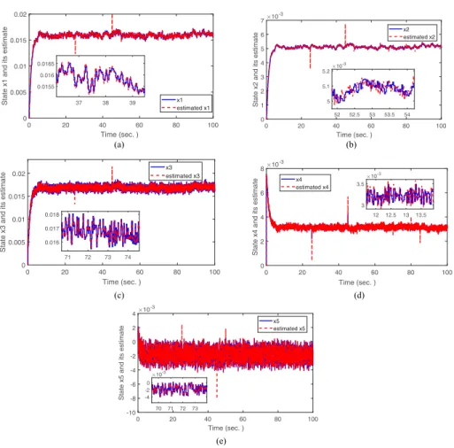
FIGURE 1. (a) System statex1and its estimate. (b) System statex2and its estimate. (c) System statex3 and its estimate. (d) System statex4and its estimate. (e) System statex5and its estimate.
and the sampling period Ts = 0.026 s. The total running
time is 100 seconds. The unknown inputs are given as random signals with range from−10−2to 10−2. Actuator fault vector is fa = fa1 fa2T, where fa1 is 10% loss of actuation
effectiveness from 25 second to 45 second, andfa2is−0.5+
0.1sin(kTs) from 50 second to 65 second. In this case, the
dis-tribution matrix of the actuator fault vector is Bfa = B.
Sensor faultfs =
fs1 fs2Toccurs in the first two outputs,
where fs1 is 15% loss of effectiveness from 70 second to
80 second, and fs2 is a stuck fault from 85 second. Then Dfs=
1 0 0 0 0 0 1 0 0 0
T
. Consequently, the fault vector consid-ered is f = faT fsTT withBf = [Bfa 05×2] andDf =
[ 05×2Dfs].
H can be solved from (13). Selectingγd2 = 0.01,γds =
0.08,γds1 =0.06,andα =0.05, and solving the LMI (18),
the observer gainL1 can be calculated. ThereforeRandL2
can be obtained following the formulae (10) and (12), respec-tively. As a result, the obtained gains of the UIO in the form of (4), that is,H,T,L1,RandL2, are shown in (70) at the top
of the next page.
There is a pre-designed feedback controller
u(k)=Ky(k) (71)
FIGURE 2. Actuator faults and their estimates.
where the control gain is given by [13], as follows
K= −0.0346 0.1076 −0.0120 0.0096 −0.0135 0.0376 −0.1703 0.0139 −0.0111 0.0156 .
In this case, the tolerant controller is in the form of
u(k)=Kyc(k)−KfJ2xˆ¯(k) (72) whereKf = 1 0 0 0 0 1 0 0 , andJ2=04×5I4.
Figures 1(a)-1(e) show five system states and their esti-mates, while Figures 2 and 3 exhibit the faults and their
H = 0.1636 0.1091 −0.0545 0.2727 0.2182 0.1091 0.0727 −0.0364 0.1818 0.1455 −0.0545 −0.0364 0.0182 −0.0909 −0.0727 0.2727 0.1818 −0.0909 0.4545 0.3636 0.2182 0.1455 −0.0727 0.3636 0.2909 0 0 0 0 0 0 0 0 0 0 0 0 0 0 0 0 0 0 0 0 T = 0.8364 −0.1091 0.0545 −0.2727 −0.2182 0 0 −0.1636 −0.1091 −0.1091 0.9273 0.0364 −0.1818 −0.1455 0 0 −0.1091 −0.0727 0.0545 0.0364 0.9818 0.0909 0.0727 0 0 0.0545 0.0364 −0.2727 −0.1818 0.0909 0.5455 −0.3636 0 0 −0.2727 −0.1818 −0.2182 −0.1455 0.0727 −0.3636 0.7091 0 0 −0.2182 −0.1455 0 0 0 0 0 1 0 0 0 0 0 0 0 0 0 1 0 0 0 0 0 0 0 0 0 1 0 0 0 0 0 0 0 0 0 1 L1 = −1.1697 −0.7800 12.119 8.9338 −10.140 −0.5135 0.3424 −5.1466 3.7253 −4.1978 −0.9721 −0.6482 −12.619 9.1329 −10.086 −0.9573 −0.6383 −9.2758 6.5616 −7.4296 1.2829 0.8555 19.7218 −13.563 15.8453 0.7847 0.5270 62.495 −22.365 46.383 20.052 13.3865 1614.5 417.499 −854.99 1.1034 0.0691 0.1857 −0.7713 0.6238 −0.0457 0.9694 0.1857 −0.6803 0.3114 R= −3.2841 21.862 10.354 −7.5231 8.1382 −0.0025 0.0006 1.0061 0.6709 −1.5177 9.2926 4.4470 −3.1708 3.4220 −0.0017 0.0003 0.4045 0.2697 −4.7293 25.048 10.951 −7.8331 8.2596 0.0041 0.0005 1.0266 0.6846 −3.6067 17.5601 7.7338 −5.3394 5.6717 0.0034 0.0004 0.6846 0.4565 7.3527 −36.194 −16.538 11.025 −12.22 −0.0004 −0.0010 −1.5011 −1.001 −0.7847 −0.5270 −62.495 22.365 −46.383 1 0 −0.7847 −0.5270 −20.052 −13.3865 −1614.5 −417.499 854.99 0 1 −20.052 −13.387 −1.1034 −0.0691 −0.1857 0.7713 −0.6238 0 0 −0.1034 −0.0691 0.0457 −0.9694 −0.1857 0.6803 −0.3114 0 0 0.0457 0.0306 L2 = 1.0066 0.6711 −0.3355 1.6777 1.3421 0.4047 0.2698 −0.1349 0.6745 0.5396 1.0270 0.6847 −0.3423 1.7117 1.3694 0.6849 0.4566 −0.2283 1.1415 0.9132 −1.5017 −1.0011 0.5006 −2.5028 −2.0022 −0.7975 −0.5317 0.2658 −1.3292 −1.0633 −20.1260 −13.4173 6.7087 −33.5434 −26.8347 −0.1037 −0.0691 0.0346 −0.1729 −0.1383 0.0456 0.0304 −0.0152 0.0760 0.0608 (70)
estimates. One can see both the system states and the monitored actuator and sensor faults are estimated excel-lently. The influences of the unknown inputs are decou-pled/attenuated successfully.
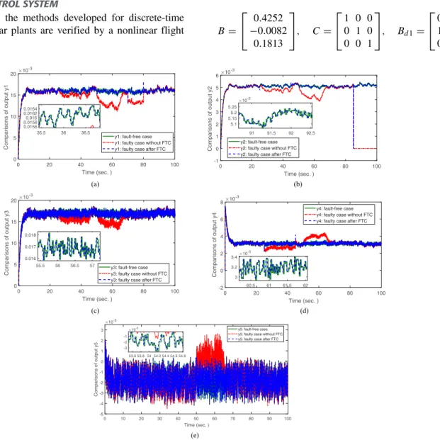
Fig. 4 (a)-(e) exhibit five system outputs under three sce-narios for comparisons: healthy outputs in fault-free cases,
faulty cases without fault tolerant control (FTC), and faulty cases after FTC. From Figure 4, one can see that the faults have made the outputs significantly distorted compared with the healthy system outputs. However, after signal compensa-tion (e.g., FTC), the system outputs are recovered success-fully which are consistent with the healthy system outputs.
FIGURE 3. Sensor faults and their estimates.
As a result, the proposed fault estimation and fault tolerant control techniques are effective.
B. FLIGHT CONTROL SYSTEM
In this example, the methods developed for discrete-time Lipchitz nonlinear plants are verified by a nonlinear flight control system.
The model of a simplified longitudinal flight control system can be described by a discrete-time Lipschitz nonlinear system in the form of (55), where x(k) =
η
y(k)ωz(k)δz(k)Twith initial conditionx0=1 0.5 2T, ηy is the normal velocity, ωz is the pitch rate, and δz is
the pitch angle. u(k) is the elevator control signal, tak-ing value at u(k) = 10. The sampling period isTs =
0.01 s. Lipschitz nonlinear component is8 (x(k) ,u(k)) =
0 0.005 sin(x1(k))0
T
. The system parameters are given as follows [26]: A= 0.9944 −0.1203 −0.4302 0.0017 0.9902 −0.0747 0 0.8187 0 , B= 0.4252 −0.0082 0.1813 , C = 1 0 0 0 1 0 0 0 1 , Bd1= 0 1 0 ,
FIGURE 4. (a) Comparisons of outputy1: fault-free output, output subjected to faults without tolerant control, and output subjected to faults after tolerant control. (b) Comparisons of outputy2: fault-free output, output subjected to faults without tolerant control, and output subjected to faults after tolerant control. (c) Comparisons of outputy3: fault-free output, output subjected to faults without tolerant control, and output subjected to faults after tolerant control. (d) Comparisons of outputy4: fault-free output, output subjected to faults without tolerant control, and output subjected to faults after tolerant control. (e) Comparisons of outputy5: fault-free output,output subjected to faults without tolerant control, and output subjected to faults after tolerant control.
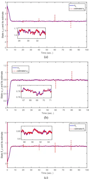
FIGURE 5. (a) Velocityηyand its estimate. (b) Pitch rateωzand its estimate. (c) Pitch angleδzand its estimate.
FIGURE 6. Actuator fault and its estimate.
Bd2 = 0.1 −0.05 0.3 −0.15 −0.4 0.2 , Dd= 0.01 −0.02 0.04 . (73)
The unknown input vectord1(k)=1a21 1a22 1a23x(k)
represents the parameter perturbations in matrix A, i.e.
FIGURE 7. Sensor fault and its estimate.
1a2j=0.1a2j,j=1,2,3. Unknown input vectord2(k)
rep-resents the extra disturbances, with value from−0.01 to 0.01 randomly.ds is the measurement noise vector, taking values
from −0.001 to 0.001. The faults under consideration are 50% loss of the actuation effectivenessfa from 20s to 40s,
and 30% loss of effectivenessfs in the second sensor from
60s to 80s. In this case, Bfa = B, and Dfs = 0 1 0T.
Consequently, the fault vector considered isf = fa fsT
withBf =[Bfa 03×1] andDf =[ 03×1 Dfs].
There is a pre-designed feedback controller
u(k)=Ky(k) (74)
whereK =−
2.1710−9.0038 2.0115
.
Then the fault estimation and fault tolerant control strate-gies designed in Section IV can be implemented to the flight control system.Hcan be solved from (13). Selectingγd2 =
0.05, γds = 0.4, γds1 = 0.03, γθ = 0.05, and α =
0.01, and solving the LMI (60), the observer gainL1can be
calculated. ThereforeRandL2can be obtained following the
formulae (10) and (12), respectively. As a result, the obtained gains of the UIO in the form of (58) are obtained as follows: H = 0 0 0 0 1 0 0 0 0 0 0 0 0 0 0 T = 1 0 0 0 0 0 0 0 0 −1 0 0 1 0 0 0 0 0 1 0 0 0 0 0 1 L1 = 1.8430 −0.0280 −0.4031 −0.3533 0.5063 1.0176 0.0858 1.0168 0.8098 1.9738 0.5029 0.3314 0.3532 −0.5205 −1.0176
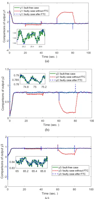
FIGURE 8. (a) Comparison of outputy1: fault-free output,output subjected to faults without tolerant control, and output subjected to faults after tolerant control. (b) Comparison of outputy2: fault-free output,output subjected to faults without tolerant control, and output subjected to faults after tolerant control. (c) Comparison of outputy3: fault-free output,output subjected to faults without tolerant control, and output subjected to faults after tolerant control.
R= −0.8486 −0.0923 −0.0271 0.4252 0.0280 0.3533 −0.5063 −1.0176 0 −1.5063 −0.0858 −0.1981 −0.8098 0.1813 −1.0168 −1.9738 −0.5029 −0.3314 1 −0.5029 −0.3532 0.5205 1.0176 0 1.5205 L2= 0 −0.0923 0 0 −0.5063 0 0 −0.1981 0 0 −0.5029 0 0 0.5205 0 (75)
The tolerant controller should be in the form of
u(k)=Kyc(k)−KfJ2xˆ¯(k) (76)
where Kf = 1 0, J2 = 02×3I2, and K is defined
immediately after (74).
The estimation performances of full system states, i.e. velocity, pitch rate, and pitch angle, are shown in Figures 5(a)-(5c). The actuator and sensor faults and their estimates are depicted by Figures 6 and 7. One can see both the system states and faults are estimated satisfactorily.
The curves displayed in Figures 8(a)-(c) show the com-parisons of the three system outputs under three scenarios: healthy system outputs, faulty system outputs without FTC, and faulty system outputs after FTC. One can see the faulty system output performances are significantly degraded if no measures are taken. However, it is encouraging to see the effects from the faults are successfully mitigated/removed by using the proposed tolerant control strategy. As a result, the developed integrated fault tolerant technique is effective. VI. CONCLUSION
In this study, an integrated fault tolerant control technique has been developed for discrete-time dynamic systems with applications to aero engine system and flight control system. Augmented approach, UIO and LMI have been integrated to construct a simultaneous state/fault estimator with robustness against partially decoupled unknown inputs and measurement noises. Estimator-based signal compensation, associated with a pre-designed controller, has been then developed to attenu-ate the effects of both actuator and sensor faults. As a result, the system outputs after fault tolerant control can track the healthy outputs satisfactorily. The stabilization of the fault-tolerant control system is addressed in the sense of the input-to-state stability. In the future, it is encouraging to develop fault tolerant control mechanisms for aero engineering sys-tems with higher nonlinearities and stochastic dynamics. APPENDIX
PROOF OF LEMMA 1
According to [17] and [27], the sufficient and necessary conditions for the existence of the UIO (4) for the system (3) are:
rank C¯B¯d1=rank(B¯d1) (A1)
(C¯,A¯1) is a detectable pair, where
¯ A1= In¯−HC¯A¯. (A2) It is noticed that ¯ CB¯d1=C Df Bd1 0lf×ld1 =CBd1 (A3) and
rank(B¯d1)=rank(Bd1) (A4)
Therefore one can observe that condition (i) inLemma 1, that is, rank(CBd1)=rank(Bd1), is equivalent to (A1).
If (A1) holds, (A2) is equivalent to that the transmission zeros from the unknown inputs to the measurements must be stable [17], [27], [28],i.e., rank zIn¯− ¯A − ¯Bd1 ¯ C 0 = ¯n+ld1, ∀zwith |z| ≥1 (A5) It is noticed that rank zIn¯− ¯A − ¯Bd1 ¯ C 0 =rank zIn−A −Bf −Bd1 0lf×n zIlf −Ilf 0lf×ld1 C Df 0p×ld1 = rank " A−In Bf Bd1 C Df 0 # , z=1 rank " A−zIn Bd1 C 0 # +lf, z6=1 (A6)
Therefore, it is clear that the conditions (ii) and (iii)
in Lemma 1, is equivalent to the condition (A5), which
is equivalent to the condition (A2). This completes the proof.
REFERENCES
[1] J. Chen and R. J. Patton,Robust Model-Based Fault Diagnosis for Dynamic Systems. Boston, MA, USA: Kluwer Academic, 1999.
[2] M. Blanke, M. Kinnaert, J. Lunze, and M. Staroswiecki,Diagnosis and Fault Tolerant Control. Berlin, Germany: Springer, 2006.
[3] Z. Gao, C. Cecati, and S. Ding, ‘‘A survey of fault diagnosis and fault-tolerant techniques—Part I: Fault diagnosis with model-based and signal-based approaches,’’IEEE Trans. Ind. Electron., vol. 62, no. 6, pp. 3757–3767, Jun. 2015.
[4] Z. Gao, C. Cecati, and S. Ding, ‘‘A survey of fault diagnosis and fault-tolerant techniques—Part II: Fault diagnosis with knowledge-based and hybrid/active approaches,’’IEEE Trans. Ind. Electron., vol. 62, no. 6, pp. 3768–3774, Jun. 2015.
[5] S. Yin, B. Xiao, S. X. Ding, and D. Zhou, ‘‘A review on recent development of spacecraft attitude fault tolerant control system,’’IEEE Trans. Ind. Electron., vol. 63, no. 5, pp. 3311–3320, May 2016.
[6] J. Marzat, H. Piet-Lahanier, F. Damongeot, and E. Walter, ‘‘Model-based fault diagnosis for aerospace systems: A survey,’’Proc. Inst. Mech. Eng., G, J. Aerosp. Eng., vol. 226, no. 10, pp. 1329–1360, 2012.
[7] A. Zhang, C. Lv, Z. Zhang, and Z. She, ‘‘Finite time fault tolerant attitude control-based observer for a rigid satellite subject to thruster faults,’’IEEE Access, vol. 5, pp. 16808–16817, Aug. 2017.
[8] B. Xiao, Q. Hu, Y. Zhang, and X. Huo, ‘‘Fault-tolerant tracking control of spacecraft with attitude-only measurement under actuator failures,’’
J. Guid. Control Dyn., vol. 37, no. 3, pp. 838–849, May 2014.
[9] Z. Gao and S. X. Ding, ‘‘State and disturbance estimator for time-delay systems with application to fault estimation and signal compen-sation,’’IEEE Trans. Signal Process., vol. 55, no. 12, pp. 5541–5551, Dec. 2007.
[10] Z. Gao, T. Breikin, and H. Wang, ‘‘High-gain estimator and fault-tolerant design with application to a gas turbine dynamic system,’’IEEE Trans. Control Syst. Technol., vol. 15, no. 4, pp. 740–753, Jul. 2007.
[11] K. Zhang, B. Jiang, and P. Shi, ‘‘Adjustable parameter-based dis-tributed fault estimation observer design for multiagent systems with directed graphs,’’ IEEE Trans. Cybern., vol. 47, no. 2, pp. 306–314, Feb. 2017.
[12] H. Alwi and C. Edwards, ‘‘Fault detection and fault-tolerant control of a civil aircraft using a sliding-mode-based scheme,’’IEEE Trans. Control Syst. Technol., vol. 16, no. 3, pp. 499–510, May 2008.
[13] Z. Gao, T. Breikin, and H. Wang, ‘‘Discrete-time proportional and integral observer and observer-based controller for systems with both unknown input and output disturbances,’’Optim. Control Appl. Methods, vol. 29, no. 3, pp. 171–189, May 2008.
[14] K. Zhang, B. Jiang, and P. Shi, ‘‘Fault estimation observer design for discrete-time Takagi–Sugeno fuzzy systems based on piecewise Lyapunov functions,’’ IEEE Trans. Fuzzy. Syst., vol. 20, no. 1, pp. 192–200, Feb. 2012.
[15] Z. Gao, ‘‘Estimation and compensation for Lipschitz nonlinear discrete-time systems subjected to unknown measurement delays,’’IEEE Trans. Ind. Electron., vol. 62, no. 9, pp. 5950–5961, Sep. 2015.
[16] D. Wu, W. Liu, J. Song, and Y. She, ‘‘Fault estimation and fault-tolerant control of wind turbines using the SDW-LSI algorithm,’’IEEE Access, vol. 4, pp. 7223–7231, Oct. 2016.
[17] J. Chen, R. J. Patton, and H. Y. Zhang, ‘‘Design of unknown input observers and robust fault detection filters,’’Int. J. Control, vol. 63, no. 1, pp. 85–105, Jan. 1996.
[18] L. Imsland, T. Johansen, H. Grip, and T. Fossen, ‘‘On nonlinear unknown input observers–applied to lateral vehicle velocity estimation on banked roads,’’Int. J. Control, vol. 80, no. 11, pp. 1741–1750, Nov. 2007. [19] O. Hrizi, B. Boussaid, A. Zouinkhi, and M. Abdelkrim, ‘‘Robust unknown
input observer based fast adaptive fault estimation: Application to unicycle robot,’’ in Proc. Int. Conf. Autom., Control Eng. Comput. Sci., Monastir, Tunisia, Mar. 2014, pp. 186–194.
[20] Z. Gao, X. Liu, and Z. Q. Chen, ‘‘Unknown input observer-based robust fault estimation for systems corrupted by partially decoupled distur-bances,’’ IEEE Trans. Ind. Electron., vol. 63, no. 4, pp. 2537–2547, Apr. 2016.
[21] X. Liu, Z. Gao, and Z. Q. Chen, ‘‘Takagi–Sugeno fuzzy model based fault estimation and signal compensation with application to wind Tur-bines,’’ IEEE Trans. Ind. Electron., vol. 64, no. 7, pp. 5678–5689, Jul. 2017.
[22] W. Hahn,Stability of Motion. Berlin, Germany: Springer-Verlag, 1967. [23] Z.-P. Jiang and Y. Wang, ‘‘Input-to-state stability for discrete-time
nonlin-ear systems,’’Automatica, vol. 37, no. 6, pp. 857–869, Jun. 2001. [24] M. Tabatabaeipour, J. Stoustrup, and T. Bak, ‘‘Fault-tolerant control of
discrete-time LPV systems using virtual actuators and sensors,’’ Int. J. Robust Nonlinear Control, vol. 25, no. 5, pp. 707–734, Mar. 2015. [25] M. Lazar and W. Heemels, ‘‘Global input-to-state stability and stabilization
of discrete-time piecewise affine systems,’’Nonlinear Anal., Hybrid Syst., vol. 2, no. 3, pp. 721–734, Aug. 2008.
[26] J. Chen, ‘‘Robust residual generation for model-based fault diagnosis of dynamic systems,’’ Ph.D. dissertation, Dept. Electron., Univ. York, York, U.K. 1995.
[27] S. Chang, W. You, and P. Hsu, ‘‘Design of general structured observers for linear systems with unknown inputs,’’J. Franklin Inst., vol. 334, no. 2, pp. 213–232, Mar. 1997.
[28] S. Sundaram and C. N. Hadjicostis, ‘‘Delayed observers for linear sys-tems with unknown inputs,’’IEEE Trans. Autom. Control, vol. 52, no. 2, pp. 334–339, Feb. 2007.
XIAOXU LIU (S’15) received the B.S. and M.S. degrees from the Department of Math-ematics, Northeastern University, Shenyang, China, in 2012 and 2014, respectively, and the Ph.D. degree from the Department of Mathemat-ics, Physics and Electrical Engineering, Northum-bria University, Newcastle upon Tyne, U.K., in 2018.
Her research interests include robust fault diag-nosis, fault-tolerant control, nonlinear systems, stochastic systems, fuzzy modeling, and wind turbine energy systems.