Spectrum Management using Markov Decision Processes

(1)

Washington University in St. Louis

Washington University Open Scholarship

Engineering and Applied Science Theses &

Dissertations McKelvey School of Engineering

Summer 8-15-2015

Spectrum Management using Markov Decision

Processes

John Leo Meier

Washington University in St. Louis

Follow this and additional works at:https://openscholarship.wustl.edu/eng_etds Part of theEngineering Commons

This Dissertation is brought to you for free and open access by the McKelvey School of Engineering at Washington University Open Scholarship. It has been accepted for inclusion in Engineering and Applied Science Theses & Dissertations by an authorized administrator of Washington University Open

Recommended Citation

Meier, John Leo, "Spectrum Management using Markov Decision Processes" (2015).Engineering and Applied Science Theses & Dissertations. 134.

(2)

WASHINGTON UNIVERSITY IN ST. LOUIS School of Engineering and Applied Science Department of Computer Science and Engineering

Dissertation Examination Committee: Roger Chamberlain, Co-Chair

Christopher Gill, Co-Chair I-Ting Angelina Lee

Paul Min Dave Peters

Spectrum Management using Markov Decision Processes by

John Leo Meier

A dissertation presented to the Graduate School of Arts and Sciences

of Washington University in partial fulfillment of the requirements for the degree

of Doctor of Philosophy

August 2015 Saint Louis, Missouri

(3)

List of Tables

Table 3.1 Value-optimal policy for Pconf = 0.97. . . 28

Table 3.2 Value-optimal policy for Pconf = 0.7. . . 29

Table 3.3 Value optimal policy that results given the following parameters: 4 channels of spectrum, offered load = OL= 0.4 E (erlangs), signal-to-noise ratio =S/N = 1, and SS and OFDM efficiency =γe = 1. . . 38

Table 4.1 Value-optimal policy for a 2-channel spectrum. . . 45

Table 4.3 Value-optimal policy for an 8-channel spectrum. . . 45

Table 4.5 Offered Load of 0.2 Erlangs. . . 47

Table 4.9 Spread Spectrum Efficiency of 70 Percent. . . 50

Table 4.12 Spread Spectrum Efficiency of 99.9 Percent. . . 51

(6)

Table 4.14 Orthogonal Frequency Division Multiplexing Efficiency of 80 Percent. 52

Table 4.15 Orthogonal Frequency Division Multiplexing Efficiency of 90 Percent. 53

Table 4.16 Orthogonal Frequency Division Multiplexing Efficiency of 99.9 Percent. 53

Table 4.17 Signal-To-Noise Ratio of 1. . . 55

Table 4.21 Transposed representation of value-optimal policy from Table 4.4. . . 61

Table 5.1 Evaluation Parameters. . . 73

Table 5.2 Symbol Definitions. . . 73

Table 5.3 Frequency of Imperfect Allocations. . . 86

Table 5.4 Local Optimality. . . 89

Table B.1 Offered Load of 0.2 Erlangs. . . 104

Table B.5 Offered Load of 1 Erlangs. . . 106

(7)

Table C.1 Spread Spectrum Efficiency of 70 Percent. . . 111

Table C.16 Spread Spectrum Efficiency of 99.1 Percent. . . 118

(8)

Table D.1 Orthogonal Frequency Division Multiplexing Efficiency of 70 Percent. 124

Table D.16 Orthogonal Frequency Division Multiplexing Efficiency of 99.1 Percent. 131 Table D.17 Orthogonal Frequency Division Multiplexing Efficiency of 99.2 Percent. 132 Table D.18 Orthogonal Frequency Division Multiplexing Efficiency of 99.3 Percent. 132

(9)

Table D.19 Orthogonal Frequency Division Multiplexing Efficiency of 99.4 Percent. 133 Table D.20 Orthogonal Frequency Division Multiplexing Efficiency of 99.5 Percent. 133 Table D.21 Orthogonal Frequency Division Multiplexing Efficiency of 99.6 Percent. 134 Table D.22 Orthogonal Frequency Division Multiplexing Efficiency of 99.7 Percent. 134 Table D.23 Orthogonal Frequency Division Multiplexing Efficiency of 99.8 Percent. 135 Table D.24 Orthogonal Frequency Division Multiplexing Efficiency of 99.9 Percent. 135

Table E.1 Value-optimal policy, Signal-to-Noise Ratio of 1. . . 138

Table E.13 Value-optimal policy, Signal-to-Noise Ratio of 8, SS modulation effi-cieny of 0.97. . . 144

Table E.14 Value-optimal policy, Signal-to-Noise Ratio of 8, OFDM modulation efficieny of 0.97. . . 144

(10)

List of Figures

Figure 1.1 The (ISM) bands are a small fraction of US spectrum (from [35]). . . 2

Figure 2.1 OFDM spectrum shape. . . 12

Figure 2.2 SS spectrum shape. . . 12

Figure 3.1 RF spectrum physical model, divided into fixed width channels. Indi-vidual transmitters communicate with the centralized spectrum man-ager for permission to transmit (admission) as well as channel assign-ment (allocation). . . 21

Figure 3.2 State transition diagram for basic Bernoulli MDP. . . 24

Figure 3.3 Basic Bernoulli MDP state transition table. . . 26

Figure 3.4 Basic Bernoulli MDP state transition diagram. . . 27

Figure 3.5 Extended Bernoulli MDP state space diagram, supporting message sizes of 1 or 2 channels. . . 31

Figure 3.6 Extended Bernoulli MDP state space diagram, supporting message sizes of of 1, 2, and 4 channel widths. . . 32

Figure 3.7 State space diagram for multiple modulation types. Number of SS transmitters is shown vertically and number of OFDM transmitters is shown horizontally. Self loops represent ‘na’ actions, vertical rising edges represent ‘as’ actions, horizontal edges to the right represent ‘af’ actions, vertical falling edges and horizontal edges to the left represent message departures (all actions have the same effect). . . . 34

(11)

Figure 4.1 Execution time required to compute value-optimal policies vs. state

space size. . . 43

Figure 4.2 Run-time algorithm to approximate value-optimal policies. Lines (1) to (14) correspond to the restricted region of the state space, and lines (15) to (19) correspond to the unrestricted region. . . 60

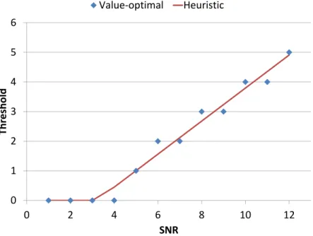
Figure 4.3 Value-optimal and heuristic thresholds separating actions in the re-stricted region in which OFDM modulation is allowed. . . 64

Figure 5.1 Basic Bernoulli MDP state transition diagram. . . 68

Figure 5.2 Pseudo-code of message success or failure. . . 71

Figure 5.3 Example simulator state during a run. . . 72

Figure 5.4 Baseline performance, no overlap (L= 1), no failures (Penv=0.0). . . 76

Figure 5.5 Overlap allowed (L= 3), no failures (Penv=0.0). . . 77

Figure 5.6 No overlap allowed (L= 1), with failures (Penv=0.1). . . 78

Figure 5.7 No overlap allowed (L= 1), with failures (Penv=0.2). . . 79

Figure 5.8 Throughput vs. offered load for both uniform and exponential distribu-tion of message duradistribu-tions, ρ is offered load (λ/µ). Whiskers represent standard deviation. . . 84

Figure 5.9 MDP vs. DES model throughput predictions for Pconf = 0.9, C = 1, L= 1. . . 87

(12)

Acknowledgments

The completion of my Ph.D culminates a life long achievement that has been the most hum-bling accomplishment of my life. The pursuit has enabled me to work with many wonderful and incredibly talented people. I want to thank God for guidance and help. My wife Cindy and children (Elizabeth, Jason, and Jared) made many sacrifices and offered unwavering encouragement enabling me to finish this work. I would like to dedicate this dissertation to my grandchildren (Jaden, Justin, James, and Braden).

My advisors, Roger Chamberlain and Chris Gill, are the most patient, supportive, and giving scientists that I could have hoped to work with. They have been understanding as life events continued to slow my progress over the past several years. I would also like to thank my other committee members, Paul Min, Dave Peters, and Angelina Lee, three professors that have encouraged me as I proposed and defended my dissertation. Thank you.

John Leo Meier

Washington University in Saint Louis August 2015

(13)

ABSTRACT OF THE DISSERTATION

Spectrum Management using Markov Decision Processes by

John Leo Meier

Doctor of Philosophy in Computer Science Washington University in St. Louis, 2015

Professors Roger Chamberlain and Christopher Gill, Co-Chairs

The advent of cognitive radio technology has enabled dramatically more options in the use of RF spectrum, allowing multiple transmitters to effectively share spectrum in ways that were previously unavailable (either due to technical limitations or regulatory restrictions). In this dissertation, we investigate approaches to managing RF spectrum use, with a focus on combining multiple control decisions in a mutually beneficial manner.

Our approach to making spectrum management decisions is grounded in Markov decision theory, which has a rich formal foundation and is frequently used to guide decision making in other disciplines. Here, we develop a set of Markov Decision Processes (MDPs) that model the RF spectrum management problem (in various forms). These MDPs are then queried to provide guidance for management decisions, including the combination of both admission and modulation decisions. This results in control decisions that are optimal in expectation.

To address the computational complexity inherent in computing these control decisions, we develop heuristic approaches that mimic the MDP’s decisions based upon patterns observed in the MDP decision space. These heuristics are shown to closely approximate the optimal results from the the MDP.

(14)

Finally, we empirically assess the appropriateness of using Markov decision theory for RF spectrum management by comparing our MDPs to a discrete-event simulation model that relaxes several of the modeling assumptions made in the development of the MDPs.

(15)

Chapter 1 Introduction

Radio spectrum is a critical scarce resource, commanding billions of dollars [17] for wireless communication companies to enable improved user information transfer. In 1990, there were only 10 million cell phone subscribers worldwide [40], mostly using inefficient analog FM 1G (first generation) cellular RF technology, which provides very low data transfer rates (typically 2.4 kilobits/second) and assigns a channel of spectrum exclusively to each user for the duration of the call. Cell phone usage and user bandwidth demand has grown exponentially, causing new cell phones to rapidly transition to the 4G (fourth generation) standard [34], which uses digital modulation to provide approximately 1 gigabit per second (nearly 1 million times improvement over 1G performance). According to the International Telecommunications Union, the number of active cell phone accounts will soon exceed the world’s population [36].

An important new wireless technology question, then, is how to provide more users with faster service, especially considering the need to improve efficiency in the face of wireless radio interference and other obstacles. A variety of emerging solutions, ranging from cognitive radios for coordinated multi-agency disaster response [49] to industrial process control [46], attempt to answer this question for individual applications. However, an effective spectrum

(16)

allocation method that is able to be customized rigorously across differing features relevant to multiple application domains has not been developed. Furthermore, historically, rigid boundaries tend to divide the available radio frequency (RF) range coarsely into static non-overlapping blocks, each of which accommodates only a very limited number of users.

Figure 1.1: The (ISM) bands are a small fraction of US spectrum (from [35]).

In the United States, the radio spectrum is divided and controlled by the Federal Commu-nications Commission (FCC) and the National Telecommunication and Information Admin-istration (NTIA), which regulate available spectrum. Small sections of unlicensed shared spectrum have promoted the development of more innovative allocation methods.

(17)

To accommodate the rapid increases needed in scalability and data transfer rates, however, there is a need for allocation algorithms that can improve spectrum reuse even further. Stud-ies suggest that RF spectrum can be used more efficiently by ignoring the arbitrary channel boundaries [49]. Our research explores efficient allocation methods that can be applied to a diverse set of applications using traditional and non-traditional spectrum regions, as de-picted in Figure 1.1. Traditional spectrum regions typically support and enforce channel boundaries, which may limit efficiency, while non-traditional spectrum regions, e.g. shared spectrum, eliminate arbitrary spectrum boundaries to improve spectral reuse efficiency. In-teroperability requirements often do not exist between standards regulating the spectrum, which introduces a further challenge to sharing spectrum efficiently. This lack of coordina-tion can cause poor performance of the user devices due to interference in the small available shared unlicensed operational spectrum, as is also illustrated in Figure 1.1.

Numerous methods exist to manage traditional static licensed spectrum (e.g., cellular com-munications and military restricted bands) and unlicensed dynamic spectrum (e.g., ISM band). Regulatory agencies, such as the United States FCC, typically regulate the spectrum using fixed size channels (e.g., AM radio, FM radio, television channels). In traditional spec-trum management, fixed channels use a single modulation technique, but they don’t reuse the channel to transfer information. Enforcing the approved standard ensures consistent operation of wireless devices.

Much of the recent spectrum management innovation so far has centered upon small sections of unlicensed bands, such as those shown in Figure 1.1. Innovative dynamic allocation al-gorithms have the potential to significantly increase spectrum efficiency. Removing artificial channel boundaries can improve efficiency but creates interoperability challenges.

(18)

Implementation and use of more advanced collision detection and avoidance policies are needed to use improve spectrum utilization [50]. Newer modulation types, such as (direct sequence) spread spectrum (SS), simultaneously use wide-band, pseudo-noise (noise-like) signals that are hard to detect, intercept, demodulate or interfere with, when compared with narrow band modulated signals. Narrow band modulation, such as Orthogonal Frequency Division Multiplexing (OFDM), results in a much higher signal level and lower noise level than SS, exhibiting a high SNR. Spread spectrum wideband and OFDM narrowband signals can occupy the same channels, with a low probability of interference, enabling more signals to co-exist simultaneously.

Dynamic spectrum management protocols used in the ISM band, such as Zigbee (802.15.4) and WLAN (802.11), use narrowband and wideband modulated signals to minimize con-flicts between users, as is also illustrated in Figure 1.1. Selecting the correct modulation combinations at the appropriate time is a key challenge for spectrum reuse.

The motivation of this research is to use the available spectrum efficiently, resulting in improved wireless information transfer rate and scalability. The challenge is that there are frequently many design and control decisions to be made that often have interacting impacts on one another, and the current approaches to making informed decisions are primarily ad hoc and empirically based. This dissertation attempts to provide a formal approach to decision making in the space of RF spectrum management, and the formalism that we investigate is the Markov Decision Process (MDP) [39]

Specifically, we develop a series of MDP models, initially based on a simple RF channel model which we call the Bernoulli model, followed up with a different RF channel model which we call the Shannon model (because it is based on Shannon capacity theory [48]). These MDPs are used to guide control decisions in RF spectrum management.

(19)

One benefit of MDP models is that they provide decision guidance that is long-term optimal (in expectation); however, this comes at high computational cost (exponential in the size of the model’s state space). Following the model development, we design heuristics that have

bounded execution time (i.e., O(1)) yet effectively mimic the design guidance provided by

the formal model. These heuristics exploit patterns that regularly occur in the policies that come out of the original models.

In addition, the use of MDP models is validated by comparing with a discrete-event simula-tion model.

1.1 Research Questions

The central question of this dissertation is to assess the viability of using Markov decision theory in the management of radio frequency (RF) spectrum. We investigate that question by addressing the following set of hypotheses.

1. Markov decision process models can be developed for the purpose of RF spectrum management, with specific management decisions guided by the value-optimal policies determined from the MDPs. Specifically, we hypothesize that MDP models can be developed to guide both admission and modulation decisions effectively with respect to relevant throughput measures.

2. It is possible to formulate efficient and effective heuristics that mimic the value-optimal policies of the MDP models we consider. These heuristics are based on the discovery of efficiently computable boundaries between regions that are characterized by a common action.

(20)

3. There is a reasonable correspondence between the Markovian models used and the physical RF spectrum being managed. Here, we specifically hypothesize that:

(a) throughput can be characterized simply by the mean of message durations and is relatively insensitive to their distribution;

(b) even though imperfect channel allocations will occur in any real system, they are infrequent enough that ignoring them does not have a significant impact on an MDP model’s ability to predict throughput accurately; and

(c) value-optimal policy decisions made by the MDP are at least locally optimal as determined by a discrete-event simulation model.

1.2 Contributions and Dissertation Overview

This dissertation provides evidence in support of each of these hypotheses, as follows. The specific contributions (and their locations within the dissertation) are:

• The development of Markov decision process models to guide control decisions in RF

spectrum management.

– The design and evaluation of a basic Bernoulli MDP that guides admission

de-cisions. This includes the specification of the state space, action set, transition system, reward function, and discount factor (Section 3.2) [32].

– Revalidating, using the above MDP, the already known result that narrowband

modulation techniques, such as OFDM, work best when each transmitter uses a unique channel. This revalidation demonstrates that the MDP can be used to confirm previously known results (Section 3.2).

(21)

– The design and evaluation of an extended Bernoulli MDP that supports messages that occupy multiple channels (Section 3.3).

– The development of empirical evidence that greedy allocation algorithms are

suf-ficiently good that ideal allocations can be assumed within these MDP models (Section 5.4) [32].

– The design and evaluation of a Shannon MDP that guides admission and

modu-lation decisions (Section 3.4) [30].

– The execution of a parametric empirical evaluation of the value-optimal policies

that result from the Shannon MDP (Section 4.1) [30].

• The development of efficient heuristics that effectively mimic the value-optimal policies

of the MDPs.

– The discovery of regular patterns in the value-optimal policies of the MDPs. There

are boundaries the separate regions of the state space that have common actions in the value-optimal policies (Sections 3.2 and 4.1) [30].

– The characterization of these patterns in the basic Bernoulli MDP so that

admis-sion deciadmis-sions can be executed via a simple threshold test (Section 3.2) [32].

– The characterization of these patterns in the Shannon MDP so that admission

and modulation decisions can be made in O(1) time (Section 4.2) [30].

• The cross-validation of several models of RF spectrum performance.

– The design and implementation of a discrete-event simulation model of message

(22)

– The development of an M/M/c/c queueing theoretic model and its comparison with the performance predictions of the discrete-event simulation model (Sec-tion 5.3) [31].

– The comparison of the Bernoulli MDP models with the discrete-event simulation

model, both in terms of performance predictions and local optimality of the MDP’s value-optimal policies (Section 5.4) [32].

Chapter 2 discusses related research on RF spectrum and its management, Markov decision processes and their use, and general model validation approaches. Chapter 3 introduces both our Bernoulli and Shannon MDP models, supporting admission (Bernoulli) and admission and modulation (Shannon) decisions. Chapter 4 performs a parametric empirical evalua-tion of the Shannon MDP, illustrates the patterns that exist in the evaluaevalua-tion, and exploits those patterns to construct heuristics that mimic the MDP’s value-optimal policy. Chap-ter 5 assesses the viability of using MDP models generally in RF spectrum management, by comparing properties of the Bernoulli MDP with both a discrete-event simulation and an analytic queueing model. The results are summarized in Chapter 6 with a brief discussion of potential future work.

(23)

Chapter 2 Background and Related Work

2.1 RF Spectrum

RF communications is a rich field with a long history [37, 51, 62]. This dissertation’s focus is on the management of RF spectrum to help ensure its efficient utilization. Specifically, we are interested in maximizing the effective data transmission throughput in a managed region of spectrum.

There are a number of control parameters that have substantial influence on the overall data throughput (i.e., management choices that RF system designers could potentially have at their disposal). These include (but are not limited to) the following:

• admission decisions – should candidate transmitters be allowed to transmit,

• placement decisions – what frequencies should be occupied by a transmission,

• modulation decisions– which modulation technique should be used,

(24)

• coding choices – what channel codes, error codes, etc., should be used,

• spectrum organization – how should the spectrum be divided into channels, and

• message size – how many channels should an individual message occupy.

In this dissertation, we focus on a subset of the above parameter space, concentrating on admission and modulation decisions, with a limited look at placement decisions.

There are, of course, many other factors that also influence the data throughput, which are not under the control of a system designer. These include environmental noise, fading, multipath interference, offered load, etc. This work assumes that the spectrum manager has no control over these factors, but does have knowledge of their extent, which will be quantified using commonly utilized aggregations (articulated in Section 3.1).

While the admissions decision itself is fairly straightforward to understand in simple terms (i.e., when a transmitter wishes to send a message, the management function is to decide whether or not to allow that message to be sent), there has been substantial prior work in how to make this decision effectively. For example, Fu et al. [12] describe a mechanism for re-using channels in a cellular system that allows for greater capacity (i.e., more admissions).

There are a multitude of modulation options available today, including amplitude tion (AM), frequency modulation (FM), phase shift keying (PSK), pulse-position modula-tion (PPM), orthogonal frequency division multiplexing (OFDM), frequency hopping spread spectrum (FH-SS), direct-sequence spread spectrum (DS-SS), and quadrature amplitude modulation (QAM) [62]. We next describe the two modulation options we consider in this work, and defer consideration of others to future work.

(25)

Many RF systems have predefined modulation selected based on the type of service (e.g., video, text, voice), desired quality, available bandwidth, and other factors. Two common modulation types used for voice and data are orthogonal frequency division multiplexing (OFDM) and direct-sequence spread spectrum (SS). OFDM and SS offer two distinctly different modulation types that have different system characteristics, which is helpful to show how such difference may impact modeling and policy generation issues explored in this dissertation.

OFDM modulation is characterized by concentrating the RF signal power within a single channel of some fixed bandwidth. The signal power of a real OFDM transmitter does not evenly fill the channel with power (i.e. a peak signal is located in the center of the channel with exponential decay of the power beyond the channel boundary) as shown in Figure 2.1. OFDM modulators are simpler to construct (relative to SS) but the resulting system has less tolerance of interfering signals. OFDM is relatively robust against multipath fading and inter-symbol interference. In this work, we assume there is perfect channel independence (i.e., we do not model the interference due to imperfect channel separation).

SS modulation distributes the signal power across multiple channels. This implies a pro-portionally lower signal strength in each individual channel. In this work, we will focus exclusively on direct-sequence SS modulation, which uses pseudo-noise codes to phase shift the signal as the spreading mechanism. We make the simplifying assumption that the SS modulation distributes the signal power across the entire region of spectrum being managed, and defer consideration of SS modulation over smaller sub-regions of spectrum to future work. Figure 2.2 illustrates the signal power distribution for a 4 channel example spectrum using SS modulation. Note that the area under the curve (which represents total signal power) is comparable to that of the OFDM example shown in Figure 2.1.

(26)

Figure 2.1: OFDM spectrum shape.

(27)

2.2 Markov Decision Process Models

The following exposition is derived from Tidwell [56], which applies a Markov Decision

Pro-cess (MDP) model to proPro-cessor allocation problems1. The five-tuple (X,A, T, R, γ) describes

a discrete-time MDP. The states are designated as χ ∈ X, and actions are designated as

a ∈ A. The transition system, T, gives the probability PT(χ0 | χ, a) of transitioning from

state χ to state χ0 on action a. The reward function R(χ, a, χ0)∈_R≥0 describes the reward

that accrues when transitioning from stateχto stateχ0 via actiona. The discount factor,γ,

provides a means to ensure the convergence of the long term reward, and is a value greater than 0 but less than or equal to 1, denoted as [0, 1). This discount factor defines how po-tential future rewards are weighed against immediate rewards when evaluating the impact of taking a given action in a given state.

A policy, π, maps states in X to actions in A. At each discrete decision epoch k the agent

observes the state of the MDP χk, then selects an action ak = π(χk). The MDP then

transitions to state χk+1 with probability PT(χk+1 | χk, ak) and yields immediate reward

rk =R(χk, ak, χk+1).

Given discount factor γ, the value of a policy, denoted by Vπ_{, is the expected sum of}

long-term, discounted rewards obtained while following that policy,

Vπ(χ) = E ( _∞ X k=0 γkrk |χ0 =χ, ak =π(χk) ) . (2.1)

1_{Despite the differing resources (RF spectrum vs. processor cycles) and semantic models (allocation vs.}

time-utility scheduling) involved, our formulation of the MDPs in this work is similarly motivated by the challenge of optimal resource use considered in that work.

(28)

Rπ _{denotes the expected reward obtained when executing action} _a₌_π₍_χ_{) in state} _χ_.

Rπ(χ) = X x∈X

PT (x|χ, π(χ))Vπ(x) (2.2)

Then we may equivalently define Vπ _{as the solution to the linear system}

Vπ(χ) =Rπ(χ) +γX x∈X

PT (x|χ, π(χ))Vπ(x) (2.3)

for each state χ. When |Rπ(χ)| is bounded for all states, the discount factor γ prevents

Vπ from diverging for any choice of policy, and can be interpreted as the prior probability

that the system persists from one decision epoch to the next [22]. In practice this value is

almost always set very close to 1 and in this work we set γ to 0.99 (following established

convention [39, 57]).

There are several techniques for computing the value-optimal policy for an MDP with finite

state and action spaces [39]. These techniques calculate the optimal action,π∗(χ), for every

state χ∈ X: π∗(χ) = arg max a∈A ( R(χ, a) +γX x∈X PT (x|χ, a)V∗(x) ) (2.4)

where the optimal value, V∗(χ), is given by:

V∗(χ) = max a∈A ( R(χ, a) +γX x∈X PT (x|χ, a)V∗(x) ) . (2.5)

The value-optimal policy is the policy that optimizes long term value within the MDP, in contrast to immediate reward.

(29)

2.3 Uses of Markov Decision Process Models

Markov decision processes have been used extensively to optimize control of systems [1, 47], particularly those that include stochastic elements [7]. Here, we investigate the viability of using an MDP to optimize decisions in the context of managing RF spectrum. These decisions might be admission decisions, channel allocation decisions, modulation decisions, transmitter power level decisions, or any number of other choices that are germane to man-aging the shared use of the spectrum.

Our work closely follows the approaches of Glaubius et al. [14, 15, 16] and Tidwell et al. [56, 57], which used MDP theory to inform resource scheduling decisions in a real time embedded systems context, where the duration of resource allocations is stochastic. The work of Glaubius focused on proportional sharing of a single discretely time-sliced resource. The work of Tidwell considered arbitrary utility functions in the valuation of individual scheduling decisions. In these works, the authors identified boundaries in the MDP state space that separate the value-optimal actions, which then led to efficient heuristics that closely approximate the value-optimal policies.

Our work follows a similar path, with some important distinctions. First, both Glaubius and Tidwell were working in the domain of real-time scheduling. Our domain is RF spectrum management. By describing a family of MDP models, we demonstrate the applicability of MDP theory over a range of applications in spectrum management. This is further supported by the use of more than one reward function within the family of models we consider.

Second, their initially specified state space was infinite, and (using various techniques that they introduced) they formulated bounded versions that were demonstrably equivalent to the infinite spaces. In our case, the initial state space is constructed in such a way that it

(30)

naturally has bounded extent. This implies that there are edge case considerations in our MDPs that must be explicitly handled, which was not the case in the previous work.

Third, the applicability of the underlying MDP models to the problem domain was not a point of investigation by Glaubius or Tidwell. In our domain, we use a discrete-event simulation model to assess the appropriateness of the family of MDP models to spectrum management.

This dissertation is not the first to suggest using MDPs to guide decision making in RF systems. Zhao et al. [61] propose the use of MDPs for guiding what they call opportunistic spectrum access (the ability of secondary users to identify and exploit instantaneous spectrum use opportunities that arise because of the bursty traffic patterns of primary users). Tradeoffs between optimality and complexity in such cases are examined by Djonin et al. [11]. Akbar and Tranter [2] use hidden Markov models (HMMs) to model and predict the spectrum occupancy of licensed radio bands for this same purpose.

Markovian models have been used to characterize other properties of RF systems as well. Wang et al. [59] use a Markov transition system to characterize different handoff delays associated with connections in cognitive radio networks. Geirhofer et al. [13] propose a continuous-time semi-Markov model of a WLAN’s behavior, towards a better understanding of primary users’ activities.

2.4 Validation of Models

In Chapter 5 we assess the applicability of Markovian models to managing wireless radio spectrum. Perhaps the most relevant results in model applicability come from the domain

(31)

of finite-element modeling [54, 55], where explicit error estimation is used to select between p-methods and h-methods for analysis. In that work, a quantitative estimate of model error is used to assess whether or not a model is appropriate for a given task.

When to use (or not use) a performance model is a subject that is covered in many perfor-mance modeling texts (see [21, 26, 27] for but a few examples). Unfortunately, the methods described in these texts are often quite labor intensive, typically requiring measurement of the system being modeled for empirical validation. Sargent has written extensively on the subject, with a focus on simulation models rather than analytic models, from origins in the 1970s [42] to a recent comprehensive review [43].

The areas of model selection and validation also have been extensively studied. Model se-lection literature is rooted in multiple fields from operations research [60] where the focus is typically on relating a model to a particular physical process, to machine learning litera-ture [10] where the focus is often on selecting the best predictive model.

Krishnamurthy and Chamberlain [25] directly addressed the question of when their proposed models for bounded queueing systems were applicable, by proposing a pair of explicit tests. The first was derived from a slightly relaxed set of assumptions and the second was empir-ically based. If either test failed, the model was considered to be unreliable. Beard and Chamberlain [6] have investigated the use of flow models combined with queueing models to show that while such models can be quite effective at throughput prediction, they are prone to significant error in predicting queue occupancy.

More commonly, assessment is an empirical exercise, in which the model in question (or more precisely, a set of predictions made by the model) is compared either with measurements of the physical system being modeled (e.g., see [6]) or with a (presumably) more robust

(32)

model. For example, a frequent practice is to utilize simulation models to assess analytic models [28], as we do in this work. Such an approach makes the most sense when: (1) the simulation model explicitly incorporates aspects of the physical system being modeled that are either simplified or completely ignored in the analytic model, and (2) when the simulation model (or other reference model) has been independently evaluated, as are both the case in this work. To assess the applicability of Markovian models to the problem of managing RF spectrum, we compare model predictions to a discrete-event simulation.

(33)

Chapter 3 Markov Decision Process Models for

RF Spectrum Management

The central goal of this dissertation is to assess the viability of using Markov decision theory for context aware configuration of parameters affecting radio frequency (RF) spectrum allo-cation, and in doing so to improve throughput across a range of relevant operating conditions. We investigate that goal in this chapter by addressing the following hypothesis.

Markov Decision Process (MDP) models can be developed for the purpose of selecting and evaluating different combinations of factors affecting RF spectrum management, with specific management decisions guided by the value-optimal policies determined from the specific MDP in use. Specifically, we hypothesize that MDP models, whose parameters encode the different factors, can be devel-oped to guide both admission and modulation decisions effectively with respect to relevant throughput measures.

We develop models of radio frequency (RF) spectrum semantics that are intended to capture throughput, environmental interference, channel interference, message duration, and other relevant factors. We start with a description of the RF spectrum system model that we will

use throughout this work. We refer to this as thephysical model; it is intended to capture the

(34)

developed in the dissertation. We then present three distinct MDP models that capture different characteristics of the physical model, handle different sets of input parameters, and have different spectrum management goals.

The MDPs we develop in this dissertation are intended to represent faithfully the semantics of the physical model described next. We investigate this relationship further in Chapter 5, where the basic Bernoulli MDP developed here is cross-validated using a separately developed discrete-event simulation model.

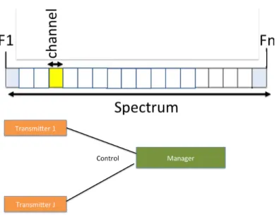
3.1 RF Spectrum Physical Model

In our physical model, the RF medium is a range of radio wave frequencies (e.g., from F1 to Fn), divided into some number of channels (illustrated in Figure 3.1), and a centralized

manager that makes decisions about the use of those channels. With C channels, each

channel has bandwidth (Fn−F1)/C. The channels are rigid, non-overlapping regions of the

RF spectrum for which a centralized manager makes usage decisions.

Messages arrive from transmitters via a Poisson process (utilizing a separatecontrol channel),

are allocated to a channel if admitted, and depart the system if not admitted (i.e., we do not model retries). The manager is responsible for making these admission decisions, which are delivered to the appropriate transmitters (again via a separate control channel that is not explicitly modeled).

We assume the existence of a centralized spectrum resource manager to make decisions that effectively control the use of the media. For example, when the resource manager assigns a

(35)

Figure 3.1: RF spectrum physical model, divided into fixed width channels. Individual transmitters communicate with the centralized spectrum manager for permission to transmit (admission) as well as channel assignment (allocation).

message to a particular channel, the transmitter is then required to transmit exclusively us-ing that sus-ingle channel. For the purposes of this dissertation, we limit such decision-makus-ing to admission, allocation (i.e., selection of a particular channel, including whether or not mes-sages are allowed to overlap), and modulation type. Although the approach developed here could be extended to a de-centralized control scheme, the design issues associated with con-structing such distributed management approaches are beyond the scope of this dissertation. Furthermore, having a centralized resource manager allows it to utilize global information during decision making.

We denote the mean message arrival rate by λ, and message durations are assumed to be

uniformly distributed with mean 1/µ (following the convention in queuing theory that µ is

a service rate). The total rate of departure at any specific time, therefore, is proportional to the number of messages in the system. Multiple messages may be allocated into one channel (i.e., they can overlap); in that case, the probability of successful message delivery

(36)

is a function of the RF channel model, which we describe next. In what follows, we will

use a pair of different channel models, the first referred to as the Bermoulli model and the

second referred to as the Shannon model. Neither is a new proposition, and each has its

foundations in the RF communication literature [37, 51, 62].

The Bernoulli channel model characterizes the probability of success (or failure) of mes-sage delivery in terms of environmental factors and conflicts due to common channel oc-cupancy [19]. Unlike more sophisticated models that attempt to account individually for distinct interference mechanisms [12, 29, 41], the environmental factors (e.g., background

noise, reflections, etc.) are aggregated into a single term, denoted Penv, representing the

probability of a message delivery failure due to these factors. Message conflict is similarly

characterized by a single term, denoted Pconf, which parametrizes a Bernoulli model of

mes-sage failure. The probability that an individual mesmes-sage is successfully delivered, denoted Psucc, is therefore

Psucc = (1−Penv)(1−Pconf)(Nm−1) (3.1)

where Nm is the number of messages sharing the channel.

The Shannon channel model characterizes the throughput achievable on an individual chan-nel via the classic Shannon capacity [48]. Shannon’s Theorem provides a measure of the channel capacity as a function of the available bandwidth and the signal-to-noise ratio

Cs =γeBClog2(1 +S/N), (3.2)

whereCsis the achievable channel capacity (in bits/s),γe is the modulation efficiency,BC is

the channel bandwidth,S is the average signal power (at the receiver), andN is the average

(37)

for an alternate message overlapping in the same spectrum is perceived by the receiver as noise when processing the message of interest.

In both channel models, we assume that transmitters have been sufficiently power-controlled

such that the receiver signal strength is common.2 _{Note that the basic measures provided}

by the Bernoulli model and the Shannon model are different from one another, and thus the reward function of any MDP model based on either a Bernoulli or Shannon channel model will need to account for this distinction.

3.2 Basic MDP Model with a Bernoulli Reward Function

We illustrate the development of MDP models by starting with an initial basic MDP that is designed to make admission decisions based on the Bernoulli channel model. We will refer

to this as the basic Bernoulli MDP model. The goal of the basic Bernoulli MDP model is

to set admission policy, essentially deciding whether an individual channel is to be allocated

(or not allocated) to a newly arriving message (i.e., allowing the transmitter to send the message or not).

This MDP does not make decisions about where to allocate each message. Instead, it assumes the existence of an omniscient (i.e., best possible) allocator that achieves either one channel per message or minimizes message overlap. This is trivially realizable in the circumstances where the number of admitted messages is less than the number of channels available in the spectrum. When the number of messages is greater than the number of channels, we assume that the quantity of messages overlapping one another (i.e., allocated to the same channel)

(38)

Figure 3.2: State transition diagram for basic Bernoulli MDP.

can be minimized. This latter assumption is tested (by comparing with a greedy algorithm) in Chapter 5.

The success or failure of a message delivery is characterized by the Bernoulli channel model,

which incorporates environmental effects (viaPenv) and message conflicts (i.e., message

over-lap, viaPconf). In terms of the effects of such an admission policy, admitting more messages

has the potential to yield higher throughput. However, if the policy admits sufficient mes-sages such that message overlap will occur (i.e., more mesmes-sages are admitted than there are channels available), the channel model reflects this by a diminished probability that either of the messages occupying the same channel will succeed: this in turn diminishes throughput. By designing a reward function that reflects this tradeoff, we can ask the MDP to provide a value-optimal policy that can then be used to make on-line admissions decisions.

3.2.1 States, Actions, and Transitions for the Basic Bernoulli MDP

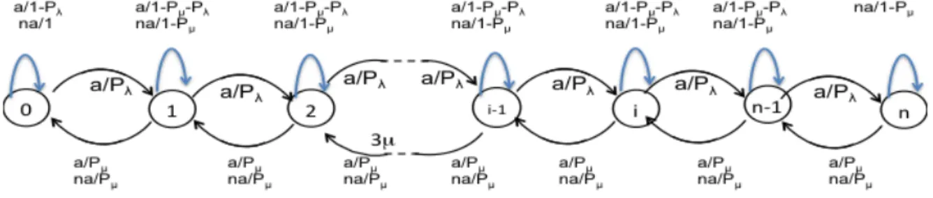
The basic Bernoulli MDP’s state transition system is illustrated in Figure 3.2. Each state

χ=iencodes the number of messages occupying a channel of spectrum (i.e., currently being

transmitted). This MDP model assumes a perfect allocation of messages to channels, so that

if there are C channels and χ ≤ C, each message is assumed to be allocated to a distinct

channel. Ifχ > C, we assume the number of conflicts (i.e., with other messages transmitting

(39)

For admission control, the two possible actions are to accept or not accept. One of these actions is taken whenever a message arrives in the system. In Figure 3.2, actions to accept

are indicated by edges labeled ‘a’ in the transition from a state i to the neighboring state

i+ 1. Similarly, actions to not accept are indicated by edges labeled ‘na’ and are self-loops

(i.e., they transition back into the same state rather than to a new state).

Since the Poisson arrival process has mean rate λ the transition rates for the edges labeled

‘a’ and ‘na’ are both λ. The basic Bernoulli MDP treats the set of messages as a

tradi-tional birth-death process (of the type described by Kleinrock [23]), so the departure rate is

determined by the mean service rate to be χµ.

While this state space could, in principle, be infinite in extent, we artificially bound it to some maximum size under the expectation that above some number of messages it is unreasonable for further admissions to be beneficial in terms of increased throughput.

The above described (continuous-time) model is converted into a discrete-time MDP by adding self-loops and converting the transition rates to transition probabilities using the

uniformization technique described by Grassmann [18] with uniform rate parameterδ which

is set to be greater than the largest rate in the continuous-time model.3 _{As a result, the}

probability of an arrival isλ/δ (for an action to accept) and the probability of a departure is

χµ/δ. The probability of a self-loop is 1−(λ+χµ)/δ (for an action to accept) and 1−χµ/δ

(for an action to not accept). Value (determined according to the reward function described in the next section) is accrued on departure transitions.

After uniformization, the resulting discrete-time MDP is illustrated in Figures 3.3 and 3.4.

The basic Bernoulli MDP is then a four-tuple (X,A, T, R, γ) that consists of a collection of

3_{In the literature the uniform rate parameter is frequently represented by}_γ_{, but we reserve that symbol}

(40)

states X, actions A={a,na}, a transition system T, a reward functionR that specifies the

expected benefit of each action in each state, and a discount factor γ. Figure 3.3 shows the

transition table, wherePλ =λ/δandPµ=χµ/δ. The leftmost column indicates the starting

state and action (one per row), while the remaining columns are marked on the top row by the destination state. The entries in the table represent the probability of transitioning from the starting state to the destination state for each action.

Figure 3.3: Basic Bernoulli MDP state transition table.

Figure 3.4 represents the same information in graphical form, with nodes representing states and action-labeled edges representing transitions. The state diagram provides a visual indi-cation of the transition probability structure of the MDP. In both the state transition table

and diagram, we assume that there is an upper bound of n concurrent messages possible,

and indicate the general interior state with the letter i. Putting these figures into the MDP

notation presented in Chapter 2, for state χ, action aχ =π(χ). The MDP then transitions

(41)

Figure 3.4: Basic Bernoulli MDP state transition diagram.

3.2.2 The Basic Bernoulli Model Reward Function

A policy will be generated by an MDP that maps states in X to actions in A. At each

discrete decision epoch, the policy observes the state of the MDP χ ∈ X, then selects an

action aχ ∈ A. The MDP then transitions to state χ0 with probability PT(χ0|χ, aχ) and the

controller receives reward r=R(χ, aχ, χ0).

The reward function R is defined over the domain of state-action-state tuples, such that

R(χ, a, χ0) is the immediate reward for taking action aχ in state χ and ending up in state

χ0. For the basic Bernoulli MDP, reward is accrued when messages depart the system (i.e.,

transition edges moving from state χ to χ −1). The amount of reward is equal to the

the expected duration of the message time multiplied by the probability that the message

is successfully delivered over the channel, Psucc (see eqn. (3.1)). For all other transitions

(arrivals or self-loops), the reward is zero.

Our approach is based on solving for a policy that is optimal in expectation of accrued long-term reward according to the specified reward function. We used software originally developed by Glaubius et al. [14] to calculate a value-optimal policy for each of the MDPs investigated in the dissertation, by simply via encoding the specifics of the new MDPs in that framework.

(42)

Table 3.1: Value-optimal policy for Pconf = 0.97.

State 0 1 2 3 4 5 6 7 8 9 10 11 12 13 14 15 16

Policy a a a a na na na na na na na na na na na na na

Informally, we expect value-optimal admission decisions made by this MDP to result in an admission policy of accepting incoming messages up to some system occupancy (i.e., number of messages in the system) and then not accepting new messages at any higher

occupancy, with the acceptance threshold being influenced in part by the value of Pconf,

which parametrizes the penalty of sharing individual channels. This policy is frequently used in practice for existing real-world spectrum allocation, e.g., when using FM modulation.

This intuition is confirmed by ramping the value of Pconf down from 1 and looking for

the above pattern when solving for the value-optimal policy using the MDP. In a 4-channel

system (C= 4,n = 16,Penv = 1) the pattern is evident at aPconf of 0.97. This value-optimal

policy is shown in Table 3.1. At this high value of Pconf (i.e., high probability of message

delivery failure due to conflict), sharing of channels is unlikely to benefit throughput, and the policy that is chosen via the MDP is to accept up to 4 messages, but no more. This result is resilient to variation in offered load.

We continue this investigation, ramping down to Pconf = 0.7 in the same 4-channel system

and again solve for the value-optimal policy (shown in Table 3.2). In this case, the resulting policy is to accept up to 8 messages, but no more. This time each channel is potentially shared by up to 2 messages. This pair of experiments helps give us confidence that the MDP is making reasonable admission decisions.

(43)

Table 3.2: Value-optimal policy for Pconf = 0.7.

State 0 1 2 3 4 5 6 7 8 9 10 11 12 13 14 15 16

Policy a a a a a a a a na na na na na na na na na

Given the value-optimal policies generated by the MDP, it is reasonable to consider the development of an on-line run-time admission heuristic that mimics the actions of the value-optimal policy. Such a heuristic can be expressed as follows:

a=      ‘a’ if χ < T h ‘na’ otherwise (3.3)

wherea ∈ Ais the action chosen, χ∈ X is the number of messages currently in the system,

and T h is a fixed threshold. Effectively, the value of the threshold,T h, identifies a decision

boundary, in which the value-optimal action is different above and below the boundary. We

can therefore use the MDP off-line to choose the threshold value, T h, and then use the

heuristic on-line to make the individual admission decisions for each message. Although the

threshold differs between the two experiments (i.e., it is dependent upon the value ofPconf),

its presence in both illustrates the potential for exploiting such decision boundaries, which we develop further in Chapter 4.

In this case, with an appropriate choice of threshold, the on-line heuristic actually mimics the value-optimal policy indicated by the MDP precisely. In Chapter 4, we will return to this approach where an on-line heuristic might not provide a perfect match to the value-optimal policy, but does closely mimic it. In both cases, the on-line decisions take polynomial time, and are therefore considerably more computationally efficient than repeated solving of the MDP for value-optimality.

(44)

3.3 Extending the Basic Bernoulli MDP to Support

Multiple Message Sizes

The basic Bernoulli MDP introduced above is but one example of a whole family of potential MDP models. Here, we extend the basic MDP to support messages that require more than one channel. This is a common technique in RF systems to enable faster delivery of a message, taking advantage of the resulting higher bit rate available when more channels are used [62].

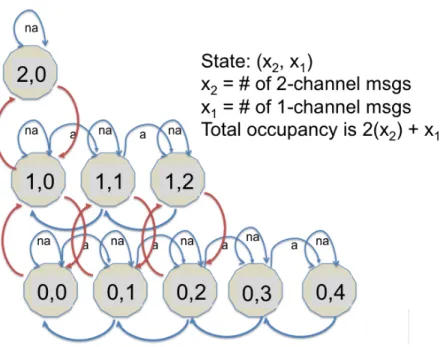
In this extended version of our basic Bernoulli MDP model, we will assume the size of the message (i.e., the number of channels that it occupies) is requested by the transmitter, rather than being decided by the centralized manager. In effect, the manager is still only performing admission decisions. The distinction is that the incoming messages might require more than one channel. Without loss of generality (i.e., by rounding the number of channels needed to the next binary exponent), in the extended MDP model described below the number of channels supported is restricted to be a power of 2.

Figure 3.5 illustrates the state space of an extended Bernoulli MDP model that supports messages of size 1 (i.e., 1 channel) and 2 (i.e., 2 channels). The model encodes the message size in the dimensionality of the state space. Specifically, each state is labeled with an ordered

pair, (x2, x1), where the value of x1 increases horizontally and x2 increases vertically. The

value ofx1 represents the number of messages of size 1 (requiring one channel) and the value

of x2 represents the number of messages of size 2 (requiring 2 channels). For example, the

state (1,1) corresponds to the circumstance where there are 2 messages currently occupying

RF spectrum, with one of the messages consuming one channel and the other message consuming two channels.

(45)

Figure 3.5: Extended Bernoulli MDP state space diagram, supporting message sizes of 1 or 2 channels.

As with the basic Bernoulli MDP, actions are still to accept (‘a’) or to not accept (‘na’), which are shown on the figure only in the horizontal direction. The maximum number of simultaneous messages is bounded by the extent of the MDP state space in each dimension. For the figure, up to 4 single channel messages can be considered and up to 2 dual channel

messages can be considered. Given a total channel count of C, the reward function reflects

the same Bernoulli channel model as above: i.e., allocation is assumed to be ideal (i.e., there are no conflicts) when the number of occupied channels is less than or equal to the number

of channels (2x2+x1 ≤C), and the number of conflicts experienced by any one message is

minimized when 2x2 +x1 > C.

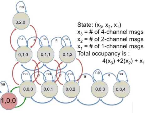
This MDP can be extended to additional dimensions (e.g., 3 dimensions to consider message sizes of 1, 2, and 4) as illustrated in Figure 3.6. In this case, states are labeled via the

(46)

the number of messages using 2 channels, and x3 encodes the number of messages using

4 channels. Actions remain accept (‘a’) and no accept (‘na’). The total number of messages

in the system is indicated by 4x3+ 2x2 +x1. The number of channels is still encoded by

C, and the same Bernoulli reward function is simply extended to the new state encoding

(i.e., reflecting whether or not there is overlap). In this example, the number of channels,C,

is 4 since the state space supports a message that consumes 4 channels, yet the maximum

occupancy for single channel messages is also 4 (i.e.,x1 ≤4).

Figure 3.6: Extended Bernoulli MDP state space diagram, supporting message sizes of of 1, 2, and 4 channel widths.

3.4 Basic MDP Model with a Shannon Reward Function

In this second family of MDP models, we will revert to messages of a common size (one channel), but expand the function of the MDP to include new responsibilities. Here, we will

(47)

ask the MDP to guide the management of both admission decisions and also modulation decisions. The two types of modulation that we will consider are Orthogonal Frequency Division Multiplexing (OFDM), in which each message consumes only a single channel, and Spread Spectrum (SS), in which each message’s transmission is spread across the entire RF spectrum under consideration.

We will also alter the reward function to represent more faithfully the presence of more than one modulation type in common channels of spectrum. This new reward function is based on classic Shannon capacity theory.

3.4.1 States, Actions, and Transitions for the Basic Shannon MDP

The state space diagram for this new MDP is shown in Figure 3.7. States (y2, y1) ∈ X

represent the number of transmitters using each modulation type. Here,y2 is the number of

SS transmitters andy1 is the number of OFDM transmitters. In this case, the actions include

accept SS,‘as’, accept OFDM, ‘af’, and no accept, ‘na’; and therefore A={as,af,na}.

As in the earlier MDP, this continuous-time model is converted to a discrete-time MDP using the uniformization technique described by Grassmann [18]. In the Bernoulli MDPs, value was accrued only on message departure. Here, value is accrued within each state as specified by the Shannon reward function described below.

3.4.2 Shannon Reward Function Design

The reward function for this family of MDPs is based on the Shannon channel model de-scribed in Section 3.1. Given that our high-level goal is to maximize data throughput, we will

(48)

Figure 3.7: State space diagram for multiple modulation types. Number of SS transmitters is shown vertically and number of OFDM transmitters is shown horizontally. Self loops

represent ‘na’ actions, vertical rising edges represent ‘as’ actions, horizontal edges to the

right represent ‘af’ actions, vertical falling edges and horizontal edges to the left represent

message departures (all actions have the same effect).

ask the MDP to optimize a reward function that reflects data throughput. Equation (3.4) below is a restatement of equation (3.2) in Section 3.1.

Cs =γeBClog2(1 +S/N), (3.4)

Recall thatCs is the achievable channel capacity (in bits/s), γe is the modulation efficiency,

BC is the channel bandwidth, S is the average signal power (at the receiver), and N is the

(49)

In what follows, we will explore distinct values of modulation efficiency, γe, for each

mod-ulation type: γe.SS and γe.OF DM. Channel bandwidth, BC, is assumed to be fixed (and

given). Signal power, S, is for a single transmitter that has been admitted to the spectrum

by the central manager. If using OFDM modulation, this signal is limited to a single chan-nel. When using SS modulation, this signal is spread across all channels. We assume that sufficient power control management is in place so that the signal power for each transmitter (for either modulation technique) is the same at the receiver (i.e., transmitters at a farther distance have a greater transmit power). The noise power is a combination of background (environmental) noise and the interference noise generated by other transmitters that are using common spectrum. This implicitly makes the assumptions that (1) OFDM transmit-ters do not share channels, (2) SS transmittransmit-ters all use distinct codes so that they appear as pseudo-random noise to each other and to OFDM transmitters, (3) the interference noise power per transmitter is effectively power controlled in the same way as the intended signal, and (4) noise power is uniformly distributed across each channel.

For each admitted transmitter, equation (3.4) provides the capacity for that individual trans-mitter. The reward is computed as the number of transmitters accepted to transmit using OFDM modulation multiplied by the associated capacity within each channel and the num-ber of spread spectrum transmissions multiplied by their individual capacity. This can be expressed as follows,

R =y2·CSS+y1·COF DM (3.5)

where CSS =Csδ for spread spectrum transmitters, COF DM =Csδ for OFDM transmitters,

andδ is the uniform rate factor, which changes the units of channel capacity,Cs, from bits/s

(50)

We illustrate this reward function via an example, a 2 channel spectrum allocation/modulation problem with a maximum of four transmitters capable of either OFDM or SS modulation.

Here, the signal is assumed to perfectly fill the spectrum (i.e. modulation efficiency, γe, is

assumed to be unity). There are nine total states. We examine each state in turn and

formu-late an expression for the reward. We do this by first articulating values forCSS and COF DM

in terms of the received signal from the transmitter of interest, S, and the environmental

noise, N. When interfering transmitters are included in the expression, the “noise” due to

these transmitters is accounted for by additional instances of S.

The states are configured into a matrix, as shown in Figure 3.8, with the horizontal

di-mension, y1, representing the OFDM modulated signals and the vertical dimension, y2,

representing the SS modulated signals. Starting with state (0,0), we progress horizontally

across the bottom row examining first the OFDM modulated channels (no SS modulation), then vertically up the left-most column allocating SS modulated channels only (no OFDM modulation), and finally examining the remaining states.

State (0,0) indicates all transmitters are off and therefore the reward is zero. Here, both

CSS = 0 andCOF DM = 0.

State (0,1) represents the circumstance where one OFDM transmitter is on. The reward is

given by CSS = 0 and COF DM = BClog2((S/N) + 1) understanding that there is only one

transmitter enabled using OFDM modulation (i.e., one transmitter’s worth of signal,S, only

environmental noise, N, and no interfering transmitters). This is illustrated in Figure 3.8

by the red rectangle in the left channel. The orange rectangle that covers both channels

represents the environmental noise. The overall reward is therefore R = 1 ·COF DM =

(51)

State (0,2) represents the case where two OFDM transmitters are on. The reward is given

byCSS = 0 andCOF DM =BClog2((S/N) + 1), illustrated in the figure by the red and black

rectangles in the two channels. The capacity of each channel is the same as above since they are independent. Since there are two channels in use, the overall reward is therefore R= 2·COF DM = 2BClog2((S/N) + 1). This completes the first row of the state space.

Moving vertically up the initial column, state (1,0) indicates one SS transmitter is sending

signal power S spread over two channels (2BC). The capacity of the spectrum to transmit

the information is given by CSS = 2BClog2((S/2N) + 1), with the environmental noise of 2

channels represented by 2N. This is shown in the figure by the blue rectangle which overs

both channels. Since there are no OFDM transmitters, COF DM = 0. The overall reward is

therefore R= 1·CSS = 2BClog2((S/2N) + 1).

State (2,0) represents a pair of SS transmitters, each spread over the 2 channels of

spec-trum. In this case, each of the transmitters will appear as noise to the other

transmit-ter, contributing an S in the denominator of the Shannon capacity expression. This gives

CSS = 2BClog2

S

2N+S + 1

. Since there are no OFDM transmitters, COF DM = 0, and the

overall reward is therefore R = 2·CSS = 4BClog2

S

2N+S + 1

. This completes the first column of the state space.

Moving to the interior states, state (1,1) indicates two transmitters are on, one using SS

modulation and the other using OFDM modulation. Here, the OFDM transmission

expe-riences both the environmental noise in its assigned channel, N, and one half of the signal

power of the spread spectrum transmitter, 0.5S. This yieldsCOF DM =BClog2 N+0S.5S + 1

. Similarly, the SS transmission experiences both environmental noise (across both channels

Spectrum Management using Markov Decision Processes

Washington University in St. Louis

Washington University Open Scholarship

Spectrum Management using Markov Decision

Processes

John Leo Meier

Table of Contents

List of Tables

List of Figures

Acknowledgments

John Leo Meier

Chapter 1

Introduction

1.1

Research Questions

1.2

Contributions and Dissertation Overview

Chapter 2

Background and Related Work

2.1

RF Spectrum

2.2

Markov Decision Process Models

2.3

Uses of Markov Decision Process Models

2.4

Validation of Models

Chapter 3

Markov Decision Process Models for

RF Spectrum Management

3.1

RF Spectrum Physical Model

3.2

Basic MDP Model with a Bernoulli Reward Function

3.2.1

States, Actions, and Transitions for the Basic Bernoulli MDP

3.2.2

The Basic Bernoulli Model Reward Function

3.3

Extending the Basic Bernoulli MDP to Support

Multiple Message Sizes

3.4

Basic MDP Model with a Shannon Reward Function

3.4.1

States, Actions, and Transitions for the Basic Shannon MDP

3.4.2

Shannon Reward Function Design