Efficient Nonparametric Bayesian Modelling with Sparse
Gaussian Process Approximations
Matthias W. Seeger [email protected]
Max Planck Institute for Biological Cybernetics Spemannstr. 38, T¨ubingen, Germany
Neil D. Lawrence [email protected]
Department of Computer Science, University of Sheffield Regent Court, 211 Portobello St, Sheffield, UK
Ralf Herbrich [email protected]
Microsoft Research Ltd.
7 J J Thomson Ave, Cambridge, UK
Editor: ??
Abstract
Sparse approximations to Bayesian inference for nonparametric Gaussian Process models scale linearly in the number of training points, allowing for the application of powerful kernel-based models to large datasets. We present a general framework based on the informative vector machine (IVM) (Lawrence et al., 2003) and show how the complete Bayesian task of inference and learning of free hyperparameters can be performed in a practically efficient manner. Our framework allows for arbitrary likelihood and kernel functions, so that a large number of elementary models can be treated in a unified way. We present a range of experiments for our method applied to binary classification and regression tasks. Models based on a single latent function can be combined in order to address more complicated setups. We demonstrate this approach for a multi-way classification model.
Keywords: Gaussian Processes, Bayesian Learning, Sparse Approximations, Informative Vector Machine, Hyperparameter Learning, Multi-way Classification, Expectation Propa-gation
1. Introduction
Faced with the task of generalizing from noisy data whose source is imperfectly understood at best,nonparametric smoothingis a powerful and flexible way of analysis and prediction. The idea is to find a function which best satisfies a trade-off between a good data fit
and exhibiting regularity, such as smoothness, periodicity, etc. When compared with the classical parametric approach to statistical modelling, namely to assume simple functional forms such as linearity or low-order polynomials, smoothing is often more flexible and does not suffer from bias which comes from assuming a fixed functional form. A probabilistic Bayesian formulation of smoothing with kernels is achieved by adopting the idea ofGaussian
process(GP) priors (O’Hagan, 1978). By using a Bayesian viewpoint, we obtain a number of
advantages over the traditional setup of finding a penalized best fit. For example, predictive uncertainties can be quantified, and free parameters can be adjusted automatically using
nonlinear optimization. Furthermore, the combination of basic models to address more complicated tasks is straightforward in principle.
A main problem with GP techniques is the unfavourable scaling with the number of datapoints,n, both in terms of computing (typically O(n3)) and of memory usage (O(n2)). Furthermore, even if learning can be accomplished, the final predictor requires at least O(n) time for each prediction, and the whole (training) dataset has to be kept available for prediction. Sparse approximationsto kernel methods (Tipping, 2001, Csat´o and Opper, 2002, Smola and Bartlett, 2001, Williams and Seeger, 2000, Lawrence et al., 2003, Tresp, 2000) are designed to overcome these scaling problems. For somedn, learning with sparse approximations typically scales as O(nd2) time and O(nd) memory, and the prediction cost scales with d only. In this paper we show how a complete Bayesian framework of inference and learning for general models featuring a single latent Gaussian process can be approximated efficiently (i.e. within the sparse constraints just stated). Apart from (Seeger, 2003), we are not aware of prior work on the same scale and generality. Earlier work has either concentrated on the particular GP single regression model with Gaussian noise (Seeger et al., 2003, Snelson and Ghahramani, 2006, Faul and Tipping, 2002), or has not dealt with the important problem of hyperparameter learning within the Bayesian context (Csat´o and Opper, 2002, Lawrence et al., 2003). The framework developed by Seeger (2003) differs from the one presented here, in that a variational approximation to the marginal likelihood is used for hyperparameter learning. We will give some arguments why our criterion here seems preferable. We also give an example of how a number of single process models can be combined into a multi-way classification model in a way that allows the inference techniques to be transferred from the single process case.
The structure of the paper is as follows. In Section 2, we introduce single Gaussian process models together with the main techniques we require in this paper, namely the ex-pectation propagation technique and sparse approximations. In Section 3, we introduce the informative vector machine framework for conditional inference and learning in single GP models. In Section 4, we show how this framework can be used together with multivariate quadrature in order to obtain an IVM solution for multi-way classification. In Section 6, we present a range of experimental results. We close the paper with a discussion in Section 7.
The notation we use in this paper is explained in Appendix A.1.
2. Gaussian Process Models. Sparse Approximations. The Expectation Propagation Algorithm
In this Section, we introduce single Gaussian process models and show how inference and learning can be done in principle. The key problems of non-analytic computations and unfavourable scaling are addressed in turn by introducing sparse approximations and the expectation propagation technique for approximate inference.
2.1 Single Gaussian Process Models
Suppose we are given some dataD={(xi, yi)|i= 1, . . . , n}assumed to be drawn indepen-dently and identically distributed (i.i.d.) from some unknown distribution over X × Y. In order to predict y∗ for further test points x∗, we have to model the regularities that exist in D. In a single GP model, we do this by introducing a latent function u : X → R and
a likelihood distribution P(y|u), y ∈ Y, u ∈ R. We strive for a conditional model which explains the generation of the y = (yi)i given the inputsX ={xi},1 and this is obtained by placing a prior distribution P(u(·)) on the function u. Specifically, we assume thatu(·)
isa prioriaGaussian process(GP) with mean function 0 and covariance functionK(x,x0).
The covariance function is given by
K(x,x0) = E[u(x)u(x0)]
and is positive semidefinite in the sense that for any m∈ Nand ˜x1, . . . ,x˜m we have that the matrix ˜K = (K(˜xi,x˜j))i,j is positive semidefinite,i.e.cTK c˜ ≥0 for allc. Intuitively, the GP is a consistent construction for inducing multivariate Gaussian random variables ˜u
with mean0and covariance matrix ˜K, for any finite set of input points. For more details on GPs for machine learning, the reader may consult (Seeger, 2004, Rasmussen and Williams, 2006).
Let us pause for a moment to see why this setup might achieve our goal of pushing inference from this model to prefer smooth, regular functions over very erratic ones. Many of the most frequently used covariance functions in practice areisotropic, in thatK(x,x0) = K(kx−x0k). Here,K(d) is a nonnegative even function which is monotonically decreasing on [0,∞). The correlation between u(x) andu(x0) is given by K(d)/K(0), d=kx−x0k, which means that as d→ 0, the GP values become perfectly correlated. In mathematical terms, they converge to the same (random) value in mean-square.2 Although the values
u(x) are all random and fluctuate as a whole, they are very strongly correlated at close points, which implies smoothness for functions drawn from the prior. We can also encode other properties of the latent function (which always hold in the mean-square sense) via the choice of the kernel, examples can be found in (Seeger, 2004).
Let u = (u(xi))i ∈ Rn be the variable of u evaluated at the datapoints. Note that
u ∼ P(u) = N(0,K) a priori, where K = (K(xi,xj))i,j is the data covariance (or
ker-nel) matrix. The posterior distribution of u is obtained by Bayes’ formula as P(u|D) ∝ P(y|u)P(u), where P(y|u) = Q
iP(yi|ui), ui = u(xi). Since P(yi|u(·)) = P(yi|ui), the posterior distribution of u(·) is defined throughP(u∗|D) =
R
P(u∗|u)P(u|D)du for points
x∗ and u∗ = u(x∗). This posterior process is not Gaussian in general, but its mean and covariance function can be computed easily once we know mean and covariance matrix of the finite-dimensional posteriorP(u|D). Furthermore, it is usually the case that prior and model come with so-called hyperparameters which have to be adjusted. For example, the likelihood may be a noise distribution whose variance is not known, or the covariance func-tion K has free parameters. An empirical Bayesian method for adjusting such parameters
θ is to consider themarginal likelihood
P(D|θ) =
Z
P(D|u,θ)P(u|θ)du (1) 1. All required input points will always be assumed to be known, and all distributions are always conditioned on all necessary input points. For simplicity, we do not make this explicit in the notation. We also use
Dand the targets interchangeably.
2. One can construct GPs such that the convergence is with probability 1, namely the sample pathu(·) is continuous almost surely.
which serves as a criterion to maximize for selectingθ. Note that again we make use of the fact that the functionu(·) and the datay are independent, conditioned on the valuesu, so that in order to obtainP(D|θ) we only need to integrate over the finite-dimensional u.
In practice, there are at least two problems with this approach. First, the computa-tions of the posteriorP(u|D) and of P(D|θ) are typically analytically intractable. In the special case where the likelihood itself is Gaussian, the posterior and marginal likelihood are Gaussian and can be computed analytically. Much work on GP models for machine learning has concentrated on this case, which however is limited to regression models with Gaussian noise. If P(y|u) is not Gaussian, a general strategy is to approximate P(u|D) by a GaussianQ(u) =Q(u;D). As mentioned above, in order to compute the predictive mean and covariance function of the posterior process u(·)|D(which is not Gaussian in general), all we need are the mean and covariance matrix of P(u|D), so we do not loose anything w.r.t. this task by making a Gaussian approximation. Several concrete methods along this line have been suggested. In this paper we use the expectation propagation(EP) technique (Minka, 2001) in order to compute Q(u) and approximate P(D|θ). This method is intro-duced briefly in Section 2.3. Empirically, the EP technique seems to be more accurate than other variational or saddle-point approximations (Kuss and Rasmussen, 2005).
Second, even ifP(y|u) is Gaussian, the computation ofP(u|D) scales asO(n3) with the numbernof datapoints, which is prohibitive for largen. IfP(u|D) is not tractable, methods for finding an approximate GaussianQ(u) scale asO(n3) as well. Sparse approximations are a general way of overcoming this scaling behaviour at the expense of more approximations. A general framework for sparse approximations has been given by Seeger (2003) and will be reviewed in Section 2.2.
2.2 Sparse Approximations
We are interested in a general way of approximating the posterior computation and repre-sentation and the marginal likelihood computation for the single GP models introduced in Section 2.1. Such a framework has been developed by Seeger (2003), and we will review some aspects here. Recall that P(u|D) ∝ P(D|u)P(u), and the normalization constant is the marginal likelihood. If P(D|u) is not Gaussian, it is approximated by a Gaussian function ofu using a method such as EP (see Section 2.3). For the moment, we assume that P(D|u) is Gaussian. We begin by developing a characterization of sparse GP approxima-tions. Let us define some desirable characteristics of such techniques. First of all, we would like to obtain a predictive approximationP(u∗|D) which is itself a proper Gaussian process. This desideratum already outrules several known methods such as subset of regressors (Sil-verman, 1985) or the relevance vector machine (Tipping, 2001). These have the serious flaw that predictive variance far from the training data is drastically underestimated. In fact, we restrict the procedure to modify the posterior P(uJ|D) on a finite set of input points, the corresponding outputs being denoted byuJ. Exact inference usesuJ =u, the selected input points being the training set, but we allow for other choices. If Q(uJ|D) approxi-matesP(uJ|D), the predictive process must beQ(u∗|D) =
R
P(u∗|uJ)Q(uJ|D)duJ, where P(u∗|uJ) comes from the GP prior. Note thatQ(uJ|D) must be a proper Gaussian. We do not know of any GP method resulting in a proper predictive GP, yet not conforming to this assumption. Next, for each prediction at a test point x∗, we only allow for the evaluation
of O(d) kernel values, namely for K(x∗,x˜i) with dfixed “active” points ˜xi. A few meth-ods have been proposed which do not adhere to this constraint, in that they allow for test points themselves to become active points (Tresp, 2000, Rasmussen and Quinonero Can-dela, 2005). While our reasoning here can be extended to these cases, we do not do so here. In this paper, we will be interested in the case that the active set is part of the training set, which seems reasonable given that the full method is supported on the training points and that observationsyi are available at these points only. However, our reasoning here is not restricted to this case. Denote the active variables by uI = (u(˜xi))i ∈ Rd. One can show (see Appendix A.2) that any sparse approximation conforming to our assumptions can be seen as likelihood approximation: the likelihood functionP(D|u) is effectively replaced by some Gaussian function Q(D|uI) depending on uI only. Note that Q(D|uI) is not a distribution over D, and may be degenerate and unnormalized as Gaussian function. It is important to stress that most such methods donotstrive for a functional approximation of P(D|u) by someQ(D|uI) w.r.t. some norm independent of the GP priorP. As such, the term “likelihood approximation” may be slightly misleading and has lead to suggestions to approximate the prior instead (Quinonero Candela and Rasmussen, 2005). However, the definition in (Seeger, 2003) states that Q(D|uI) should in general be a nonnegative func-tion of some process values uI such that the posterior P(u(·)|D) is approximated well by Q(u(·)|D)∝Q(D|uI)P(u(·)). The term “likelihood approximation” simply means that we get fromP(u(·)|D) toQ(u(·)|D) by formally replacing the likelihood by Q(D|uI).
Suppose now that P(D|u) = NU(u|b,Π), where Π is diagonal. In this paper, the active set is part of the training set, i.e. I ⊂ {1, . . . , n}. How shall we choose Q(D|uI)? The simplest way is to discard the factors corresponding to i6∈I, resulting in Q(D|uI) = NU(uI|bI,ΠI). Note that just as the full likelihoodP(D|u), this approximation factorizes w.r.t. the variablesui, i∈I. Also note that there are only 2dparameters bI,ΠI. Adopting this likelihood approximation leads to the informative vector machine (IVM) (Lawrence et al., 2003, Seeger, 2003). In this paper we restrict ourselves to the IVM approximation, noting that it has clear computational advantages over other non-factorizing approxima-tions, yet is also typically less accurate.
A more accurate likelihood approximation is obtained asQ(D|uI) =NU(EP[u|uI]|b,Π), where EP[u|uI] =K·,IKI−1uI is the conditional mean under the priorP(u). This approxi-mation has been used in (Csat´o and Opper, 2002, Seeger et al., 2003, Seeger, 2003) and can be shown to be optimal w.r.t. some relative entropy argument. Snelson and Ghahramani (2006) note that this likelihood approximation tends to underestimate predictive variance close to the training points. If λ = diag(K −K·,IK−I1KI,·), the likelihood approxima-tion they propose has the form NU(E
P[u|uI]|z,(Π−1+ diagλ)−1) for some z, which (as compared to the previous suggestion) adds some variance except at the active points. This suggestion is optimal under a different relative entropy argument (at least for regression with Gaussian noise). The likelihood approximations of (Seeger et al., 2003, Snelson and Ghahramani, 2006) are more accurate than the factorized one of the IVM, but they also come at significant additional costs. Even in the case of regression with Gaussian noise, at least twice the amount of memory is needed. In case of a non-Gaussian likelihood, it is necessary to estimate the 2nfree parameters of the likelihood approximation, rather than only 2d for the IVM. Strictly speaking, they need to be updated after each inclusion of a pattern intoI. Moreover, if the active setI is determined using greedy forward selection (as
is done for the IVM, see Section 3), it becomes prohibitive to score all remaining points as candidates for each inclusion, while such a complete screening is possible for the IVM. We also cannot afford to compute the same criteria as used with the IVM for many candidates, but have to apply further approximations. Seeger (2003) discusses these issues in detail. We do not consider these more elaborate, costly, and accurate likelihood approximations in this paper, but an extension of our framework to these cases is straightforward in principle and will be addressed in future work.
2.3 Expectation Propagation
The expectation propagation (EP) scheme (Minka, 2001) is a general framework for
ap-proximate inference and learning in probabilistic graphical models. The basic idea and the application to GP models has been suggested already by Opper and Winther (2000) under the name of adaptive TAP approximation. We will only give an intuitive overview here, and refer to (Minka, 2001, Seeger, 2003, 2005) for details.
Suppose we are given the GP model introduced in Section 2.1, with likelihood factors ti(ui) =P(yi|ui) (also called sites here), and recall that we would like to approximate the posteriorP(u|D) and the marginal likelihoodP(D|θ), whereθ collects hyperparameters of the covariance function and the sites. We have already noted that a Gaussian approximation Q(u) ofP(u|D) leads to the fact that the approximate posterior processu(·)|Dis Gaussian, so predictions at test points can be computed easily. EP is a way of obtaining such an approximation, by setting Q(u)∝P(u) n Y i=1 ˜ ti(ui|bi, πi). (2)
Here, ˜ti(ui|bi, πi) = NU(ui|bi, πi) has the form of an (unnormalized) Gaussian (see Ap-pendix A.1), and the site parameters b= (bi)i,Π= diag(πi)i have to be chosen such that Q(u) is a proper Gaussian. EP starts with b = 0,Π =0, i.e. Q= P, then updates the site parameters iteratively. For somei, the intuition behind an EP update is to remove the approximate contribution of i to Q and replace it by the real one, given by the true site ti(ui). The resulting distribution is then projected back to a Gaussian Q0 which is taken to be the new Q. Let Q\i(u) ∝ Q(u)˜ti(ui)−1 be the cavity distribution (where ˜ti(ui) is removed), and define the tilted distribution ˆPi(u)∝ti(ui)Q\i(u). In a sense, ˆPi is a version of Qwhere the approximate effect of iis replaced by the true one. ˆPi is not Gaussian, but the fact that only a single non-Gaussian site is involved, this site depending on a single ui only, allows us to compute mean and covariance of ˆPi. Furthermore, we can choosebi and πi uniquely such that the new Q(u)0 has the same mean and covariance as ˆPi. The latter computation is termed moment matching, another view is that the new Q0 is the closest Gaussian to ˆPi in terms of relative entropy D[ ˆPik ·]. This view and the fact that ˆPi is obtained from the old Qby multiplying with somef(ui) only, implies that the EP update,
i.e.the re-computation ofbi, πi requires knowledge of the current posteriormarginalQ(ui) only. Details about the EP update are given in Appendix B.1. In practice, updates are run until convergence in b,Π. Convergence to some stationary point is not guaranteed in
general, although on GP models with a log-concave likelihood (see Appendix B.1) we have never experienced divergence.3
Note the similarity in form between EP and methods of approximate inference by belief propagation. EP uses current local posterior information in the form of the marginalQ(ui) together with local evidence information in form of the true siteti(ui) in order to update the posterior belief. While the update seems local at first site, in that only the singlebi, πi are updated, it actually has a global reach by affecting all other marginals Q(uj). In sparsely structured graphical networks, these marginals can be updated by message passing along the graph structure. However, if EP is applied to a GP model, the inverse prior covariance matrix K−1 is a dense matrix, so the model cannot be represented by a sparse graph. Updating the marginals Q(uj) after some EP update is a global operation which requires O(n2) in general.
EP comes with an approximation to the marginal likelihood P(D|θ) which works as follows. The approximation ofP(u|D) byQ(u) is done on the basis of matching moments of first and second order between Q and the ˆPi in turn. In order to approximate the nor-malization constant for the posterior, we simply extend this idea to matching the moments of zero order as well. Namely, we use the explicitly normalized site approximationsCit˜i(ui). IfQ\i(ui) is the marginal cavity distribution, we require that the cavity expectation of the true site ti and the site approximation Ci˜ti are the same:
Zi = E\i[ti(ui)] = E\i[Ci˜ti(ui)] =CiZ˜i.
In practice, we run EP updates until the site parameters bi, πi converge, then do a final sweep over all sites in order to compute the Ci factors. We now obtain the approximate marginal likelihood by replacing ti(ui) by Ci˜ti(ui):
Q(D|θ) = exp X i logCi+ Φ[Q]−Φ[P] ! , Φ[N(µ,Σ)] = 1 2log|2πΣ|+ 1 2µ TΣ−1µ. (3)
Note that Φ[P] is the log partition function of the GaussianP when written in exponential family form. In practice, we minimize −logQ(D|θ) w.r.t. θ. Importantly, we can also compute the gradient of this criterion w.r.t.θ. It is shown by Seeger (2005) how this can be done by making use of the fixed point conditions of EP, namely that moments up to second order of ˆPi andQ do match for alli. The validity of these conditions lead to cancellations of terms depending on the mapping of θ to b,Π which in general could not be computed (see Section 3.3 for more on this point).
3. The Informative Vector Machine
In this Section we introduce the informative vector machine (IVM) framework (Lawrence et al., 2003) which combines EM and sparse approximations to achieve efficient inference and learning in single GP models. There are a multitude of such models, including univariate regression (with Gaussian or non-Gaussian noise), binary classification, ordered categorial,
etc.. In fact, any generalized linear model (GLIM) (McCullach and Nelder, 1983) which 3. Divergence in such cases is usually due to numerical instabilities of the updates of theQrepresentation,
comes with a single linear function, gives rise to a single GP model if the linear function is replaced by the latent process. The IVM framework applies to all of these models.
The key features of the IVM as opposed to related approximations is the usage of a factorized likelihood approximation (see Section 2.2), i.e. the simplest and most efficient choice. This fact allows us to devise a particular representation of the posterior belief (the distribution Q(u)) which keeps the full set of marginals Q(uj) up-to-date at any time, at the total cost of only O(nd2). This is important because it allows to use powerful forward selection criteria based on these marginals, thus to screen all remaining points for usefulness as members in I during each inclusion. We do not know of any other sparse approximation framework (apart from the simple, yet often unsatisfactory, heuristic of choosing I completely at random, see Williams and Seeger (2001)) for which this can be done.
3.1 The IVM Representation. Approximate Inference
The Gaussian posterior approximation Q(u) implied by EP has the form (Eq. 2). In the terminology of Section 2.2, NU(u|b,Π) = Qn
i=1˜ti(ui) is a likelihood approximation to
P(D|u). A sparse (efficient) approximation requires that the likelihood approximation is a function ofuIonly, whereI ⊂ {1, . . . , n}is the active set of sized. Within the IVM scheme, this is achieved naturally by simply having bi =πi = 0 for all i6∈I, so the corresponding site approximations ˜ti are constant and drop out. Thus, while a typical application of EP to GP inference requires updates being run until convergence of the site parameters, we restrict ourselves to selecting i ∈I in a data-driven (yet still efficient) manner, and limit EP updates to theseactive i. In this Section, we develop a representation forQ(u) which satisfies the following criteria:
• Upon each inclusion of somej intoI, the representation can be updated in a numeri-cally stable and computationally efficiently manner,i.e.inO(nd) time, requiring the evaluation of a single new column of the kernel matrix K.
• The complete set of marginalsQ(uj), j= 1, . . . , nis a part of the representation. We show how these objectives can be met with a representation of size O(nd). Note that the requirement of having all marginalsQ(uj) accessible at all times is what causes the cost of O(nd) for each inclusion and the dominating size of the representation.4 On the other
hand, we need the marginals in order to perform an informed forward selection ofI, namely so that we can screen all remaining points for each inclusion.
We simplify notation by denoting the currentactivesite parameters byb∈Rd,Π∈Rd,d, whereΠ is diagonal. We also assume that the diagonal entries are nonnegative. In general applications of EP, negativeΠelements are allowed, but may lead to numerical instabilities of the updates. For models we are interested in here, one can show that negative elements cannot occur (see Appendix B.1). The covariance matrixA ofQ(u) is
A = K−1+I·,IΠII,·−1
=K−M MT, M =K·,IΠ1/2L−T,
B =I+Π1/2KIΠ1/2=LLT, (4)
whereL ∈Rd,dis the lower-triangular Cholesky factor of the symmetric positive definiteB. The validity of this representation follows from the Sherman-Morrison-Woodbury formula (Press et al., 1992). Note that this particular form is superior to most other ones suggested in the context of sparse approximations on the basis of numerical stability. B is typically well-conditioned, and the Cholesky decomposition is known to be stable (as opposed to matrix inversions which should be avoided whenever possible).
The stability of EP in the context of the IVM (or full GP inference) hinges on char-acteristics of the likelihood functions ti(ui). We show in Appendix B.1 that IVM updates are numerically stable if the kernel matrix is not poorly conditioned, and the ti(ui) are
log-concave functions of ui, i.e. logti(ui) are concave.5 The latter property is true for
most frequently used likelihoods in Statistics. The most immediate consequence of using a log-concave likelihood together with a Gaussian prior is that the posterior distribution is unimodal. All exponential families (Gaussian, Gamma, Poisson, etc) have log-concave den-sities, the logit and probit classification models are log-concave as well (see Appendix B.1), as are their multivariate variants (see Appendix D). For regression models, very heavy-tailed noise models may fail to be log-concave, examples are the Student-t or the Cauchy distribution. In a sense, the Laplace distributionP(yi|ui)∝exp(−|yi−ui|) is log-concave with the heaviest tails. Since log-concavity implies unimodality, multimodel distributions (such as Gaussian mixtures) are not log-concave either. The IVM framework has been used with multimodal sites (Lawrence and Jordan, 2005), but special care has to be taken to ensure stability.6 We also conjecture (but do not have a proof) that the quality of ap-proximation of the IVM is better for log-concave sites than for others. If the ti are not log-concave, running full EP to convergence might still produce a good approximation, but this is expected to require several iterations over all sites, because the information of some of theti may be contradictory and has to be weighted carefully. For the IVM, we visit each site at most once, and most of the sites are not visited at all. This risky strategy seems somewhat less dangerous in the log-concave case.
The matrix M ∈ Rn,d is called the stub matrix, it dominates the size requirements of the representation, and its update is O(nd). The row MTj,· of M is called stub of j, in that it contains all the information we need to store forj in order to be able to update the marginalQ(uj) efficiently after an inclusion. From (Eq. 4) we see that ifa = diagA, then
a = diagK−diagM MT. Furthermore, the mean h ofQ(u) can be written as
h=M β, β=L−1Π−1/2b.
We see that the maintenance of M in the representation is necessary for being able to updateh,a efficiently, and these are the required parameters of the marginals Q(uj). To conclude, the IVM representation consists of b,π = diagΠ,L,M,β,h,a. The update after an inclusion into I is detailed in Appendix C.1. Note that the dominating cost is 5. It has been observed empirically that log-concavity in the GP model case seems to have other beneficial consequences. For example, EP on the full GP model seems to converge reliably in this case. However, we do not know whether convergence of EP can be guaranteedunder these assumptions.
6. Interestingly, IVM seems to behave more robustly than full EP with sites which are not log-concave. Possible reasons are that IVM does not run EP updates to convergence, but invokes them only once for each active site, and that troublesome patterns (w.r.t. inclusion intoI) are also deemed uninformative by the selection criterion.
a O(nd) matrix-vector multiplication which can be done efficiently by publicly available highly optimized matrix code (such as the ATLAS implementation of BLAS).
In order to predictu∗andy∗for some test pointx∗, we note thatQ(u∗|D) =
R
P(u∗|u)Q(u)du. The predictive distribution is therefore Gaussian,Q(u∗|D) =N(u∗|µ∗, σ2∗), where
µ∗=βTm∗, σ2∗ =K(x∗,x∗)− km∗k2, m∗ =L−1Π1/2(K(xi,x∗))i∈I.
Note that a prediction requires dkernel evaluations only, and the scaling does not depend onn, but only ond. If we only need to evaluateµ∗, we can also precomputep=Π1/2L−Tβ, after which µ∗ can be computed in O(d). We also have Q(y∗|D) = E[P(y∗|u∗)] with the expectation overQ(u∗|D). Desired statistics ofQ(y∗|D) may in general be computed using Gaussian quadrature (see Appendix B.2).
It is important to clarify a point which is frequently misunderstood in the context of IVM. The IVM likelihood approximation does not simply mean that we throw away a large part of the data, namely the points not inI. This would be the case if we did the selection of I without screening all the datapoints, but in case of the IVM we actually spend the dominating effort toscreen all datapoints for every single inclusion, so the selection ofI is very dependent on all data. Readers may recognize a similarity with the support vectors in the support vector machine (SVM) (Sch¨olkopf and Smola, 2002). In both architectures, only a subset of the data has to be available at prediction time, but the subset itself cannot be computed without looking at all the data. A very important difference between IVM and SVM is that for the former, we cancontrolthe degree of sparsity by explicitly choosing d, this not possible for the SVM (the choice of θ has an indirect effect on sparsity in the SVM).
3.2 Greedy Forward Selection. The IVM Algorithm
The IVM representation developed in Section 3.1 keeps all posterior marginals Q(uj) ac-cessible at all times (through h,a). The reason for this is that we intend to use this information in order to screen points j6∈I as candidates for inclusion into I. For example, the marginal variance aj quantifies the remaining uncertainty in the mean prediction hj foruj at pattern xj. Rather than inventing new heuristics, we can tap the field of optimal
design (or active learning), where appropriate criteria for a very related task have been
well-studied. In active learning, we are given a current posterior Q(u) and a pool of candi-date patterns xj without any knowledge of the correspondinguj oryj. We have to select a subset of the patterns which are subsequently labeled (i.e.we obtain the yj), and the goal is to select this set (of a fixed size) in order to gain the most knowledge aboutu(·) from the additional data. In the sequential variant, this subset is of size 1. The sequential approach can always be seen as approximation to the batch variant, in that a subset is selected one pattern at a time. This approximation is called greedy forward selection. Our situation is slightly different and in fact somewhat easier than active learning, in that we can access all yj in the same way as the xj. Typical criteria used in sequential active learning have the form c(xj) = EQ[f(yj, uj,xj)], i.e.the label yj is predicted using the current belief Q(u). If we knowyj (as in our case here), we obtain a stronger variant of the criterion by plugging in the true yj instead of its prediction: ˜c(xj, yj) = EQ[f(yj, uj,xj)], where EQ is over uj only.
Once we have specified a criterion, we select I by successively screening all remaining j and picking the one minimizing the criterion for the next inclusion. We update the IVM representation, and continue untilI has reached the desired maximum size.7 The selection
criterion used by Lawrence et al. (2003) was the differential entropyH[Q0(uj)]−H[Q(uj)], we selected the pattern for which the predictive varianceaj shrinks most with inclusion. In this paper, we focus on theinformation gain score
∆j =−D[Q0(uj)kQ(uj)] =− 1 2 logmj+m−j1+aj−1(h0j −hj)2−1 , mj = 1 +ajπj0, (5) where Q0 is the posterior after inclusion of j into I. Note that this formulation is valid for j 6∈ I, thus bj = πj = 0. As opposed to the differential entropy, ∆j does depend on the posterior mean change as well. For example, in the case of regression with Gaussian noise, the differential entropy score does not even depend on the target yj, and in general the dependence on the actual target is not strong. Note that given hj, aj, computing ∆j requires a single EP update which isO(1) typically, so scoring all remaining patterns isO(n). Note that we can also write ∆j =−D[Q0(u)kQ(u)], becauseQ0(u\j|uj) =Q(u\j|uj) if j is included. The fact that ∆j can be computed based on the marginalQ(uj) only is notan additional approximation.
We can now give a schematic overview of the IVM algorithm for approximate inference (Algorithm 1), given fixed hyperparametersθ. This basic scheme will be embedded below into a procedure for learning θ (Section 3.3), and we give an example of how to use it as subroutine in more complicated models (Section 4).
Algorithm 1 Basic IVM Algorithm
Require: Desired sparsitydn, threshold ε >0 (numerical stability). I =∅,b=0,Π= diag(0),a = diagK, h =0, J ={1, . . . , n}. repeat forj∈J do Compute ∆j (Eq. 5). end for i= argmaxj∈J{∆j|πj0 > ε}
Here,πj0, b0j are computed by an EP update (Appendix B.1). Site updates: πi←π0i, bi ←b0i.
Update representation as shown in Appendix C.1, notablyL,M,a,h. I ←I∪ {i}, J ←J\ {i}.
until |I|=d
It is important to note that rather than running EP on all site parameters until conver-gence, we leave most of the site parameters at 0 (otherwise we would not obtain a sparse IVM approximation), and we update the parameters fori∈I only once, at the time they are included.
7. The maximum size ofI is not a statistical variable, but a parameter of the algorithm. There is no sensible way of selecting an “appropriate size”, since we expect that a larger size works better in general. The size must be chosen based on feasibility considerations.
We finally discuss a simple extension of the basic scheme which is useful if the storage of the completeM is not possible or will lead to performance degradation. In Algorithm 1, the selection setJ of candidates for each inclusion is chosen to be J ={1, . . . , n} \I. We only really needMJ,·, so if we restrictJ to a smaller set, we require less memory and update time. The problem is that it is not efficient to haveJ growat a later stage: the update of
MJ,· when J is extended by j (say) is as expensive as having j in J from the beginning. We use the following strategy which shrinksJ monotonically. We set some upper boundB on the total number ofMJ,·entries, so that|J|d≤B at all times. J remains constant over blocks ofkinclusions.8 At the beginning,J ={1, . . . , n}. After eachkinclusions, we pick a
new sizem0 forJ0. J is first replaced byJ\I. IfJ is still larger thanm0, we keep a certain fraction ρ of entries in J, namely the ones which achieved the best (lowest) scores. The remaining 1−ρ part of J0 is sampled at random from the rest of J. We re-arrange M
J0,·
and continue. This procedure is called randomized greedy selection, a variant was used by Lawrence et al. (2003). The importance of randomized selection is to be able to apply the IVM approximation for active set sizes d even if nd is beyond our memory capacities. In light of the greedy nature of the selection ofI, we expect that the most “important” points are included fairly early, which justifies the successive shrinkage of J during later stages. 3.2.1 Regression with Gaussian Noise
Let us illustrate our general abstract framework for the simple case of univariate regression with Gaussian noise. In this case, P(y|u) = N(y|u, σ2) is already Gaussian, so the EP approximation is not required. We do not have to write special code for this case, however. At the point of inclusion of j (say), we simply set bj = yjσ−2, πj = σ−2. By doing so, we have tj(uj) = ˜tj(uj), i.e.site and site approximation are identical. Therefore, Q(u) is identical to the true posterior P(u|yI). We need to stress again that this does not mean that the IVM blindly throws away much of the data, because the choice ofI depends on all of y. We have that ∆j =− 1 2 logmj+m−j1+ajσ−4m−j2(yj−hj)2−1 , mj = 1 +ajσ−2
for the information gain score. In this example, we can see that the information gain score depends on the predictive mean hj and the true target yj, in that everything else equal, patterns with larger distance |yj −hj| are preferred. This makes sense, as we are looking for patterns which come as “largest surprise” to the current model. As opposed to this, the differential entropy score used by Lawrence et al. (2003) does not depend onyj.
3.3 The Marginal Likelihood Approximation
Recall from Section 2.1 that the marginal likelihood P(D|θ) (Eq. 1) can be used to select appropriate values for the hyperparametersθ which maximizeP(D|θ). This is anempirical
Bayesian procedure. While the correct Bayesian way to deal with θ would be to integrate
them out, in practice the maximization of an approximation of P(D|θ) is often a useful surrogate. Justifications of this procedure can be found in (MacKay, 2003).
8. ChangingJinvolves re-arrangements of the matrix J,·which are themselvesO(nd), so should not be
We noted in Section 2.3 that an approximation to the marginal likelihood can be ob-tained within the EP framework (Eq. 3). Details about this approximate criterion and its gradient are given by Seeger (2005). In this Section, we show how to compute the criterion φ(θ) = −logQ(D|θ) within the IVM framework, and how to obtain an approximation to the gradient ∇ φ. Importantly this is possible within the same O(nd2) time constraint as the inference itself, in fact the latter will still dominate the cost. The details are given in Appendix C.2. φis given in Eq. 11. This criterion is novel to our knowledge. Seeger (2003) considers learningθ for non-regression models, but using a different variational criterion.
In order to efficiently optimize θ, we also need the gradient∇ φ. First of all, the active set I depends on θ, yet this dependence has to be ignored for the gradient computation. However, even for fixed I, the computation of the gradient ∇ φ requires us to know Jaco-bians such as ∇ b,∇ π, and these cannot be computed analytically. Seeger (2005) shows that the problematic terms do actually cancel out if the EP algorithm is applied to full GP inference (without a sparse approximation). The reason is that the following fixed point condition holds for the site parameters once EP converges on them: ˆPi and Q have the same mean and covariance for alli. This is clearly not the case for the IVM approximation, where the site parameters fori6∈I are kept at 0, and even fori∈I we set the parameters only once. Note that for other more expensive sparse approximations, such as the ones mentioned in Section 2.2, the EP fixed point conditions do actually hold (for fixed I), and the exact gradient can be computed. We leave this as a direction for future work, we are not aware of work in that direction for non-Gaussian likelihood (Seeger (2003) computes the exact gradient for a different variational approximation to the marginal likelihood). In the case of IVM, we employ an approximation to the gradient, which is developed in Appendix C.2, and is given in Eq. 14 and Eq. 12.
We note that criterion and gradient computation can be unified with the further ap-proximation of randomized greedy selection (see Section 3.2). Recall that this strategy ends up maintaining only the partMJ,·of the dominating stub matrix, whereJ ⊂ {1, . . . , n} \I is a selection index. Ideally, J contains patterns which carry most additional information, givenQ(u) and the current active setI, and our selection strategy is triggered towards that goal. Therefore, we may replace the parts in the marginal likelihood criterion summing over i6∈I by the corresponding subparts summing over i∈J only. In fact, the derivation of criterion and gradient in Appendix C.2 have been written in terms of J already, so they can be used directly with a selection index.
Our plan is to minimize φw.r.t. θ, using some gradient-based optimizer which employs the conditional inference scheme of Section 3.2 as subroutine. We note that this is not a standard nonlinear optimization problem. First, we can only compute the gradient assuming that the active set I does not depend on the current θ, although strictly speaking it does. The same is true for the selection indexJ if a randomized greedy selection strategy is used (see Section 3.2). Next, even if these dependencies are ignored, we cannot compute the exact gradient∇ φin general, because the EP fixed point conditions do not hold for most patterns i. Still, we observe empirically that the approximate gradient derived in Appendix C.2 is very useful for descending on φ. Our optimization strategy is similar to the one suggested by Seeger (2003). It is iterative, where each iteration step is either major or minor. Each step results in the computation of φ and a ∇ φ approximation, followed by an update of
previous step. The IVM representation of Section 3.1 is computed directly, which scales as O(nd2), but in practice is much faster than doing conditional inference with a re-selection ofI (andJ). We then computeφand the gradient based on the representation. In a major step, we start by calling the conditional inference subroutine of Section 3.2 from scratch, thereby re-selecting I (andJ). We then do the same as during a minor step.
We face an interesting trade-off in the overall optimization. In practice, minor steps are much more efficient than major steps (although both areO(nd2)). Furthermore, doing a major step may introduce discontinuities into the criterion curve φ(θ). On the other hand, running many minor steps in between major ones is risky, because the IVM approx-imation as such, without the forward selection of I, is not a very good approximation to the full posterior, in the sense that the former is more prone to overfitting. Only a fairly frequent reselection of I with points deemed unusual under the current setting ensures a proper weight on complexity control. Our strategy is to use major steps to compute search directions, along which we descend using line searches with minor steps. We can also do major steps only for everyk-th search direction,k >1. With k= 1 and short line searches, we are on the safe side, but such a strategy requires many expensive major mode steps. Some researchers recommended selecting I early and sticking with it, only updating the hyperparameters later on, mainly because this strategy is easier to implement. Based on our experimental experience, we find that this strategy leads to suboptimal results in many cases.
Even within the inner optimization consisting of minor mode steps only, i.e. keeping I fixed, we have several options. Denoting the site parameters by s, we note that φ is really a function φ(θ,s). The gradient given by Eq. 14 and Eq. 12 is ∇ φ(θ,s) for fixed
s, neglecting the fact that s should really depend onθ. Namely, for fixedI we can define
s as mapping of θ through the site updates done in the ordering determined by I. Two strategies for the inner optimization are as follows. We can keep s constant throughout, updating it only together withI in major steps. The advantage is simplicity, since criterion and gradient are compatible and standard code can be used for the inner loops. On the other hand, the wrong criterion is minimized during inner loops. We can also update s
with each criterion evaluation in the inner loops. This requires special “robust” line search code which neglects gradient information, but the correct criterion is minimized (for fixed I). A hybrid is possible as well, in that s is kept constant during line searches, but is recomputed for each new inner loop search direction. It is likely that an optimal strategy depends on the problem at hand and the resources we want to spend, and some fine-tuning is typically required for finding the best option. We present some experiments along these lines in Section 6.1.1.
A final note on the stability and converge properties of this method. Any type of “convergence” to high accuracy cannot be expected, even ifI(andJ) are fixed at some point. In practice, the best we can hope for are final small-scale oscillations around some pointθ. However, at the moment we cannot provide a general convergence proof even guaranteeing such a limit behaviour. Snelson and Ghahramani (2006) propose a sparse approximation for GP regression with Gaussian noise, where the active input points are optimized over together withθ, always converging to a local minimum of their criterion. The advantages and drawbacks of this approach as compared to ours are discussed in Section 7.1.
4. Multi-Way Classification
In Section 3 we developed the IVM representation, conditional inference and learning tech-niques which can be applied to any single GP model. However, a range of important models do not fall into this category, because they require more than a single process to be rep-resented. A natural approach to inference and learning in such a model is to approximate these tasks in a way which allows us to solve them using the single GP IVM framework as principal subroutine. In this Section, rather than trying to formalize another general framework for multi-process models, we concentrate on the concrete example of multi-way
classification. Our approach, however, is general and may apply to other models as well.
For example, it has been used with a multi-output regression model by Teh et al. (2005).
4.1 The Model. Inference Approximation
Suppose now that Y ={1, . . . , C}forC >2. The task therefore is multi-way classification with C classes. A common approach is to allocate a latent variable uc ∈ R for every class, and to define a likelihood P(y|u), u ∈ RC. We will define a concrete classification likelihood below. We now require C latent processes uc(·), which we assume a priori to be independent GPs with covariance functions K(c). A sensible likelihood will couple the
classes, in thatP(y|u) does not factorize as a function of theuc. For such a likelihood, we observe that the posterior processes uc(·) are not independent anymore.
How can we implement sparse inference and learning for the multi-way GP model? A simple idea is to treat the model in the single GP context, by extending x → (x, c), c = 1, . . . , C, with the joint covariance function
K((x, c),(x0, c0)) = I{c=c0}K(c)(x,x0).
The problem with this approach is that forndatapoints and a fixed degree of sparsityd/n, the IVM framework has a complexity ofO(C3nd2), thus scales cubically inC, and we need O(C2nd) memory. Such scaling is prohibitive. In fact, there is a very simple heuristic for dealing with the multi-way problem. Namely, we can learnCpredictors independently, each of which discriminates one of the classes against the union of all others. This one-against-restheuristic scales asO(Cnd2) in the IVM framework. Since it works usually quite well in practice, it seems hard to justify a superlinear scaling in C of a proper multi-way method towards practitioners.
A linear scaling in C can be obtained by making thefactorization assumption that the processes uc(·) are independent under the approximate posteriorQ:
Q(u(·)) = C
Y
c=1
Qc(uc(·)).
Such factorization assumptions are fairly commonly used in variational approximations. While couplings in the true posterior are not represented in the factorizedQ, the parameters of theQc factors are in general influenced by the presence of couplings. Seeger and Jordan (2004b) give a method which represents posterior couplings explicitly, but this is technically much more complicated than the factorized method presented here, and in fact does not lead to an improvement in predictions.
Under this factorization assumption, it becomes clear how the single GP IVM framework can be applied. Namely, eachQc is represented by an IVM representation (see Section 3.1), where we allow for different active sets Ic of potentially different sizes dc. The overall representation size is O(nP
cd2c). Again, we can apply EP (see Section 2.3) in order to deal with the non-Gaussian sites ti(ui) = P(yi|ui), ui ∈ RC. The EP updates work essentially in the same way as before, only that now we haveui∈RC (recall Appendix B.1 for details of the univariate case). Site parameters have the form bi,πi ∈ RC now, and ˜
ti(ui) = NU(bi,diagπi). Note that the site approximations have to be factorized, due to the independence assumptions for the Qc. The cavity distribution Q\i(ui) is factorized as well. For the moment matching, we require expectations of the form
E\ihukcti(ui)
i
, k= 0,1,2. (6)
Note that ti(ui) does not factorize, therefore the tilted distribution ˆPi does not factorize either. However, because we need to retain independence of the Qc, we have to project
ˆ
Pi onto a factorized Gaussian Q0(ui), therefore all we need are means and variances of ˆPi. If we formulate the projection as a relative entropy minimization problem onto factorized Gaussians, we obtain the update formulae
πj,c= (a0j,c−1−a−j,c1)+, bj,c=a−j,c1(h0j,c−hj,c) +πj,ch0j,c, (7) whereh0
j,c, a0j,c are mean and variance of ˆPj(uj,c), and (x)+=xI{x>0}. The quadrature part is challenging in general for all but small C. General rules such as Gaussian quadrature scale exponentially in C (see Appendix B.2). For a particular likelihood and large C, we either need to find a special method of doing the quadratures (we give an example below), or we need to use inaccurate rules together with corrections for the worst artefacts (Lerner (2002) gives an example for the latter).
4.2 The Multivariate Probit Likelihood. Greedy Forward Selection
The outcome of an EP update are new site parameters bi,πi. Based on these, the C independent IVM representations are updated, as is shown in Appendix C.1. We will address the implementation of greedy forward selection of theIc below, but we first need to demonstrate how to compute the quadratures of Eq. 6 efficiently. To this end, we employ a particular likelihood for the multi-way setup: the multivariate probit likelihood. This likelihood is the natural generalization of the probit likelihood (see Appendix B.1) to C classes, namely as Gaussian perturbation of the indicator function of {vy = maxy0vy0}:
P(y|u) = E ∼N(0, ) h I{vy=max y0vy0} i = Eny Y y06=y Eny0 h I{vy≥v y0} i , v =u+p+n. (8)
Here, p ∈ RC are bias parameters which are part of the hyperparameters θ. Expressions of the form of Eq. 6 have the same form as Eq. 8, where v still has a factorized Gaussian distribution (however, with a general diagonal covariance). Furthermore, we see that the coupling between the v components is mediated only through the single component vy.
If we condition on vy, the remaining components can be integrated out independently and analytically, resulting in terms involving the Gaussian c.d.f. Φ(z). Only the final integration over vy has to be done using Gaussian quadrature. Therefore, for any C, the expression of Eq. 6 can be computed in O(C). The details are slightly involved and are given in Appendix D. The usage of the multivariate probit likelihood in the context of sparse GP multi-way classification has been suggested by Seeger and Jordan (2004a) in unpublished work, and independently by Girolami and Rogers (2005).
We note that the multivariate probit likelihood is a log-concave function (this fact is shown in Appendix D). As discussed in Section 3.1, this has important consequences for the numerical stability of EP.
We now show how to generalize the greedy forward selection strategy of Section 3.2, thereby obtaining a conditional inference scheme similar to Algorithm 1, but for the multi-way model. We can score the candidatej for inclusion into Ic by
∆i,c=−D[Q0(uj,c)kQ(uj,c)] =− 1 2 logmj,c+m−j,c1+aj,c−1(h0j,c−hj,c)2−1 , mj,c= 1 +aj,cπ0j,c= max{aj,c/a0j,c,1}.
In practice, the cost of computing a single h0j,c, a0j,c is the same as computing all of h0j,a0j, therefore it makes sense to use a common selection indexJ ⊂ {1, . . . , n}. For each inclusion, we compute the scores ∆j,c for allc, j∈J\Ic, then choose the top-scorer (j, c) for inclusion (namely j into Ic). This selection strategy is combined with randomization in order to shrinkJ during later inclusions. For this shrinkage, the entriesj ofJ are ordered according to minc{∆j,c|j 6∈ Ic}. Note that this means that J may (and should!) include such j for which j ∈Ic already for some c. Empirically, we observe that during early inclusions, we typically see that j is included into Iyj, however during later stages the same j may be
included into other Ic as well. Thus, while clearly (xj, yj) is usually most informative for uyj(·), other types of “informativeness” are considered as well.
We have completed the description of a factorized approximation for sparse conditional inference in the multi-way GP model. The essential steps in this method are calls to the IVM single process subroutines, as well as Gaussian quadratures. The factorization assumption relates our approach to variational mean field approximations, although the latter differ from our method in that the approximationQ minimizes a very different criterion.
5. Further Extensions
In Section 4, we gave a concrete example of how to design a multi-process method based on using the single-process IVM subroutines as major building blocks. In this Section, we provide further examples of how the basic IVM technology has been used to deal with more advanced situations.
Teh et al. (2005) are interested in a model for multi-output regression, where conditional dependencies between the outputs are represented by a linear mixture of latent Gaussian processes, akin to a supervised nonparametric variant of factor analysis. Their model is called semiparametric latent factor model (SLFM). In order to do inference efficiently in SLFMs, one can use a sequence of IVM representations to drive a nonparametric variant of the well-known belief propagation algorithm (Seeger et al., 2004, Seeger, 2006). This
marriage of structured graphical models inference with nonparametric Gaussian fields may have a range of other applications.
Both Seeger and Jordan (2004b) and Girolami and Rogers (2005) employ IVM represen-tations in order to obtain multi-class methods. However, there have been many proposals to approach the multi-class problem using heuristic combinations of binary discriminants, c-against-rest being one of the simpler ones, and some of them perform quite well in prac-tice. Any joint multi-class method has to compete in terms of running time and memory efficiency with these heuristics in order to become interesting to practitioners. Our simple factorizing method of Section 4 does so, while the methods of Seeger and Jordan (2004b), Girolami and Rogers (2005) are more complicated and expensive.
Lawrence and Platt (2004) use the IVM for multi-task learning (aka. hierarchical Bayesian learning). Lawrence and Jordan (2005) employ the IVM for semi-supervised learning, where unlabeled data is used to improve binary classification. The idea is to separate the real line (where the latentu(·) lives) in three categories, rather than two (positive, negative) as used with ordinary classification. The additional “null category” is centered at 0, and unlabeled dataxi is forced not to have their latent value ui in this zone.
Lawrence et al. (2005) try to incorporate invariances w.r.t. transformations ofx into a classifier by adopting the idea of virtual support vectors (see (Sch¨olkopf and Smola, 2002), Sect. 11.3) to the IVM. For example in image classification, a bitmap can be rotated or translated to a certain extent without changing its class membership. The brute force approach to handling such invariances is simply to augment the original data set with virtual points generated by applying small-scale transformations to the data. It is more economical to apply the augmentation to the active points only (the “informative vectors”). In classification, points that are not active often lie far from the decision boundary, so the fitted method is invariant to small-scale transformations of them anyway. Some preliminary experimental results with virtual informative vectors are shown in Section 6.5.
6. Experiments
In this Section, we provide some experimental validation of our framework. These extend the studies which have already been obtained with the IVM in prior work (Lawrence et al., 2003, Seeger, 2003, Teh et al., 2005, Lawrence and Jordan, 2005). Since our framework is very general, we cannot hope to cover its potential applications in much depth here. The code we used for our experiments will be made publicly available for research purposes in the near future, and we hope to stimulate new applications beyond what we suggest in this paper.
6.1 Binary Classification (USPS)
In this Section, we present results on the USPS handwritten digits database (LeCun et al., 1989). The setup closely parallels the study in (Seeger, 2003), Sect. 4.8.4. USPS input points are gray-scale patterns of size 16×16, depicting the digits 0, . . . ,9. The training set contains n= 7291, the test setm= 2007 patterns. We use the correspondingc-against-rest
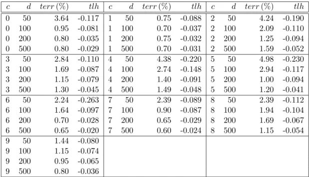
c d terr(%) tlh c d terr(%) tlh c d terr(%) tlh 0 50 3.64 -0.117 1 50 0.75 -0.088 2 50 4.24 -0.190 0 100 0.95 -0.081 1 100 0.70 -0.037 2 100 2.09 -0.110 0 200 0.80 -0.035 1 200 0.75 -0.032 2 200 1.25 -0.094 0 500 0.80 -0.029 1 500 0.70 -0.031 2 500 1.59 -0.052 3 50 2.84 -0.110 4 50 4.38 -0.220 5 50 4.98 -0.230 3 100 1.69 -0.087 4 100 2.74 -0.148 5 100 2.94 -0.117 3 200 1.15 -0.079 4 200 1.40 -0.091 5 200 1.00 -0.094 3 500 1.30 -0.045 4 500 1.49 -0.048 5 500 1.20 -0.041 6 50 2.24 -0.263 7 50 2.39 -0.089 8 50 2.39 -0.112 6 100 1.64 -0.097 7 100 0.90 -0.087 8 100 1.94 -0.104 6 200 0.70 -0.028 7 200 0.65 -0.029 8 200 1.69 -0.067 6 500 0.65 -0.020 7 500 0.60 -0.024 8 500 1.15 -0.054 9 50 1.44 -0.080 9 100 1.15 -0.074 9 200 0.95 -0.065 9 500 0.80 -0.036
Table 1: Results c-against-rest for USPS. d: final active set size. terr: test set error (in percent). tlh: test set average log likelihood.
tasks,c= 0, . . . ,9. We employ theGaussiankernel (also called RBF kernel) K(x,x0) =vexp −w 2pkx−x 0k2 , v, w >0, x∈Rp. (9) We use a hyperpriorP(θ), adding−logP(θ) to the learning criterion. logvisN(−1,1),w−1
is Gamma with mean 1 and degrees of freedom 1. The likelihood is probit classification (see Appendix B.1), with hyperpriorN(0,25) on the intercept parameterβ. The optimization is started fromv= 10, w= 0.0166, the latter being one over the average component variance. We do not employ randomized greedy selection, and we compare different final active set sizes d = 50,100,200,500. For hyperparameter learning, we use the constant strategy described at the end of Section 3.3: the active set I and site parameters are reselected in major steps (outer iterations), but kept constant during the inner iterations (minor steps) (see Section 6.1.1). We allow for 15 outer iterations with a maximum of 8 inner iterations each.9 Results are shown in Table 1.
These results are comparable to the ones obtained in (Seeger, 2003), Sect. 4.8.4, and they are state-of-the-art (see Sch¨olkopf and Smola (2002), Chap. A.1). Note that the test set average log likelihood m−1P
ilogQ(y∗,i|x∗,i, D) always improves with growing active set size, while the test error not always does (the differences in test error between d= 200 and d= 500 are not significant).
9. Judging from plotting the criterion curves, this setting is very conservative, and time can be saved by stopping earlier.
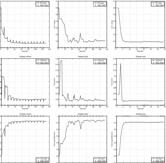
6.1.1 Inner Loop Optimization Strategies
Recall from the end of Section 3.3 that the learning criterion φ is really a function of the hyperparametersθ and the site parameters s, if the latter cannot be considered fixed due to a Gaussian likelihood, and that∇ φis correct only if sis kept fixed. Possible strategies for running the inner optimizations (for fixed active setI) have been stated in Section 3.3, we call them constant (keep s constant during inner loop), hybrid, and exact (updating s
for each criterion evaluation). In this Section, we present a simple comparison for these strategies on the USPS “2”-against-rest task and final active set size d= 200. To this end, we allow for 15 outer iterations of up to 8 inner steps, and protocol the learning criterion together with the test set error and average test set log likelihood. The results are shown in Figure 1.
The final test error and test average log likelihood (after a final major step) are: 0.013453;−0.099876 (constant), 0.016442;−0.064983 (hybrid), 0.014948;−0.091401 (exact). Note that the exact strategy is hampered by our inability of optimizing the criterion appro-priately based on the incorrect gradient, in that more than half of the inner loops terminate with a failed line search. It cannot be recommended together with our present gradient-based optimization. Note also that the criterion curve (upper row) for the constant strategy is comparable to the others only at major steps, since between thesesis kept constant and not reselected. There is an interesting antithetic behaviour between test error and test set log likelihood for the constant strategy: both increase during inner iterations and are decreased by major steps. This supports our hypothesis of a “runaway” effect during in-ner loops. However, the exploration leads to an overall trend of improvement. The hybrid strategy shows some failure patterns, in that the criterion increases during inner loops. This is because the line search optimizes φ(·,s) for fixed s, which is decreased properly indeed, but the subsequent update of s leads to an overall increase. Based on the results here, we favour the constant strategy over the hybrid one, since it is simpler to implement and behaves monotonically decreasing at least during inner iterations.
6.2 Binary Classification (MNIST)
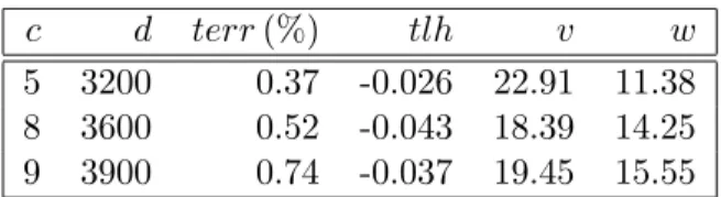
In this Section, we present results on the MNIST handwritten digits database (available at http://www.research.att.com/∼yann/exdb/mnist/index.html). This task has pre-viously been used with IVM in (Lawrence et al., 2003, Seeger, 2003). MNIST input points are gray-scale patterns of size 28×28 which are sparse in that a significant fraction of pixels has value 0. The training set contains n= 60000, the test set m= 10000 patterns. We use the correspondingc-against-rest tasks, restricting our attention to the hardest ones c = 5,8,9. We employ the Gaussian kernel (Eq. 9) with the same hyperprior as in Sec-tion 6.1, starting the optimizaSec-tions from v = 10, w = 0.066. We use final active set sizes d= 3200 (c= 5), d= 3600 (c= 8), and d= 3900 (c = 9). Since the task is much larger than USPS, and the active set sizes are large, we employ randomized greedy selection (see Section 3.2), limitingMJ,˜· to 3.6·107 entries. This means that for the first 100 inclusions,
all remaining patterns are scored. After that, ˜J is shrunk subsequently. The final size of ˜J is 36000000/d, which is 9230 for c= 9. We allow for 7 outer iterations (major steps), each consisting of 4 line searches. The results are shown in Table 2.
0 20 40 60 80 100 120 140 0 0.1 0.2 0.3 0.4 0.5 0.6 0.7 Inner Iter. Crit. Value Strategy constant Phi value Major steps 0 20 40 60 80 100 120 140 0 0.1 0.2 0.3 0.4 0.5 0.6 0.7 Inner Iter. Crit. Value Strategy hybrid Phi value Major steps 0 5 10 15 20 25 30 35 0 0.1 0.2 0.3 0.4 0.5 0.6 0.7 Inner Iter. Crit. Value Strategy exact Phi value Major steps 0 20 40 60 80 100 120 140 0 0.02 0.04 0.06 0.08 0.1 0.12 0.14 0.16 Inner Iter. Test error Strategy constant Test error Major steps 0 20 40 60 80 100 120 140 0 0.02 0.04 0.06 0.08 0.1 0.12 0.14 0.16 Inner Iter. Test error Strategy hybrid Test error Major steps 0 5 10 15 20 25 30 35 0 0.02 0.04 0.06 0.08 0.1 0.12 0.14 0.16 Inner Iter. Test error Strategy exact Test error Major steps 0 20 40 60 80 100 120 140 −0.7 −0.6 −0.5 −0.4 −0.3 −0.2 −0.1 0 Inner Iter.
Test log likelihood
Strategy constant Test log lh Major steps 0 20 40 60 80 100 120 140 −0.7 −0.6 −0.5 −0.4 −0.3 −0.2 −0.1 0 Inner Iter.
Test log likelihood
Strategy hybrid Test log lh Major steps 0 5 10 15 20 25 30 35 −0.7 −0.6 −0.5 −0.4 −0.3 −0.2 −0.1 0 Inner Iter.
Test log likelihood
Strategy exact
Test log lh Major steps
Figure 1: Comparison of inner optimization strategies constant(left column),hybrid (mid-dle column), exact (right column). Criterion value (upper row), test set error (middle row), test set average log likelihood (bottom row).
The results are slightly worse than those quoted in (Lawrence et al., 2003, Seeger, 2003), which can be attributed to the hyperparameter learning procedure behaving suboptimally here. For the experiments in (Lawrence et al., 2003, Seeger, 2003), hyperparameters were selected by validation on a holdout dataset.
c d terr(%) tlh v w 5 3200 0.37 -0.026 22.91 11.38 8 3600 0.52 -0.043 18.39 14.25 9 3900 0.74 -0.037 19.45 15.55
Table 2: Results c-against-rest for MNIST. d: final active set size. terr: test set error (in percent). tlh: test set average log likelihood. v, w: final kernel parameter values.
6.3 Regression with Gaussian Noise (pumadyn-32nm)
In this Section, we present results on the pumadyn-32nm univariate regression dataset contained in the DELVE archive (see www.cs.toronto/∼delve). This set, created using a robot arm simulator, is highly nonlinear and has fairly low noise. There are 32 real-valued attributes, and the database has 8192 cases. We fit a linear discriminant by least squares and subtract this effect off, normalizing the residuals to unit variance. We also normalize each input attribute to unit variance. We then use 10 random splits into training (n= 7192) and test set (m= 1024). Preprocessing and splits are the same as in the studies of Seeger et al. (2003), Seeger (2003). We use thesquared-exponential kernelhere, which is an anisotropic variant of the Gaussian:
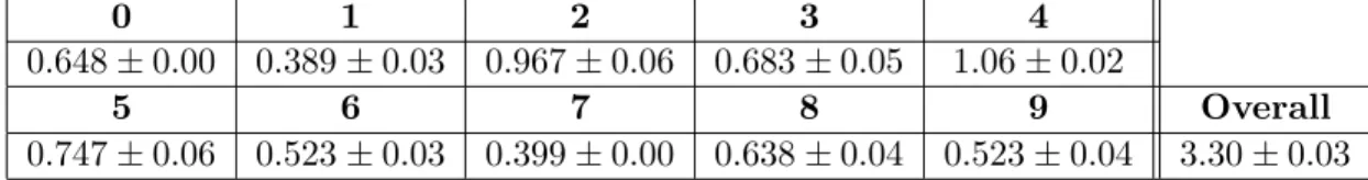
K(x,x0) =vexp −1 2(x−x 0)T(diagw)(x−x0) , v, wj >0, x∈Rp. (10) As opposed to the Gaussian kernel, we have a separate inverse squared length scale pa-rameterwj for each dimension. Importantly, this parameterization implements a technique calledautomatic relevance determination (ARD) (Neal, 1996). Suppose variations in some of the attributesxj are not relevant for explaining the variations in the response y. In this case, the “Occam’s razor” effect embodied in Bayesian estimation techniques will lead to the corresponding wj hyperparameters being driven close to 0. It is important to under-stand that ARD is about conditional variance (or dependence) rather than marginal one. All attributes in our dataset have marginal variance 1, yet only the attributes 5,4,16,15 are significantly relevant for predictingy, all others do not contain useful information. Due to our preprocessing, a linear least squares fit to the data results in a prediction which is constant 0 with mean square (MS) error about 1. If a method fails to identify the relevant attributes, it will in general not perform much better, even if it can represent nonlinear functions. For example, our own method fails if the Gaussian kernel is used, as do related techniques such as SVM regression. Note that in order to implement ARD on this task, we need to learn 34 hyperparameters: the wj, the variancev, and the noise varianceσ2.
Our performance criterion here is average test mean square (MS) error. When comparing our figures here with the results of Seeger et al. (2003), Seeger (2003), note that the latter actually measure 1/2 MS error. Also note that MS error does not depend on the estimates of the predictive variance. Due to the special nature of the task, we can expect two different outcomes in principle. Either, the learning procedure fails to identify and suppress the irrelevant attributes and attains MS error close to 1, or learning succeeds with a MS error